Lecture 6 - University of California, San Diego

Lecture 6

FourierSeriesBasis

GeneralOrthogo-nalExpansions

TheNyquist-ShannonSeriesBasis

TheSamplingTheoremas an Or-thogonalExpansion

RaisedCosineSpectraNyquistPulses

Lecture 6ECE 278 Mathematics for MS Comp Exam

ECE 278 Math for MS Exam- Winter 2019 Lecture 5 1

Lecture 6

FourierSeriesBasis





Fourier Series as a Basis in Signal Space

The set of all complex exponentials ei2πft whose frequency f is an integermultiple of 1/T is a basis {ψn(t)} for signal space on the interval [0,T ].

A function in this signal space can be expanded in a Fourier series using theFourier basis {ψn(t)} = {ein2πft}.

The Fourier coefficients sn are the expansion coefficients in the Fourier basis.

The expansion of an arbitrary function s(t) on the interval [0,T ] is then

s(t) = =

∞∑n=−∞

snψn(t) (1)

=

∞∑n=−∞

snein2πt/T (2)

where

sn =

∫ T

0s(t)e−in2πt/T dt


Lecture 6

FourierSeriesBasis





Fourier Series -cont.

The expression for the expansion coefficient sn

sn =

∫ T

0s(t)e−in2πt/T

is in the form of an inner product with

sn = s(t) ·ψ∗n(t)

whereψn(t) = ein2πt/T

is a Fourier series basis function.

Any two basis functions are orthonormal because

ψn(t) ·ψm(t) =

∫ T

0e−in2πt/T eim2πt/T dt

=

∫ T

0ei(m−n)2πt/T dt

= δmn

where δmn is the Kronecker impulse.


Lecture 6

FourierSeriesBasis





Complex Exponentials as Eigenfunctions of LTI Systems

Resonse of an LTI system to a Fourier basis function (which is eigenfunction of LTIsystem) is

H(f)ein2πt/T H(n2π/T )

EigenvalueTransferFunction

Eigenfunction

ein2πt/T

Eigenfunction

X

Given a system described by the transfer function H(f ) the output is

y(t) =

∞∑n=−∞

sn︸︷︷︸coeff.

H(n2π/T )︸︷︷︸eigenvalue

ein2πt/T︸︷︷︸eigenfunction


Lecture 6

FourierSeriesBasis





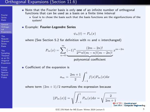
Orthogonal Expansions (Section 11.6)

Note that the Fourier basis is only one of an infinite number of orthogonalfunctions that can be used as a basis on a finite time interval

Goal is to chose the basis such that the basis functions are the eigenfunctions of thesystem!

Example: Fourier-Legendre Series

ψn(t) = Pn(x)

where (See Section 5.2 for definition with m and n interchanged)

Pm(x) =

∞∑n=0

(−1)n(2m− 2n)!

2mn!(m− n)!(m− 2n)!︸︷︷︸polynomial coefficient

xm−2n

Coefficient of the expansion is

am =2m+ 1

2

∫ 1

−1f (x)Pm(x)dx

where term (2m+ 1)/2 normalizes the expression because

‖Pm(x)‖ =

√∫ 1

−1Pm(x)dx =

√2

2m+ 1


Lecture 6

FourierSeriesBasis





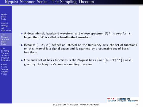
Nyquist-Shannon Series - The Sampling Theorem

A deterministic baseband waveform s(t) whose spectrum S(f ) is zero for |f |larger than W is called a bandlimited waveform.

Because (−W,W) defines an interval on the frequency axis, the set of functionson this interval is a signal space and is spanned by a countable set of basisfunctions.

One such set of basis functions is the Nyquist basis {sinc((t− T )/T

)} as is

given by the Nyquist-Shannon sampling theorem.


Lecture 6

FourierSeriesBasis





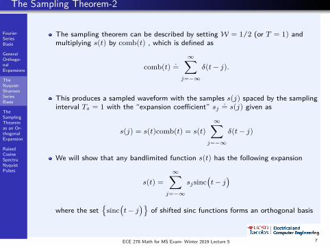
The Sampling Theorem-2

The sampling theorem can be described by setting W = 1/2 (or T = 1) andmultiplying s(t) by comb(t) , which is defined as

comb(t) .=

∞∑j=−∞

δ(t− j).

This produces a sampled waveform with the samples s(j) spaced by the samplinginterval Ts = 1 with the “expansion coefficient” sj

.= s(j) given as

s(j) = s(t)comb(t) = s(t)

∞∑j=−∞

δ(t− j)

We will show that any bandlimited function s(t) has the following expansion

s(t) =

∞∑j=−∞

sjsinc(t− j

)where the set

{sinc(t− j

)}of shifted sinc functions forms an orthogonal basis


Lecture 6

FourierSeriesBasis





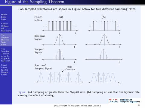
Figure of the Sampling TheoremTwo sampled waveforms are shown in Figure below for two different sampling rates.

. . .. . . . . . . . .

(a)

t

t

t

f

t

t

t

f

BasebandSignals

SampledSignals

Spectra of Sampled Signals

(b)Combsin Time

Rectfunction

Figure: (a) Sampling at greater than the Nyquist rate. (b) Sampling at less than the Nyquist rateshowing the effect of aliasing.


Lecture 6

FourierSeriesBasis





The Sampling Theorem as an Interpolation

Use the Fourier transform pair∞∑

j=−∞

δ(t− j)←→∞∑

j=−∞

δ(f − j)

orcomb(t)←→ comb(f ).

Now use the convolution property of the Fourier transform

s(t)h(t)←→ S(f )~H(f )

with the dual property

s(t)~ h(t)←→ S(f )H(f ).

Apply ths property to s(j) = s(t)comb(t) to give

s(t)comb(t)←→ S(f )~ comb(f )(s(t)comb(t)

)~ sinc(t)←→

(S(f )~ comb(f )

)rect(f )

where the Fourier transform pairs

rect(t)←→ sinc(f )sinc(t)←→ rect(f )

have been used.ECE 278 Math for MS Exam- Winter 2019 Lecture 5 9

Lecture 6

FourierSeriesBasis





Ideal Sampling

s(t)comb(t) ←→ S(f )~ comb(f ) (3)(s(t)comb(t)

)~ sinc(t) ←→

(S(f )~ comb(f )

)rect(f ) (4)

The left side of (3) is an infinite sequence of impulses with the area of the kthimpulse equal to the kth sample value.

The right side is the spectrum of the sampled waveform S(f )~ comb(f ) and isshown at the bottom of Figure 1 for two different sampling rates.

For the left set of curves in Figure 1a, multiplying the right by rect(f ), which isshown as a dashed line, recovers S(f ) because the support of S(f ) is[−1/2, 1/2] .

For this finite support, the images of the original spectrum S(f ) do not overlapin S(f )~ comb(f ).


Lecture 6

FourierSeriesBasis





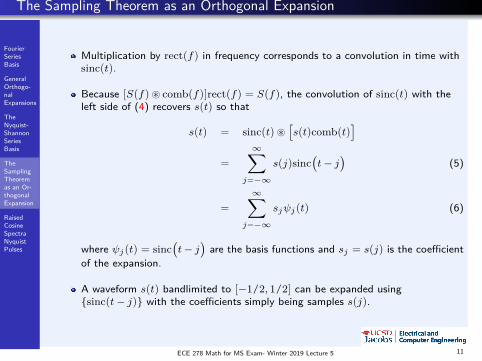
The Sampling Theorem as an Orthogonal Expansion

Multiplication by rect(f ) in frequency corresponds to a convolution in time withsinc(t).

Because [S(f )~ comb(f )]rect(f ) = S(f ), the convolution of sinc(t) with theleft side of (4) recovers s(t) so that

s(t) = sinc(t)~[s(t)comb(t)

]=

∞∑j=−∞

s(j)sinc(t− j

)(5)

=

∞∑j=−∞

sjψj(t) (6)

where ψj(t) = sinc(t− j

)are the basis functions and sj = s(j) is the coefficient

of the expansion.

A waveform s(t) bandlimited to [−1/2, 1/2] can be expanded using{sinc(t− j)} with the coefficients simply being samples s(j).


Lecture 6

FourierSeriesBasis





Orthogonality of Shifted Nyquist Pulses

Shifted sinc pulses are orthogonal because

ψn(t) ·ψm(t) =

∫ ∞−∞

sinc(t− n

)sinc(t−m

)dt

= δmn

For arbitrary sampling interval Ts , applying the scaling property of the Fouriertransform gives

s(t) =

∞∑j=−∞

sjψj(t) (7)

∞∑j=−∞

s(jTs)︸︷︷︸coefficient

sinc(

2Wt− j)︸︷︷︸

basis function

, (8)

where Ts = 1/2W.

In this way, the sequence of sinc functions is a sequence of interpolatingfunctions for a bandlimited signal.


Lecture 6

FourierSeriesBasis





Alaising

The images of the original signal spectrum S(f ) shown in Figure 1 are offset bythe sampling rate Rs = 1/Ts.

When Rs ≥ 2W, the images do not overlap. The minimum sampling rateRs = 2W is called the Nyquist rate.

When Rs is greater than or equal to the Nyquist rate, the images do not overlapand the original signal s(t) can be reconstructed as given by (7).

When the sampling rate is smaller than the Nyquist rate, the images of theoriginal signal spectrum S(f ) overlap.

This effect is called aliasing

Aliasing is a form of signal distortion that replicates frequency components in theoriginal signal at other frequencies in the reconstructed signal.


Lecture 6

FourierSeriesBasis





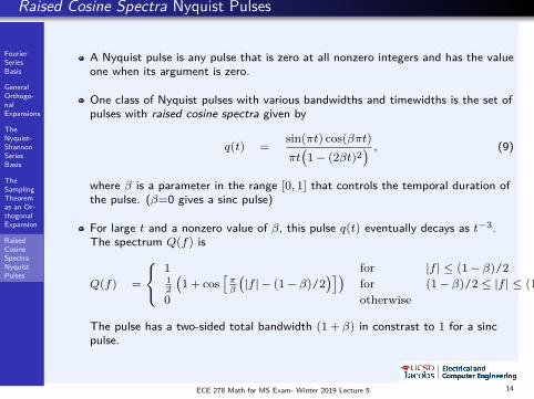
Raised Cosine Spectra Nyquist Pulses

A Nyquist pulse is any pulse that is zero at all nonzero integers and has the valueone when its argument is zero.

One class of Nyquist pulses with various bandwidths and timewidths is the set ofpulses with raised cosine spectra given by

q(t) =sin(πt) cos(βπt)πt(

1− (2βt)2) , (9)

where β is a parameter in the range [0, 1] that controls the temporal duration ofthe pulse. (β=0 gives a sinc pulse)

For large t and a nonzero value of β, this pulse q(t) eventually decays as t−3.The spectrum Q(f ) is

Q(f ) =

{1 for |f | ≤ (1− β)/212

(1 + cos

[πβ

(|f | − (1− β)/2

)])for (1− β)/2 ≤ |f | ≤ (1 + β)/2

0 otherwise.(10)

The pulse has a two-sided total bandwidth (1 + β) in constrast to 1 for a sincpulse.


Lecture 6

FourierSeriesBasis





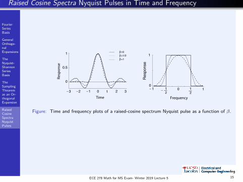
Raised Cosine Spectra Nyquist Pulses in Time and Frequency

�3 �2 �1 0 3 Time

0

0.5

1Re

spon

se

0

Frequency

0

1

Res

pons

e

β�1β�1/2β�0

1 21 2

1 2�

1� 1

Figure: Time and frequency plots of a raised-cosine spectrum Nyquist pulse as a function of β.


Lecture 6

FourierSeriesBasis





Choice of Sampling Basis

Shifted raised cosine spectra Nyquist pulses also form an orthogonal basis thatcan be used to represent a signal.

Choice depends bandwidth and computational complexity.

A sinc pulse has the smallest bandwidth of any basis function that can be used torepresent the signal.

However, expanding the signal using sinc pulses is computationally intensivebecause sinc(t) decays slowly as 1/t .

A large number of terms must be summed to accurately represent the signal inthe sinc expansion basis.

Noting that the sum of 1/n over n is divergent also alerts us to the concernexpressing the function using sincs is quite sensitive to instability or amplitudesaturation.

For other raised cosine pulses with β 6= 0, and large t the pulse decays as t−3

and thus it is easier to computationally represent this kind of basis function.

The cost is a larger bandwidth.


Lecture 6 - University of California, San Diego

Documents

Transcript of Lecture 6 - University of California, San Diego