MODELING OF ENERGETICAL PROPERTIES OF BIS-AZO COMPOUNDS. ROLE OF TAUTOMERIZATION

[email protected] ECRG VUW
Flowchart of NSGAII
21
Evaluate fitness
Evaluate fitness
Stop ?Return the final Pareto
Front
Generate initial population: size N
Yes No
Selection
Crossover
Mutation
Non-dominated Ranking
Select N individuals
Generate C
hild
ren P
opula
tio
n
Combine Parent and Children Populations
Elitism
Non-dominated Ranking and Crowding distance
[email protected] ECRG VUW
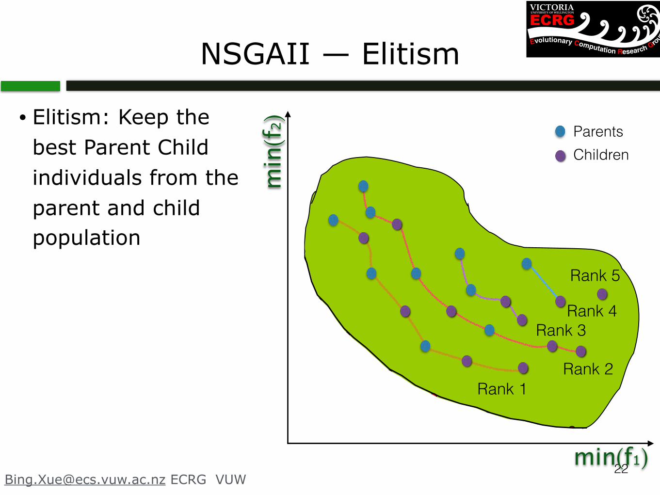
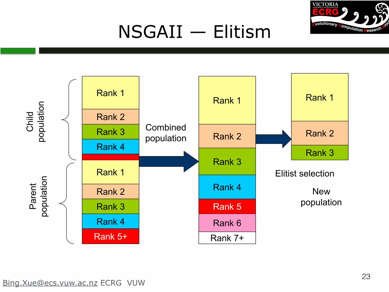
NSGAII — Elitism
• Elitism: Keep the best Parent Child individuals from the parent and child population
22min(f1)
min(f2)
Pareto optimal front
! Many optimal solutions! Usual approaches:
weighted sum strategy, ε-constraint modeling, Multi-objective GA
! Algorithm requirements: " Convergence" Spread
Min
f2
Min f1
Parents Children
Rank 3
Rank 2Rank 1
Rank 4
Rank 5
[email protected] ECRG VUW
NSGAII — Elitism
Elitism Process
Rank 1
Rank 2
Rank 3
Rank 4
Rank 1
Rank 2
Rank 3
Rank 5+
Rank 4
Chi
ld
popu
latio
nP
aren
t po
pula
tion
Rank 1
Rank 2
Rank 3
Rank 4
Rank 5
Rank 6
Rank 7+
Combined population
Rank 1
Rank 2
Rank 3
Elitist selection
New population
[email protected] ECRG VUW
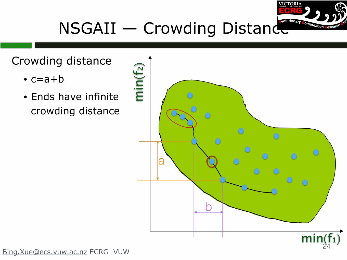
NSGAII — Crowding Distance
Crowding distance • c=a+b
• Ends have infinite crowding distance
24min(f1)
min(f2)
Pareto optimal front
! Many optimal solutions! Usual approaches:
weighted sum strategy, ε-constraint modeling, Multi-objective GA
! Algorithm requirements: " Convergence" Spread
Min
f2
Min f1
a
b
[email protected] ECRG VUW
SPEA2
• SPEA2: Improving the Strength Pareto Evolutionary Algorithm
• Compared to SPEA: • Fitness assignment scheme is used, which takes for each
individual into account how many individuals it dominates and it is dominated by. • Fitness is NOT based on objective function values
• Objective function values determine dominance relation
• A nearest neighbour density estimation technique is incorporated which allows a more precise guidance of the search process.
• A new archive truncation method guarantees the preservation of boundary solutions. 25

[email protected] ECRG VUW
Flowchart of SPEA2
26
Generate offsprings:
Binary tournament selection on Union,
then crossover, mutation
Combine Population and Archive to Union
Initial Population, and empty Archive (maxSize: S)
Copy non-dominated solutions in Population and
Archive to new Archive
Remove duplicates and dominated solutions in
Archive
26Stop ?
Return the Solutions in
Archive
YesArchive Truncation • delete if |Archive|>S • add dominated ones if |Archive|<S
No
En
viro
nm
en
tal se
lect
ion
Fitness Assignment: both Population and Archive

[email protected] ECRG VUW
Fitness Assignment• Each individual both dominating and dominated solutions are taken into account
• Fitness F(i) = Raw fitness R(i) +Density D(i)
• Nondominated: F(i) <1; dominated: F(i) >=1
• Raw fitness R(i) • Strength value S(i), representing the number of solutions (in both Population
and Archive) i dominates:
• Raw fitness R(i): is determined by the strengths of its dominators in both archive and population:
• Density D(i): • Additional density information is incorporated to discriminate between
individuals having identical raw fitness values.
• k-th nearest neighbour method: the inverse of the distance σik (in objective space) to the k-th nearest neighbour (in both archive and population) as the density estimate:
27
S(i) = |j|j 2 (Pop+Arch) ^ i � j|
R(i) =P
j2(Pop+Arch),j�i
S(j)
k =p
|Pop|+ |Arch|
solutions it dominates:1
S(i) = |{j | j ∈ Pt + P t ∧ i ≻ j}|
where | · | denotes the cardinality of a set, + stands for multiset union and the symbol≻ corresponds to the Pareto dominance relation. On the basis of the S values, the rawfitness R(i) of an individual i is calculated:
R(i) =∑
j∈Pt+P t,j≻i
S(j)
That is the raw fitness is determined by the strengths of its dominators in both archiveand population, as opposed to SPEA where only archive members are considered inthis context. It is important to note that fitness is to be minimized here, i.e., R(i) =0 corresponds to a nondominated individual, while a high R(i) value means that iis dominated by many individuals (which in turn dominate many individuals). Thisscheme is illustrated in Figure 1.
Although the raw fitness assignment provides a sort of niching mechanism based onthe concept of Pareto dominance, it may fail when most individuals do not dominateeach other. Therefore, additional density information is incorporated to discriminatebetween individuals having identical raw fitness values. The density estimation tech-nique used in SPEA2 is an adaptation of the k-th nearest neighbor method (Silverman1986), where the density at any point is a (decreasing) function of the distance to thek-th nearest data point. Here, we simply take the inverse of the distance to the k-thnearest neighbor as the density estimate. To be more precise, for each individual i thedistances (in objective space) to all individuals j in archive and population are calcu-lated and stored in a list. After sorting the list in increasing order, the k-th elementgives the distance sought, denoted as σk
i . As a common setting, we use k equal to thesquare root of the sample size (Silverman 1986), thus, k =
√
N + N . Afterwards, thedensityD(i) corresponding to i is defined by
D(i) =1
σki + 2
In the denominator, two is added to ensure that its value is greater than zero andthat D(i) < 1. Finally, adding D(i) to the raw fitness value R(i) of an individual iyields its fitness F (i):
F (i) = R(i) + D(i)
The run-time of the fitness assignment procedure is dominated by the density es-timator (O(M2 log M)), while the calculation of the S and R values is of complexityO(M2), whereM = N + N .
1This (and the following) formula slightly differs from the one presented in (Bleuler, Brack, Thiele, andZitzler 2001), where also individuals which have identical objective values contribute to the strength of anindividual.
7
[email protected] ECRG VUW
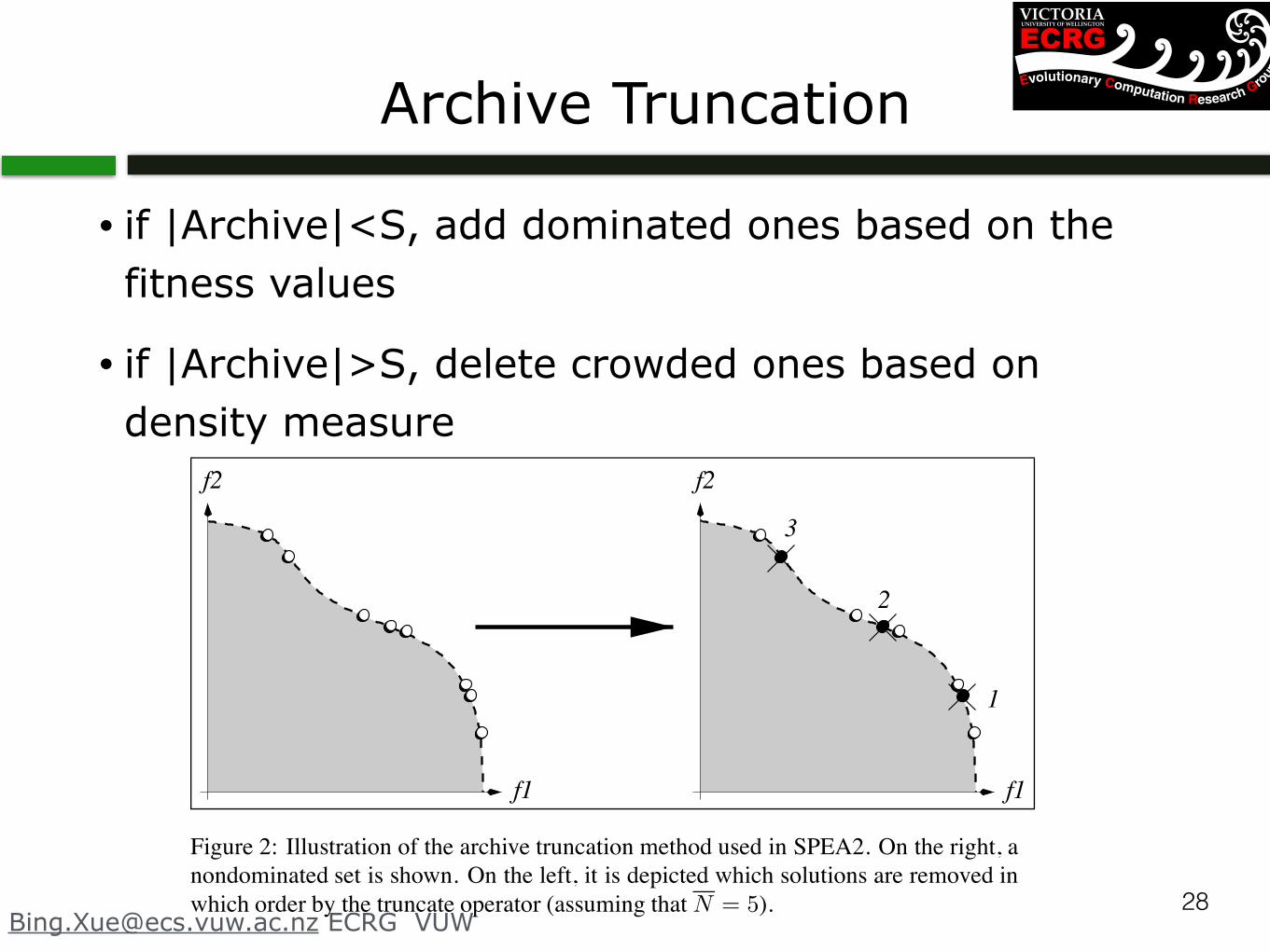
Archive Truncation
• if |Archive|<S, add dominated ones based on the fitness values
• if |Archive|>S, delete crowded ones based on density measure
28
3
2
1
f1
f2
f1
f2
Figure 2: Illustration of the archive truncation method used in SPEA2. On the right, anondominated set is shown. On the left, it is depicted which solutions are removed inwhich order by the truncate operator (assuming thatN = 5).
4.1 Test Problems and representation of solutionsThe test functions are summarized in Tab. 1, where both combinatorial and continuousproblems were chosen.
As combinatorial problems three instances of the knapsack problem were takenfrom (Zitzler and Thiele 1999), each with 750 items and 2, 3, and 4 objectives, respec-tively. For the random choice of the profit and weight values as well as the constrainthandling technique we refer to the original study. The individuals are represented asbit strings, where each bit corresponds to one decision variable. Recombination of twoindividuals is performed by one-point crossover. Point mutations are used where eachbit is flipped with a probability of 0.006, this value is taken using the guidelines derivedin (Laumanns, Zitzler, and Thiele 2001). The population size and the archive size wereset to 250 form = 2, to 300 form = 3, and to 400 form = 4.
In the continuous test functions different problems difficulties arise, for a discussionwe refer to (Veldhuizen 1999). Here, we enhanced the difficulty of each problem bytaking 100 decision variables in each case. For the Sphere Model (SPH-m) and forKursawe’s function (KUR) we also chose large domains in order to test the algorithms’ability to locate the Pareto-optimal set in a large objective space. For all continuousproblems, the individuals are coded as real vectors, where the SBX-20 operator is usedfor recombination and a polynomial distribution for mutation (Deb and Agrawal 1995).Furthermore, the population size and the archive size were set to 100.
The function SPH-m is a multi-objective generalization of the Sphere Model, asymmetric unimodal function where the isosurfaces are given by hyperspheres. TheSphere Model has been subject to intensive theoretical and empirical investigationswith evolution strategies, especially in the context of self-adaptation. In a multi-objective environment a two-variable version of it was used for empirical evaluationof VEGA (Schaffer 1985), while in (Rudolph 1998) it was used for theoretical con-
9