Fluctuations of the number of critical points of random trigonometric ...
24
ANALELE S ¸TIINT ¸ IFICE ALE UNIVERSIT ˘ AT ¸ II “AL.I. CUZA” DIN IAS ¸I (S.N.) MATEMATIC ˘ A, Tomul LIX, 2013, f.1 DOI: 10.2478/v10157-012-0019-6 FLUCTUATIONS OF THE NUMBER OF CRITICAL POINTS OF RANDOM TRIGONOMETRIC POLYNOMIALS * BY LIVIU I. NICOLAESCU Abstract. Denote by Zν the number of critical points of a random trigonometric polynomial of degree ≤ ν . We prove that as ν →∞ the expectation of Z ν is asymptotic to 2ν 3 5 while its variance is asymptotic to δ ∞ ν where δ ∞ ≈ 0.35. Mathematics Subject Classification 2010: 33B10, 42A61, 60D99. Key words: random functions, critical points, Kac-Rice formula. 1. Introduction A random trigonometric polynomial of degree ≤ ν is a trigonometric polynomial of the form η ν (t)= 1 √ 2π a 0 + 1 √ πν ν m=1 (a m cos mt + b m sin mt), t ∈ R/2πZ, where a m ,b m are independent normally distributed random variables with mean 0 and variance 1. The number Z ν of critical points of such a random polynomial is itself a random variable. The goal of this paper is to describe two important statis- tical quantities associated to this random quantity, namely its expectation, E ν , and its variance, V ν . We are particularly interested in the behavior of these quantities as the degree ν goes to infinity. In probabilistic parlance, η ν is a (stationary) Gaussian process on the unit circle R/2πZ and as ν →∞ this process approaches the singular process called white noise. * Invited paper Brought to you by | University of Notre Dame Authenticated | 129.74.204.221 Download Date | 4/3/13 11:12 PM
Transcript of Fluctuations of the number of critical points of random trigonometric ...
ANALELE STIINTIFICE ALE UNIVERSITATII “AL.I. CUZA” DIN IASI (S.N.)MATEMATICA, Tomul LIX, 2013, f.1DOI: 10.2478/v10157-012-0019-6
FLUCTUATIONS OF THE NUMBER OF CRITICAL POINTSOF RANDOM TRIGONOMETRIC POLYNOMIALS*
BY
LIVIU I. NICOLAESCU
Abstract. Denote by Z! the number of critical points of a random trigonometricpolynomial of degree ! !. We prove that as ! " # the expectation of Z! is asymptotic
to 2!!
35 while its variance is asymptotic to "!! where "! $ 0.35.
Mathematics Subject Classification 2010: 33B10, 42A61, 60D99.Key words: random functions, critical points, Kac-Rice formula.
1. Introduction
A random trigonometric polynomial of degree ! ! is a trigonometricpolynomial of the form
"!(t) =1"2#
a0 +1"#!
!!
m=1
(am cosmt+ bm sinmt), t # R/2#Z,
where am, bm are independent normally distributed random variables withmean 0 and variance 1.
The number Z! of critical points of such a random polynomial is itself arandom variable. The goal of this paper is to describe two important statis-tical quantities associated to this random quantity, namely its expectation,E! , and its variance, V! . We are particularly interested in the behavior ofthese quantities as the degree ! goes to infinity. In probabilistic parlance, "!is a (stationary) Gaussian process on the unit circle R/2#Z and as ! $ %this process approaches the singular process called white noise.
*Invited paper
Brought to you by | University of Notre DameAuthenticated | 129.74.204.221
Download Date | 4/3/13 11:12 PM
2 LIVIU I. NICOLAESCU 2
The main result of this paper shows that there exist (explicit) positiveconstants c1, c2 such that
E! & c1!, V! & c2! as ! $ %.
The above estimates imply an interesting concentration phenomenon.Suppose that we ask what are the odds that the number of critical pointsof a random trigonometric polynomial di!ers by more than 1% from theexpected number of critical points. In other words we ask what is theprobability of the event
|Z! ' E! | (E!
100.
The Chebyshev inequality shows
P (|Z! ' E! | ( 0.1E!) !V!
(0.01E!)2& 104c2
c21!as ! $ %.
Thus, the above event is highly unlikely if the degree ! is very large. Thisindicates that the highly oscillatory parts of a random trigonometric poly-nomials have a dominant e!ect in the creation of critical points. This isreminiscent of the classical Poincare phenomenon: the area of a large di-mensional round sphere tends to be concentrated on a narrow tube aroundan Equator1 of fixed and small codimension.
The statistics of the critical set of the above random function is identicalto the statistics of the zero set of the random function
$!(t) =d"!((t)
dt=
1"#!
!!
m=1
('mam sinmt+mbm cosmt).
Equivalently, consider the rescaled random function
"!(t) =1"#!3
n!
m=1
"mcm cos
"t
!
#+mdm sin
"t
!
##, t # ['#!,#!],
where cm, dm are independent random variables with identical standardnormal distribution, and the random variable
Z! := the number of zeros of "!(t) in the interval ['#!,#!].
1By Equator on a sphere centered at the origin of an Euclidean space we mean theintersection of the sphere with a vector subspace.
Brought to you by | University of Notre DameAuthenticated | 129.74.204.221
Download Date | 4/3/13 11:12 PM
3 RANDOM TRIGONOMETRIC POLYNOMIALS 3
Note that the expectation of Z! is precisely the expected number of criticalpoints of a random trigonometric polynomial in the space
T ! := span$cos(m%), sin(m%); m = 0, . . . !
%,
equipped with the inner product
(u, v) =
& 2"
0u(%)v(%)d%,
and Gaussian measure
d!(u) =1
(2#)dimT !
2
e!"u"2
2 du.
We let E(&), and respectively var(&), denote the expectation, and respec-tively the variance, of a random variable &. The random function "! is astationary Gaussian process with covariance kernel
R!(t) = E'"!(t)"!(0)
(=
1
#!3
!!
m=1
m2 cos
"mt
!
#.
The Rice formula, [2, Eq. (10.3.1)], implies that
E(Z!) = 2!
"'2(!)
'0(!)
# 12
,
where
'0(!) = R!(0) =1
#!3
!!
m=1
m2 and '2(!) = 'R""!(0) =
1
#!5
!!
m=1
m4.
This proves that
(1.1) E(Z!) & 2n
)3
5as n $ %.
The following is the main result of this paper.
Theorem 1.1. Set
'0 := lim!#$
'0(!) =1
3, '2 := lim
!#$'2(!) :=
1
5.
Brought to you by | University of Notre DameAuthenticated | 129.74.204.221
Download Date | 4/3/13 11:12 PM
4 LIVIU I. NICOLAESCU 4
Then for any t # R the limit lim!#$R!(t) exists, it is equal to
R$(t) :=1
t3
& t
0(2 cos (d( =
& 1
0'2 cos('t)d', )t # R,
and
(1.2) lim!#$
1
!var(Z!) = )$ :=
2
#
& $
!$
"f$(t)' '2
'0
#dt+ 2
*'2
'0,
where
f$(t) =('2
0 'R2$)'2 ' '0(R"
$)2
('20 'R2
$)32
+,1' *2$ + *$ arcsin *$
-,
and
*$ =R""
$('20 'R2
$) + (R"$)2R$
('20 'R2
$)'2 ' '0(R"$)2
.
Moreover, the constant )$ is positive.2
We should perhaps put this result in some perspective. Recently, Gran-ville and Wigman [4] have investigated the behavior of the number N! ofzeros of a random trigonometric polynomial of the form
P!(t) =1"#!
!!
m=1
'am cosmt+ bm sinmt
(, t # [0, 2#),
where am, bm are independent normally distributed random variables withmean 0 and variance 1. It is known that (see [3, 6])
E(N!) &)
2
3! as ! $ %,
but the authors show that a much more precise result is true. More precisely,they prove that there exists c > 0 such that as ! $ % the random variable
.N! =1"c!
'N! 'E(N!)
(
2Numerical experiments indicate that "! $ 0.35.
Brought to you by | University of Notre DameAuthenticated | 129.74.204.221
Download Date | 4/3/13 11:12 PM
5 RANDOM TRIGONOMETRIC POLYNOMIALS 5
converges to the standard Gaussian. Our strategy is inspired from [4] andwe believe that a central limit theorem is valid in the case of the statisticsof critical points as well. We plan to pursue this aspect elsewhere.
Let us observe that the space of trigonometric polynomials of degree! ! can be identified with the space UL spanned by the eigenfunctions ofthe Laplacian of S1 corresponding to eigenvalues ! L := !2. The estimate(1.1) can be rewritten as
(1.3) E(Z!) &)
3
5dimU!2 as ! $ %.
In [5] we proved a higher dimensional generalization of this estimate. Moreprecisely we have shown that for any m > 0 there exists an explicitpositive constant Cm > 0 such that for any compact, connected, smoothm-dimensional Riemann manifold if we denote by ZL the number of criticalpoints of a random linear combination of eigenfunctions of the Laplacian#g corresponding to eigenvalues ! L, then
E(ZL) & Cm dimUL as L $ %.
Theorem 1.1 suggests the following higher dimensional question: does thereexist a constant c > 1, possibly dependent on M and g, such that
1
cdimUL < var(ZL) < c dimUL as L $ % ?.
2. Proof of the main theorem
We follow a strategy inspired from [4]. The variance of Z! can be com-puted using the results in [2, §10.6]. We introduce the Gaussian field
!(t1, t2) :=
/
001
"!(t1)"!(t2)""!(t1)
""!(t2)
2
334 .
Its covariance matrix depends only on t = t2 ' t1. We have (compare with[4, Eq. (17)])
"(t) =
/
001
'0 R!(t) 0 R"!(t)
R!(t) '0 'R"!(t) 0
0 'R"!(t) '2 'r""!(t)
R"!(t) 0 'R""
!(t) '2
2
334 =:
5A BB† C
6.
Brought to you by | University of Notre DameAuthenticated | 129.74.204.221
Download Date | 4/3/13 11:12 PM
6 LIVIU I. NICOLAESCU 6
As explained in [6], to apply [2, §10.6] we only need that "(t) is non-degerate. This is established in the next result whose proof can be foundin Appendix A.
Lemma 2.1. The matrix "(t) is nonsingular if and only if t *# 2#!Z.
For any vector
x :=
/
001
x1x2x3x4
2
334 # R4
we set
pt1,t2(x) :=1
4#2(det")1/2e!
12 (!
#1x,x).
Then, the results in [2, §10.6] show that
(2.1) E(Z2! )'E(Z!)=
&
I!%I!
"&
R2|y1y2|·pt1,t2(0, 0, y1, y2)|dy1dy2|
#|dt1dt2|.
As in [4] we have
"(t)!1 =
5+ ++ $!1
6,$ = C 'B†A!1B.
More explicitly,
$ = C 'B†A!1B
=
5'2 'R""
!(t)'R""
!(t) '2
6
' 1
'20 'R!(t)2
50 'R"
!(t)R"
!(t) 0
6·5
'0 'R!(t)'R!(t) '0
6·5
0 R"!(t)
'R"!(t) 0
6
=
5'2 'R""
!
'R""! '2
6' (R"
!)2
'20 'R2
!
5'0 R!
R! '0
6= µ
51 '*'* 1
6,
where
µ = µ! =('2
0 'R2!)'2 ' '0(R"
!)2
'20 'R2
!, * = *! =
R""!('
20 'R2
!) + (R"!)
2R!
('20 'R2
!)'2 ' '0(R"!)
2.
We want to emphasize that in the above equalities the constants '0 and '2
do depend on !, although we have not indicated this in our notation.
Brought to you by | University of Notre DameAuthenticated | 129.74.204.221
Download Date | 4/3/13 11:12 PM
7 RANDOM TRIGONOMETRIC POLYNOMIALS 7
Remark 2.2. The nondegeneracy of " implies that µ!(t) *= 0 and|*!(t)| < 1, for all t *# 2#!Z.
We obtain as in [4, Eq. (24)]
det" = detA · det$ = µ2('20 'R2
!)(1' *2), $!1 =1
µ(1' *2)
51 ** 1
6.
We can now rewrite the equality (2.1) as (t = t2 ' t1)
E(Z2! )'E(Z!)
=
&
I!%I!
7&
R2|y1y2|e
! y21+2"y1y2+y222µ(1#"2)
|dy1dy2|4#2
8|dt1dt2|
µ,
('20 'R2
!)(1' *2)
=
&
I!%I!
7&
R2|y1y2|e
! y21+2"y1y2+y222(1#"2)
|dy1dy2|4#2
8µ|dt1dt2|,
('20 'R2
!)(1' *2).
From [1, Eq. (A.1)] we deduce that
&
R2|y1y2|e
! y21+2"y1y2+y222(1#"2)
|dy1dy2|4#2
=1' *2
#2
71 +
*,1' *2
arcsin *
8.
Hence
E(Z2! )'E(Z!) =
1
#2
&
I!%I!
µ
('20 'R2
!)12
+,1' *2 + * arcsin *
-|dt1dt2|
(2.2) =1
#2
&
I!%I!
('20 'R2
!)'2 ' '0(R"!)
2
('20 'R2
!)32
+,1' *2 + * arcsin *
-
9 :; <=:f!(t)
|dt1dt2|.
The function f!(t) = f!(t2 ' t1) is doubly periodic with periods 2#!, 2#!and we conclude that
(2.3) E([Z! ]2) := E(Z2! )'E(Z!) =
2!
#
& "!
!"!f!(t)dt.
We conclude that
var(Z!) = E([Z! ]2) +E(Z!)''E(Z!)
(2= E([Z! ]2)'
=E(Z!)
>2
=2!
#
& "!
!"!
"f!(t)'
'2
'0
#dt+ 2!
)'2
'0.
(2.4)
Brought to you by | University of Notre DameAuthenticated | 129.74.204.221
Download Date | 4/3/13 11:12 PM
8 LIVIU I. NICOLAESCU 8
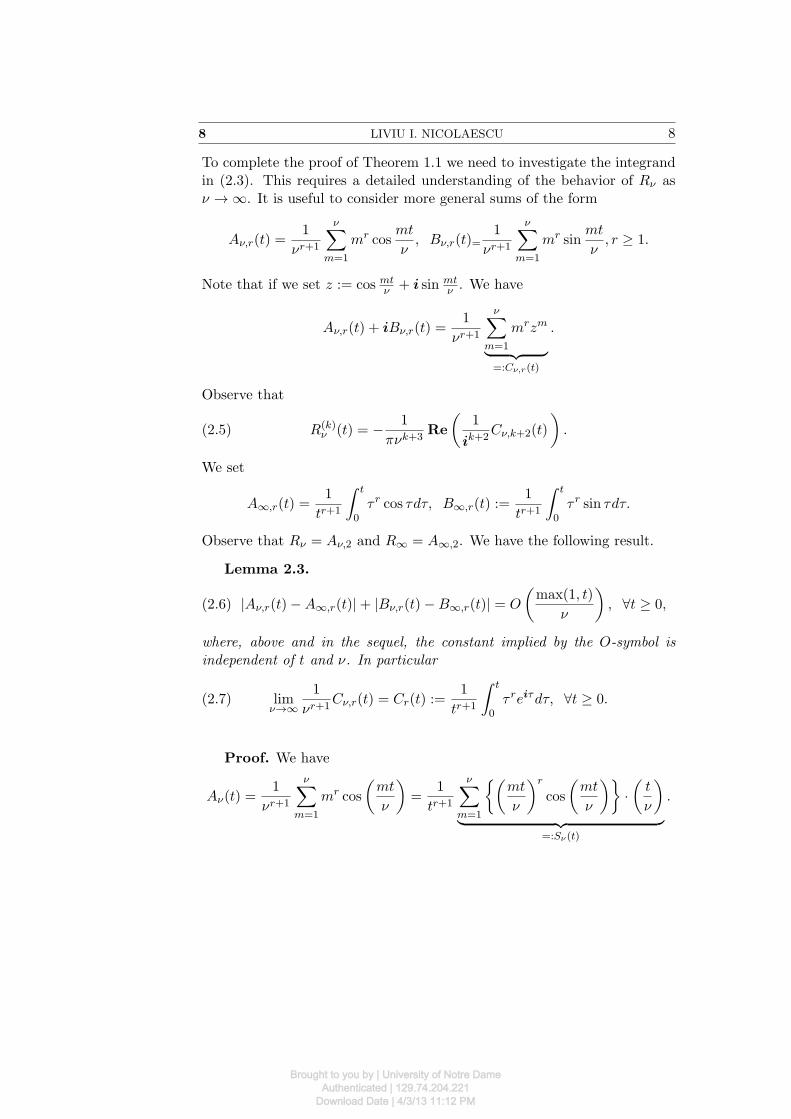
To complete the proof of Theorem 1.1 we need to investigate the integrandin (2.3). This requires a detailed understanding of the behavior of R! as! $ %. It is useful to consider more general sums of the form
A!,r(t) =1
!r+1
!!
m=1
mr cosmt
!, B!,r(t)=
1
!r+1
!!
m=1
mr sinmt
!, r ( 1.
Note that if we set z := cos mt! + i sin mt
! . We have
A!,r(t) + iB!,r(t) =1
!r+1
!!
m=1
mrzm
9 :; <=:C!,r(t)
.
Observe that
(2.5) R(k)! (t) = ' 1
#!k+3Re
"1
ik+2C!,k+2(t)
#.
We set
A$,r(t) =1
tr+1
& t
0( r cos (d(, B$,r(t) :=
1
tr+1
& t
0( r sin (d(.
Observe that R! = A!,2 and R$ = A$,2. We have the following result.
Lemma 2.3.
(2.6) |A!,r(t)'A$,r(t)|+ |B!,r(t)'B$,r(t)| = O
"max(1, t)
!
#, )t ( 0,
where, above and in the sequel, the constant implied by the O-symbol isindependent of t and !. In particular
(2.7) lim!#$
1
!r+1C!,r(t) = Cr(t) :=
1
tr+1
& t
0( rei#d(, )t ( 0.
Proof. We have
A!(t) =1
!r+1
!!
m=1
mr cos
"mt
!
#=
1
tr+1
!!
m=1
?"mt
!
#r
cos
"mt
!
#@·"t
!
#
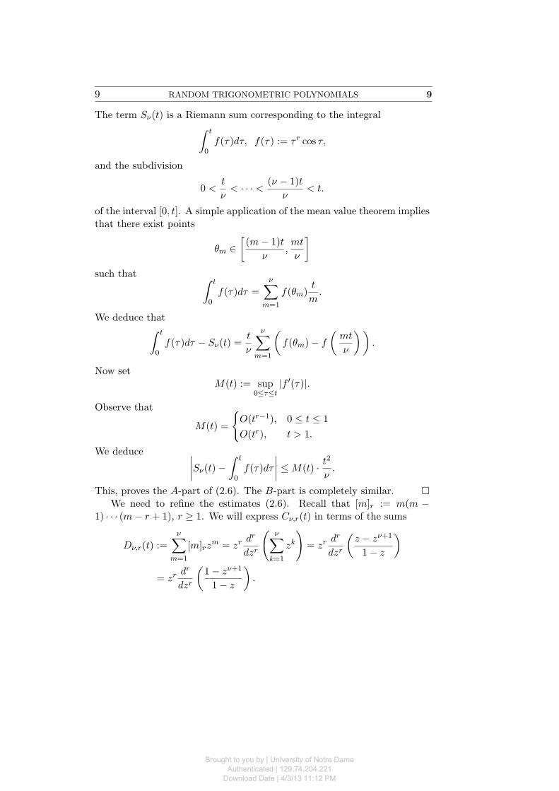
9 :; <=:S!(t)
.
Brought to you by | University of Notre DameAuthenticated | 129.74.204.221
Download Date | 4/3/13 11:12 PM
9 RANDOM TRIGONOMETRIC POLYNOMIALS 9
The term S!(t) is a Riemann sum corresponding to the integral& t
0f(()d(, f(() := ( r cos (,
and the subdivision
0 <t
!< · · · < (! ' 1)t
!< t.
of the interval [0, t]. A simple application of the mean value theorem impliesthat there exist points
%m #5(m' 1)t
!,mt
!
6
such that & t
0f(()d( =
!!
m=1
f(%m)t
m.
We deduce that& t
0f(()d( ' S!(t) =
t
!
!!
m=1
"f(%m)' f
"mt
!
##.
Now setM(t) := sup
0&#&t|f "(()|.
Observe that
M(t) =
AO(tr!1), 0 ! t ! 1
O(tr), t > 1.
We deduce BBBBS!(t)'& t
0f(()d(
BBBB ! M(t) · t2
!.
This, proves the A-part of (2.6). The B-part is completely similar. !We need to refine the estimates (2.6). Recall that [m]r := m(m '
1) · · · (m' r + 1), r ( 1. We will express C!,r(t) in terms of the sums
D!,r(t) :=!!
m=1
[m]rzm = zr
dr
dzr
7!!
k=1
zk8
= zrdr
dzr
"z ' z!+1
1' z
#
= zrdr
dzr
"1' z!+1
1' z
#.
Brought to you by | University of Notre DameAuthenticated | 129.74.204.221
Download Date | 4/3/13 11:12 PM
10 LIVIU I. NICOLAESCU 10
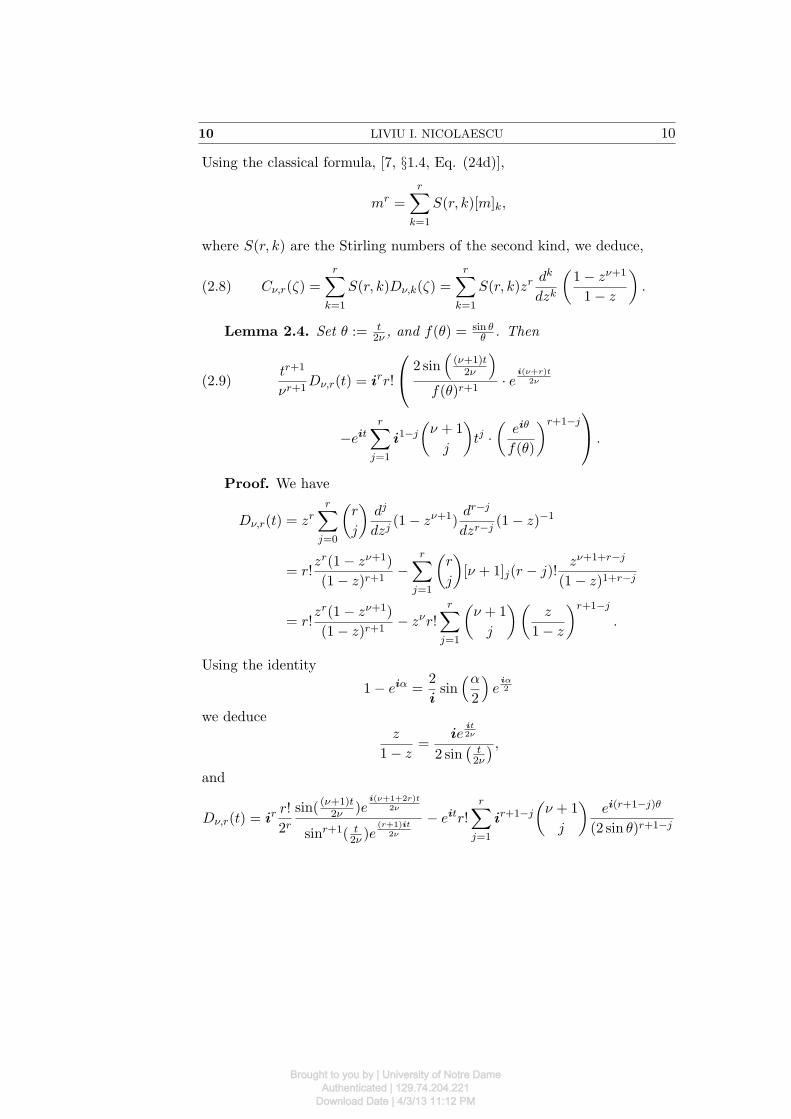
Using the classical formula, [7, §1.4, Eq. (24d)],
mr =r!
k=1
S(r, k)[m]k,
where S(r, k) are the Stirling numbers of the second kind, we deduce,
(2.8) C!,r(&) =r!
k=1
S(r, k)D!,k(&) =r!
k=1
S(r, k)zrdk
dzk
"1' z!+1
1' z
#.
Lemma 2.4. Set % := t2! , and f(%) = sin $
$ . Then
tr+1
!r+1D!,r(t) = irr!
C
D2 sin
+(!+1)t
2!
-
f(%)r+1· e
i(!+r)t2!(2.9)
'eitr!
j=1
i1!j
"! + 1
j
#tj ·"
ei$
f(%)
#r+1!jE
F .
Proof. We have
D!,r(t) = zrr!
j=0
"r
j
#dj
dzj(1' z!+1)
dr!j
dzr!j(1' z)!1
= r!zr(1' z!+1)
(1' z)r+1'
r!
j=1
"r
j
#[! + 1]j(r ' j)!
z!+1+r!j
(1' z)1+r!j
= r!zr(1' z!+1)
(1' z)r+1' z!r!
r!
j=1
"! + 1
j
#"z
1' z
#r+1!j
.
Using the identity
1' ei% =2
isin++2
-e
i#2
we deducez
1' z=
ieit2!
2 sin'
t2!
( ,
and
D!,r(t) = irr!
2rsin( (!+1)t
2! )ei(!+1+2r)t
2!
sinr+1( t2! )e
(r+1)it2!
' eitr!r!
j=1
ir+1!j
"! + 1
j
#ei(r+1!j)$
(2 sin %)r+1!j
Brought to you by | University of Notre DameAuthenticated | 129.74.204.221
Download Date | 4/3/13 11:12 PM
11 RANDOM TRIGONOMETRIC POLYNOMIALS 11
= irr!
C
D2 sin
+(!+1)t
2!
-
(2 sin %)r+1 · ei(!+r)t
2! ' eitr!
j=1
i1!j
"! + 1
j
#"ei$
2 sin %
#1+r!jE
F .
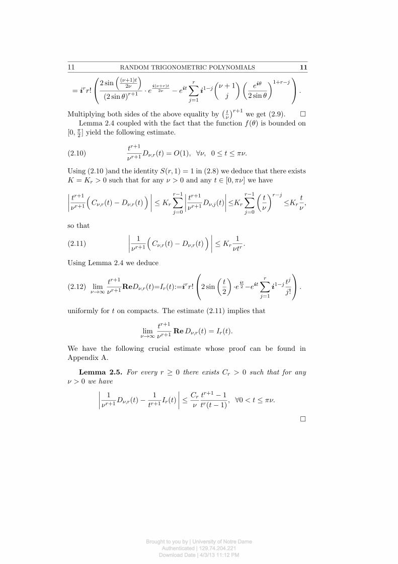
Multiplying both sides of the above equality by't!
(r+1we get (2.9). !
Lemma 2.4 coupled with the fact that the function f(%) is bounded on[0, "2 ] yield the following estimate.
(2.10)tr+1
!r+1D!,r(t) = O(1), )!, 0 ! t ! #!.
Using (2.10 )and the identity S(r, 1) = 1 in (2.8) we deduce that there existsK = Kr > 0 such that for any ! > 0 and any t # [0,#!] we have
BBBBtr+1
!r+1
+C!,r(t)'D!,r(t)
- BBBB ! Kr
r!1!
j=0
BBBBtr+1
!r+1D!,j(t)
BBBB!Kr
r!1!
j=0
"t
!
#r!j
!Krt
!,
so that
(2.11)
BBBB1
!r+1
+C!,r(t)'D!,r(t)
- BBBB ! Kr1
!tr.
Using Lemma 2.4 we deduce
(2.12) lim!#$
tr+1
!r+1ReD!,r(t)=Ir(t):=irr!
C
D2 sin
"t
2
#·e
it2 'eit
r!
j=1
i1!j tj
j!
E
F .
uniformly for t on compacts. The estimate (2.11) implies that
lim!#$
tr+1
!r+1ReD!,r(t) = Ir(t).
We have the following crucial estimate whose proof can be found inAppendix A.
Lemma 2.5. For every r ( 0 there exists Cr > 0 such that for any! > 0 we have
BBBB1
!r+1D!,r(t)'
1
tr+1Ir(t)
BBBB !Cr
!
tr+1 ' 1
tr(t' 1), )0 < t ! #!.
!
Brought to you by | University of Notre DameAuthenticated | 129.74.204.221
Download Date | 4/3/13 11:12 PM
12 LIVIU I. NICOLAESCU 12
Using Lemma 2.5 in (2.11) we deduce
(2.13a)
BBBB1
!r+1C!,r(t)'
1
tr+1Ir(t)
BBBB !Cr
!
tr+1 ' 1
tr(t' 1), )0 < t ! #!.
(2.13b) Ir(t) = tr+1Cr(t) =
& t
0( rei#d(.
Using (2.6) and (2.13a) we deduce that for any nonnegative integer r thereexists a positive constant K = Kr > 0 such that
(2.14) |C!,r(t)' Cr(t)| !Kr
!
tr+1 ' 1
tr(t' 1).
Coupling the above estimates with (2.6) we deduce
(2.15) C!,r(t) = Cr(t) +O
"1
!
#, )0 ! t ! !,
where the constant implied by the symbol O depends on k, but it is inde-pendent of !. The last equality coupled with (2.5) implies that
(2.16) R(k)! (t) = R(k)
$ (t) +O
"1
!
#, )0 ! t ! !.
We deduce that, for any t > 0 we have
lim!#$
f!(t) = f$(t),
where f! is the function defined in (2.2), while
(2.17) f$(t) =('2
0 'R2$)'2 ' '0(R"
$)2
('20 'R2
$)32
+,1' *2$ + *$ arcsin *$
-,
where
'0 = '0(%) = lim!#$
'0(!) =1
3, '2 = lim
!#$'2(!) =
1
5,
*$(t) = lim!#$
*!(t) =R""
$('20 'R2
$) + (R"$)2R$
('20 'R2
$)'2 ' '0(R"$)2
.
We have the following result whose proof can be found in Appendix A.
Brought to you by | University of Notre DameAuthenticated | 129.74.204.221
Download Date | 4/3/13 11:12 PM
13 RANDOM TRIGONOMETRIC POLYNOMIALS 13
Lemma 2.6.
(2.18a) |R$(t)| < R$(0), |R""$(t)| < |R""
$(0)|, )t > 0,
(2.18b) R$(t), R"$(t), R""
$(t) = O
"1
t
#as t $ %.
(2.18c) ('20 'R2
$)'2 ' '0(R"$)2 > 0, )t > 0.
(2.18d)R$(t) = 1
3 ' 110 t
2 + 1168 t
4 +O(t6),R"
$(t) = '15 t+
142 t
3 +O(t5), as t $ 0.
We set)(t) := max(t, 1), t ( 0.
We find it convenient to introduce new functions
G!(t) :=1
R!(0)R!(t) =
1
'0(!)R!(t), H!(t) =
1
R""!(0)
R""!(t) = ' 1
'2(!)R""
!(t).
Using these notations we can rewrite (2.18c) as
(2.19) (1'G2$)' '0
'2(G"
$)2
9 :; <=:&(t)
> 0, )t > 0.
The equalities (2.18d) imply that
(2.20) "(t) =3
4375t4 +O(t6), )|t| , 1.
Then
f!(t) ='2(!)
'0(!)- C!(t)-
+,1' *2! + *! arcsin *!
-,
where
C!(t) :=(1'G!(t)2)' '0(!)
'2(!))(G"
!(t))2
(1'G!(t)2)3/2,
and
*! =R""
!('0(!)2 'R2!) + (R"
!)2R!
('20(!)'R2
!)'2(!)' '0(R"!)
2=
'H!(1'G2!) +
'0(!)'2(!)
(G"!)
2G!
(1'G2!)'
'0(!)'2(!)
(G"!)
2.
Brought to you by | University of Notre DameAuthenticated | 129.74.204.221
Download Date | 4/3/13 11:12 PM
14 LIVIU I. NICOLAESCU 14
Lemma 2.7. Let , # (0, 1). Then
C!(t) = O(t), )0 ! t ! !!(,
where the constant implied by O-symbol is independent of ! and t # [0, !!(),but it could depend on ,.
Proof. Observe that for t # [0, !!(] we have
G!(t) = 1' '2(!)
2'0(!)t2 +O(t4), G"
!(t) = ''2(!)
'0(!)t+O(t3)
so that'1'G!(t)
2(!3/2
=
"'2(!)
'0(!)t
#!3
- (1 +O(t) ),
and
(1'G!(t)2)' '0(!
'2(!)(G"
!) = O(t4)
so that C!(t) = O(t). !
Lemma 2.8. Let , # (0, 1),
"(t) := (1'G2!)'
'0
'2(G"
!)2 and -(t) = 1'G$(t)2.
Then as ! $ % and t > !!( we have
(2.21) C! = C$ -"1 +O
"(G"
$)2
!"(t)+
1
!-(t))(t)+
1
!)(t)"(t)+
1
!2"(t)
##,
and(2.22)
C!(t)=C$(t)+O
"(G"
$)2
!-(t)3/2+
"(t)
!)(t)-(t)3/2+
1
!)(t)-(t)3/2+
1
!2-(t)3/2
#,
uniformly for t > !!(.
Proof. Observe that
(2.23) G2! =
"G$ +O
"1
!
##2(2.18b)= G2
$ +O
"1
!)(t)
#,
Brought to you by | University of Notre DameAuthenticated | 129.74.204.221
Download Date | 4/3/13 11:12 PM
15 RANDOM TRIGONOMETRIC POLYNOMIALS 15
so that
1'G$(t)2(t) ='1'G$(t)2
("1 +O
"1
!)(t)-(t)
##.
For t > !!( we have
1
!)(t)-(t)= O
"1
!1!(
#= o(1) uniformly in t > !!( as ! $ %.
Hence
'1'G2
!
(!3/2='1'G2
$(!3/2
"1 +O
"1
!)(t)-(t)
##,
-(t) := 1'G2$(t).(2.24)
Next observe that
'0(!) =B3(! + 1)
3!3=
1
3+ !!1 +O(!!2),(2.25)
'2(!) =B5(! + 1)
5!5=
1
5+ !!1 +O(!!2)
and'0(!)
'2(!)=
13 + !!1 +O(!!2)15 + !!1 +O(!!2)
=5
3' 10
3!!1 +O(!!2).
Using (2.23) and the above estimate we deduce
(1'G!(t)2)' '0(!)
'2(!))(G"
!)2
= (1'G2$)' '0
'2(G"
$)2
9 :; <&(t)
+10
3!(G"
$)2 +O
"1
!)(t)
#+O
"1
!2
#(2.26)
=
"(1'G2
$)' '0
'2(G"
$)2#·"1+O
"(G"
$)2
!"(t)+
1
!)(t)"(t)+
1
!2"(t)
##.
Using (2.24) we deduce (2.21). The estimate (2.22) follows from (2.21) byinvoking the definitions of -(t) and "(t). !
Brought to you by | University of Notre DameAuthenticated | 129.74.204.221
Download Date | 4/3/13 11:12 PM
16 LIVIU I. NICOLAESCU 16
Lemma 2.9. Let , # (0, 14). Then
*!=*$ +O
"1
!"(t)+
(G"$)2
!"(t))(t)+
1
!)(t)2+
1
!)(t)2"(t)+
1
!2"(t))(t)
#,(2.27)
)t > !!(,
where the constant implied by O-symbol is independent of ! and t > !!(,but it could depend on ,.
Proof. The estimates (2.18b), (2.18d) and (2.20) imply that for t > !!(
we have(G"
$)2
!"(t)+
1
!)(t)"(t)+
1
!2"(t)= O(
1
!1!4() = o(1),
uniformly in t > !!(. We conclude from (2.26) that
+(1'G!(t)
2)' '0(!)
'2(!))(G"
!)2-!1
=
"'1'G2
$(' '0
'2(G"
$)2#!1
-"1 +O
"(G"
$)2
!"(t)+
1
!)(t)"(t)+
1
!2"(t)
##.(2.28)
Since H! = H$ +O(!!1) we deduce
'H!(1'G!)2+
'0(!)
'2(!)(G"
!)2G!='H$(1'G$)2+
'0
'2(G"
$)2G$ +O
"1
!
#.
Recalling that
*! ='H!(1'G2
!) +'0(!)'2(!)
(G"!)
2G!
(1'G2!)'
'0(!)'2(!)
(G"!)
2
and 'H$(1 ' G$)2 + '0
'2(G"
$)2G$ = O()!1) we see that (2.27) follows
from (2.28). !Consider the function
A(u) =,
1' u2 + u arcsinu, |u| ! 1.
Observe that
(2.29a)dA
du= O(1), )|u| ! 1,
Brought to you by | University of Notre DameAuthenticated | 129.74.204.221
Download Date | 4/3/13 11:12 PM
17 RANDOM TRIGONOMETRIC POLYNOMIALS 17
(2.29b)dA
du= arcsinu = O(u) as u $ 0.
Now fix an exponent , # (0, 14). We discuss separately two cases.
1. If !k < t < #!. Then in this range we have
1
), *$ = O(t!1), *! = *$ + o(1),
1
"(t)= O(1),
and using (2.29b) and (2.27) we deduce
A(*!) = A(*$) +A"(*$)(*! ' *$) +O'(*! ' *$)2
((2.30)
= A(*$) +O
"1
t!+
1
!2
#.
2. !!( < t < !(. The equality (2.20) shows that in this range we have
1
"(t)= O(!!4(),
1
)(t)= O(1)
so that and (2.27) implies that
*! ' *$ = O
"1
!1!4k
#.
Using (2.29a) we deduce
(2.31) A(*!)'A(*$) = O
"1
!1!4k+
1
!1!4()(t)2+
1
!2!8()(t)
#.
Set
#! := C!A(*!)' C$A(*$), q! :=
"'2(!)
'0(!)
#, q$ =
"'2
'0
#.
Then using (2.25) we deduce that
q! ' q$ =6
5!!1 +O(!!2), q! = q$
'1 + 2!!1 +O(!!2)
(.
Then +f!(t)' q!
-'+f$(t)' q$
-=
Brought to you by | University of Notre DameAuthenticated | 129.74.204.221
Download Date | 4/3/13 11:12 PM
18 LIVIU I. NICOLAESCU 18
= q!'C$A$(*$)' 1 +#!
(' q$
'C$A(*$)' 1
(
='q! ' q$)
'C$A(*$)' 1
(+ q$#! .
To prove (1.2) we need to prove the following equality.
'q! ' q$)
& "!
0
'C$(t)A(*$(t))' 1
(dt,(2.32)
q$
& "!
0#!(t)dt = o(1) as ! $ %.
We can dispense easily of the first integral above since C$(t)A(*$(t)) ' 1is absolutely integrable on [0,%) and q! ' q$ = O(!!1).
The second integral requires a bit of work. More precisely, we will showthe following result.
Lemma 2.10. If 0 < , < 15 , then
(2.33)
& !#$
0#!(t)dt,
& !$
!#$#!(t)dt,
& "!
!$#!(t)dt = o(1) as ! $ %.
Proof. We will discuss each of the three cases separately.
1. 0 < t < !!(. The easiest way to prove thatG !#$
0 #!(t)dt $ 0 is to showthat
C!(t)A(*!(t)) = O(1), 0 < t < !!k.
This follows using Lemma 2.7 and observing that the function A(u) isbounded.
2. !!( < t < !(. In this range we have
1
"= O(!!4(),
1
-(t)= O(!!2(),
1
)(t)= O(1), G"
$(t) = O(1).
Using (2.22), (2.31) we deduce
C!(t) = C$(t) +O
"1
!1!3(
#, A(*!) = A(*$) +O
"1
!1!4(
#.
Hence
#! = O
"1
!1!4(
#and
& !$
!#$#!(t)dt = O
"1
!1!5(
#= o(1).
Brought to you by | University of Notre DameAuthenticated | 129.74.204.221
Download Date | 4/3/13 11:12 PM
19 RANDOM TRIGONOMETRIC POLYNOMIALS 19
3. !( < t < #!. For these values of t we have
"(t),1
"(t)= O(1),
1
)(t)= O(t!1).
Using (2.22) and (2.30) we deduce
C!(t) = C$(t) +O
"1
!t+
1
!2
#, A(*!) = A(*$) +O
"1
!t+
1
!2
#
so that
#!(t) = O
"1
!t+
1
!2
#,
& "!
!#$#!(t) dt = O
"1
!+
log !
!
#= o(1).
!The fact that )$ defined as in (1.2) is positive follows by arguing exactly
as in [4, §3.2]. This completes the proof of Theorem 1.1.
Remark 2.11. The proof of Lemma 2.10 shows that for any . > 0 wehave
(2.34) var(Z!) = !)$ +O(!)) as ! $ %.
Numerical experiments suggest that )$ . 0.35.
A. Some elementary estimates
Proof of Lemma 2.1. Consider the complex valued random process
F!(t) :=1"#!3
!!
m=1
mzmeimt! , zm = cm ' idm.
The covariance function of this process is
R!(t) = E'F!(t)F!(0)
(=
1
#!3
!!
m=1
m2eimt! .
Observe that ReF! = "! . Note that the spectral measure of the processF! is
d/! =1
#!3
!!
m=1
m2)m!,
Brought to you by | University of Notre DameAuthenticated | 129.74.204.221
Download Date | 4/3/13 11:12 PM
20 LIVIU I. NICOLAESCU 20
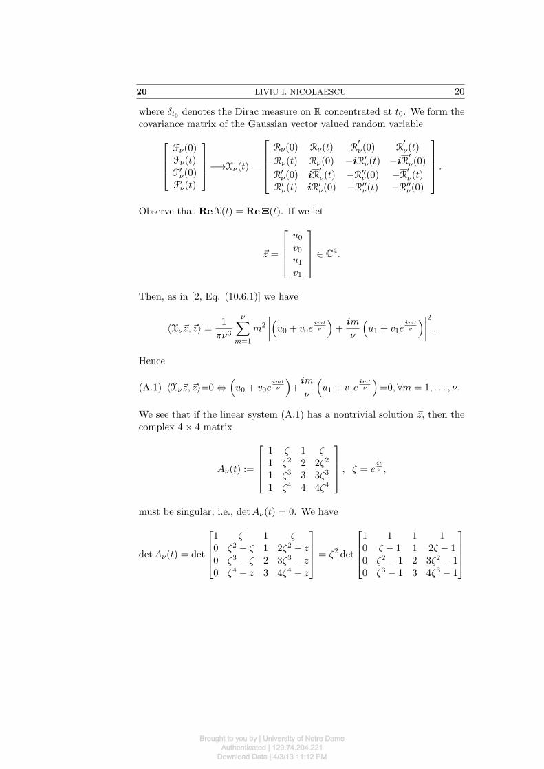
where )t0 denotes the Dirac measure on R concentrated at t0. We form thecovariance matrix of the Gaussian vector valued random variable
/
001
F!(0)F!(t)F"!(0)
F"!(t)
2
334'$X!(t) =
/
0001
R!(0) R!(t) R"!(0) R
"!(t)
R!(t) R!(0) 'iR"!(t) 'iR
"!(0)
R"!(0) iR
"!(t) 'R""
!(0) 'R"!(t)
R"!(t) iR"
!(0) 'R""!(t) 'R""
!(0)
2
3334.
Observe that ReX(t) = Re"(t). If we let
0z =
/
001
u0v0u1v1
2
334 # C4.
Then, as in [2, Eq. (10.6.1)] we have
/X!0z, 0z0 =1
#!3
!!
m=1
m2
BBBB+u0 + v0e
imt!
-+
im
!
+u1 + v1e
imt!
-BBBB2
.
Hence
(A.1) /X!0z, 0z0=0 1+u0 + v0e
imt!
-+im
!
+u1 + v1e
imt!
-=0, )m = 1, . . . , !.
We see that if the linear system (A.1) has a nontrivial solution 0z, then thecomplex 4- 4 matrix
A!(t) :=
/
001
1 & 1 &1 &2 2 2&2
1 &3 3 3&3
1 &4 4 4&4
2
334 , & = eit! ,
must be singular, i.e., detA!(t) = 0. We have
detA!(t) = det
/
001
1 & 1 &0 &2 ' & 1 2&2 ' z0 &3 ' & 2 3&3 ' z0 &4 ' z 3 4&4 ' z
2
334 = &2 det
/
001
1 1 1 10 & ' 1 1 2& ' 10 &2 ' 1 2 3&2 ' 10 &3 ' 1 3 4&3 ' 1
2
334
Brought to you by | University of Notre DameAuthenticated | 129.74.204.221
Download Date | 4/3/13 11:12 PM
21 RANDOM TRIGONOMETRIC POLYNOMIALS 21
= &2 det
/
1& ' 1 1 2& ' 1&2 ' 1 2 3&2 ' 1&3 ' 1 3 4&3 ' 1
2
4 = &2 det
/
1& ' 1 1 &&2 ' 1 2 2&2
&3 ' 1 3 3&3
2
4
= &3 det
/
1& ' 1 1 1&2 ' 1 2 2&&3 ' 1 3 3&2
2
4 = & det
/
1& ' 1 1 0&2 ' 1 2 2&2 ' 2&3 ' 1 3 3&3 ' 3
2
4
= &3 det
/
1& ' 1 1 0
&2 ' 2& + 1 0 2&2 ' 2&3 ' 3& + 2 0 3&3 ' 3
2
4
= &3 det
/
1& ' 1 1 0
(& ' 1)2 0 2(& ' 1)(& + 1)&3 ' 3& + 2 0 3&3 ' 3
2
4
= &3(& ' 1) det
/
1& ' 1 1 0(& ' 1) 0 2(& + 1)
(& ' 1)2(& + 1) 0 3(& ' 1)(&2 + & + 1)
2
4
= &3(& ' 1)3 det
/
11 1 01 0 2(& + 1)
& + 1) 0 3(&2 + & + 1)
2
4
= '&3(& ' 1)3'3(&2 + & + 1)' 2(&2 + 2& + 1)
(
= '&3(& ' 1)3(&2 ' & ' 1).
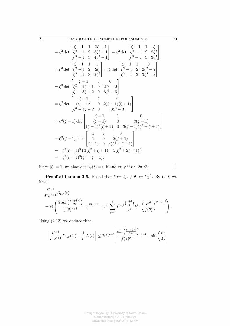
Since |&| = 1, we that detA!(t) = 0 if and only if t # 2#!Z.
Proof of Lemma 2.5. Recall that % := t2! , f(%) :=
sin $$ . By (2.9) we
have
tr+1
ir!r+1D!,r(t)
= r!
C
D2 sin
+(!+1)t
2!
-
f(%)r+1· e
i(!+r)t2! ' eit
r!
j=1
i1!j
'!+1j
(
!jtj ·"
ei$
f(%)
#r+1!jE
F .
Using (2.12) we deduce that
BBBBtr+1
ir!r+1D!,r(t))'
1
irIr(t)
BBBB ! 2r!tr+1
BBBBBB
sin+(!+1)t
2!
-
f(%)r+1eir$ ' sin
"t
2
#BBBBBB
Brought to you by | University of Notre DameAuthenticated | 129.74.204.221
Download Date | 4/3/13 11:12 PM
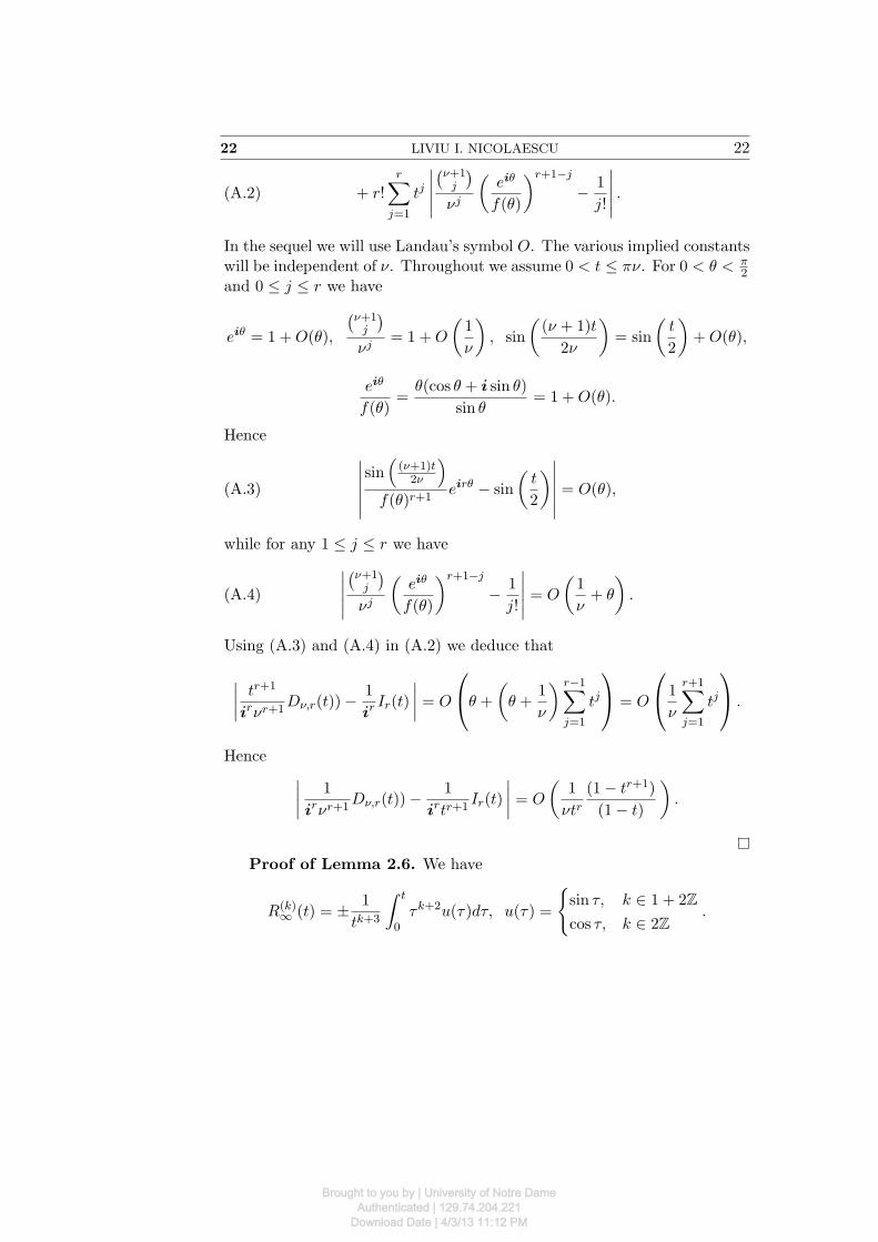
22 LIVIU I. NICOLAESCU 22
+ r!r!
j=1
tj
BBBBB
'!+1j
(
!j
"ei$
f(%)
#r+1!j
' 1
j!
BBBBB .(A.2)
In the sequel we will use Landau’s symbol O. The various implied constantswill be independent of !. Throughout we assume 0 < t ! #!. For 0 < % < "
2and 0 ! j ! r we have
ei$ = 1 +O(%),
'!+1j
(
!j= 1 +O
"1
!
#, sin
"(! + 1)t
2!
#= sin
"t
2
#+O(%),
ei$
f(%)=
%(cos % + i sin %)
sin %= 1 +O(%).
Hence
(A.3)
BBBBBB
sin+(!+1)t
2!
-
f(%)r+1eir$ ' sin
"t
2
#BBBBBB= O(%),
while for any 1 ! j ! r we have
(A.4)
BBBBB
'!+1j
(
!j
"ei$
f(%)
#r+1!j
' 1
j!
BBBBB = O
"1
!+ %
#.
Using (A.3) and (A.4) in (A.2) we deduce that
BBBBtr+1
ir!r+1D!,r(t))'
1
irIr(t)
BBBB = O
C
D% +
"% +
1
!
# r!1!
j=1
tj
E
F = O
C
D1
!
r+1!
j=1
tj
E
F .
HenceBBBB
1
ir!r+1D!,r(t))'
1
irtr+1Ir(t)
BBBB = O
"1
!tr(1' tr+1)
(1' t)
#.
Proof of Lemma 2.6. We have
R(k)$ (t) = ± 1
tk+3
& t
0(k+2u(()d(, u(() =
Asin (, k # 1 + 2Zcos (, k # 2Z
.
Brought to you by | University of Notre DameAuthenticated | 129.74.204.221
Download Date | 4/3/13 11:12 PM
23 RANDOM TRIGONOMETRIC POLYNOMIALS 23
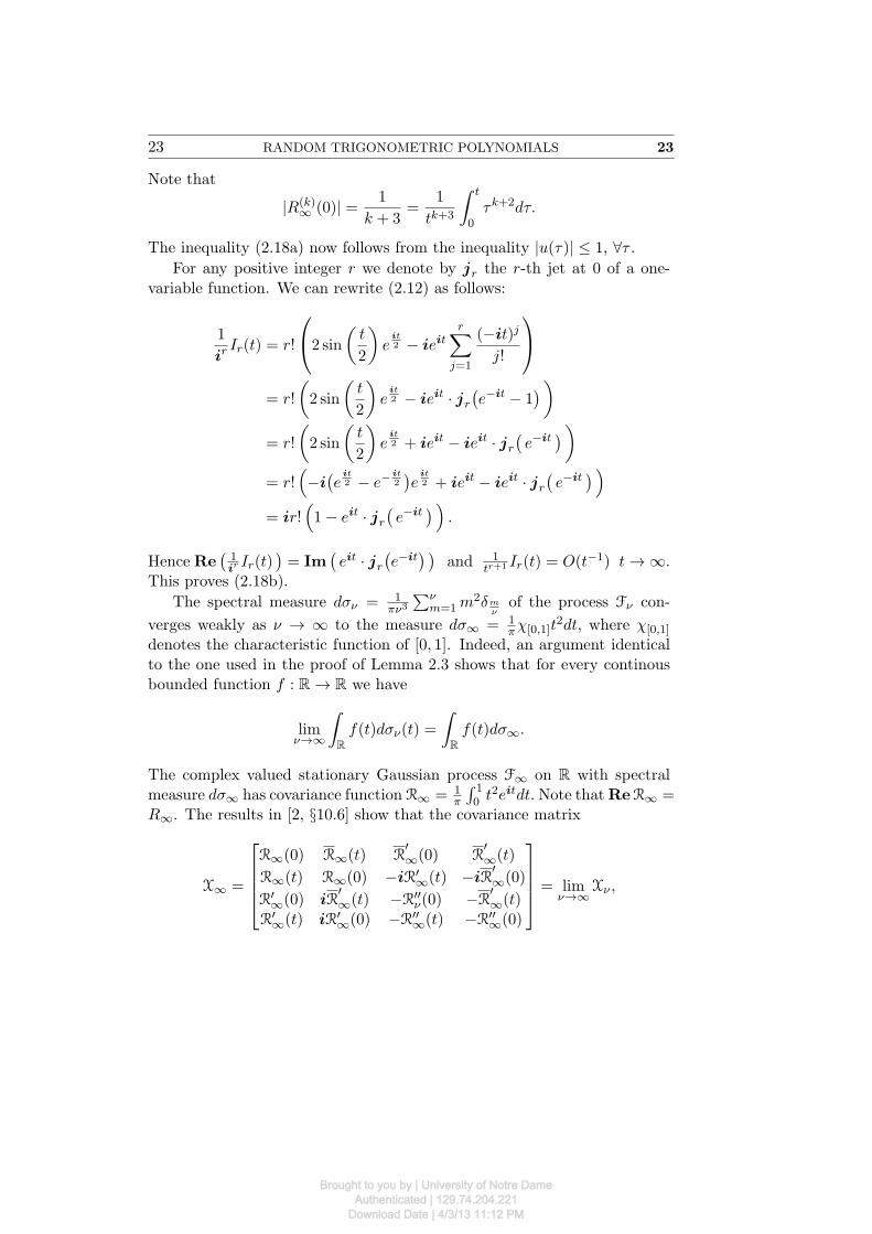
Note that
|R(k)$ (0)| = 1
k + 3=
1
tk+3
& t
0(k+2d(.
The inequality (2.18a) now follows from the inequality |u(()| ! 1, )( .For any positive integer r we denote by jr the r-th jet at 0 of a one-
variable function. We can rewrite (2.12) as follows:
1
irIr(t) = r!
C
D2 sin
"t
2
#e
it2 ' ieit
r!
j=1
('it)j
j!
E
F
= r!
"2 sin
"t
2
#e
it2 ' ieit · jr
'e!it ' 1
(#
= r!
"2 sin
"t
2
#e
it2 + ieit ' ieit · jr
'e!it
(#
= r!+'i'e
it2 ' e!
it2(e
it2 + ieit ' ieit · jr
'e!it
( -
= ir!+1' eit · jr
'e!it
( -.
HenceRe'1ir Ir(t)
(= Im
'eit · jr
'e!it
( (and 1
tr+1 Ir(t) = O(t!1) t $ %.This proves (2.18b).
The spectral measure d/! = 1"!3H!
m=1m2)m
!of the process F! con-
verges weakly as ! $ % to the measure d/$ = 1"1[0,1]t
2dt, where 1[0,1]
denotes the characteristic function of [0, 1]. Indeed, an argument identicalto the one used in the proof of Lemma 2.3 shows that for every continousbounded function f : R $ R we have
lim!#$
&
Rf(t)d/!(t) =
&
Rf(t)d/$.
The complex valued stationary Gaussian process F$ on R with spectralmeasure d/$ has covariance function R$ = 1
"
G 10 t2eitdt.Note thatReR$ =
R$. The results in [2, §10.6] show that the covariance matrix
X$ =
/
0001
R$(0) R$(t) R"$(0) R
"$(t)
R$(t) R$(0) 'iR"$(t) 'iR
"$(0)
R"$(0) iR
"$(t) 'R""
!(0) 'R"$(t)
R"$(t) iR"
$(0) 'R""$(t) 'R""
$(0)
2
3334= lim
!#$X! ,
Brought to you by | University of Notre DameAuthenticated | 129.74.204.221
Download Date | 4/3/13 11:12 PM
24 LIVIU I. NICOLAESCU 24
is nondegenerate. The equality detReX$(t) *= 0, )t # R implies as inRemark 2.2 that µ$(t) *= 0, |*$(t)| < 1, )t # R, where
µ$ =('2
0 'R2$)'2 ' '0(R"
$)2
'20 'R2
$, *$ =
R""$('2
0 'R2$) + (R"
$)2R$('2
0 'R2$)'2 ' '0(R"
$)2.
This proves (2.18c). The equality (2.18d) follows from the Taylor expansionof R$.
REFERENCES
1. Bleher, P.; Di, X. – Correlations between zeros of a random polynomial, J. Statist.Phys., 88 (1997), 269–305.
2. Cramer, H.; Leadbetter, M.R. – Stationary and Related Stochastic Processes.Sample Function Properties and Their Applications, Dover Publications, Inc., Mine-ola, NY, 2004.
3. Dunnage, J.E.A – The number of real zeros of a random trigonometric polynomial,Proc. London Math. Soc., 16 (1966), 53–84.
4. Granville, A.; Wigman, I. – The distribution of zeroes of random trigonometricpolynomials, Amer. J. Math., 133 (2011), 295–357.http://front.math.ucdavis.edu/0809.1848
5. Nicolaescu, L.I. – Critical sets of random smooth functions on compact manifolds,http://www.nd.edu/ lnicolae/CritSetStat.pdf, arXiv: 1101.5990.
6. Qualls, C. – On the number of zeros of a stationary Gaussian random polynomial,J. London Math. Soc., 2 (1970), 216–220.
7. Stanley, R.P. – Enumerative Combinatorics, Volume I, Cambridge Studies in Ad-vanced Mathematics, 49, Cambridge University Press, Cambridge, 1997.
Received: 2.I.2012 Department of Mathematics,University of Notre Dame,
Notre Dame,IN 46556-4618,
[email protected]://www.nd.edu/ lnicolae/
Brought to you by | University of Notre DameAuthenticated | 129.74.204.221
Download Date | 4/3/13 11:12 PM