Numerical approximations of solutions of ordinary ...

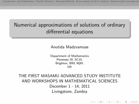
Introduction and Preliminaries Picard’s Theorem One-step Methods Error analysis of the θ- method General explicit one-step method

Numerical approximations of solutions of ordinarydifferential equations

Anotida Madzvamuse

Department of MathematicsPevensey III, 5C15,Brighton, BN1 9QH,

UK

THE FIRST MASAMU ADVANCED STUDY INSTITUTEAND WORKSHOPS IN MATHEMATICAL SCIENCES

December 1 - 14, 2011Livingstone, Zambia


Outline

1 Introduction and Preliminaries

2 Picard’s Theorem

3 One-step Methods

4 Error analysis of the θ- method

5 General explicit one-step method


Applications of ODEs

Ordinary differential equations (ODEs) are a fundamental tool in

Applied mathematics,

mathematical modelling

They can be found in the modelling of

biological systems,

population dynamics,

micro/macroeconomics,

game theory,

financial mathematics.

They also constitute an important branch of mathematics withapplications to different fields such as geometry, mechanics, partialdifferential equations, dynamical systems, mathematical astronomyand physics.


Applications of ODEs

The problem consists of finding y : I −→ R such that it satisfiesthe differential equation

y ′ :=dy

dx= f (x , y(x)) (1)

and the initial condition

y(x0) = y0. (2)

The above is known as an initial value problem (IVP)


The need for computations

Note that an analytical solution of (1)-(2) can be found onlyin very particular situations which are usually quite simpleones.

In general, especially in equations that are of modellingrelevance, there is no systematic way of writing down aformula for the function y(x).

Therefore, in applications where the quantitative knowledge ofthe solution is fundamental one has to turn to a numerical(i.e., digital or computer) approximation of y(x). This is acomputational mathematics problem. There are three mainquestions raised by a computational mathematics problem,such as ours.


Discretisation

The first question is about our ability to come up with acomputable version of the problem. For instance, in (1) thereare derivatives that appear, but on a computer a derivative (oran integral) cannot be evaluated exactly and it needs to bereplaced by some approximation.

Also, there is a continuous infinity of time instants between x0

and x0 + T > x0, it is not possible to determine (not even toapproximate) y(x) for each x ∈ [x0, x0 + T ) and one has tosettle for a finite number of points x0 < x1 < · · · < xN = T .

The process of transforming a continuous problem (whichinvolves continuous infinity of operations) into a finite numberof operations is called discretisation and constitutes the firstphase of establishing a computational method.


Numerical Analysis

The second important question regarding a computationalmethod is to understand whether it yields the wanted results.We want to guarantee that the figures that the computer willoutput are really related to the problem.

It must be checked mathematically that the discrete solution(i.e., the solution of the discretised problem) is a goodapproximation of the problem and deserves the name ofapproximate solution.

This is usually done by conducting an error analysis, whichinvolves concepts such as stability, consistency andconvergence.


Efficiency and implementation

Finally, the third important question regarding acomputational method is that of efficiency and its actualimplementation on a computer. By efficiency, roughlyspeaking, we mean the amount of time that we should bewaiting to compute the solution. It is very easy to write analgorithm that computes a quantity, but it is less easy to writeone that will do it effectively.

Once a discretisation is found to be convergent and to havean acceptable level of efficiency, it can be implemented byusing a computer language, and used for practical purposes.


Deliverables of the lecture series

The main goal of this course is to derive, understand, analyseand implement effective numerical algorithms that provide(good) approximations to the solution y of problem (1)-(2).

A theoretical stream in which we derive and analyse thevarious methods

A practical stream where these methods are coded on acomputer using easy progamming languages such as Matlabor Octave (a free and legal competitor of Matlab with verysimilar syntax) or Scilab (also free and very good qualitysoftware with a Matlab-equivalent syntax).

The implementation of methods is fundamental inunderstanding and appreciating the methods and it provides agood feeling of reward once a numerical method is(successfully) seen in action.


Picard’s theorem

In general, even if f (x , y(x)) is a continuous function, there is noguarantee that the initial value problem (1)-(2) possesses a uniquesolution. Fortunately, under a further mild condition on thefunction f (x , y(x)), the existence and uniqueness of a solution to(1)-(2) can be ensured: the result is encapsulated in the nexttheorem.


Picard’s Theorem I


Picard’s Theorem II

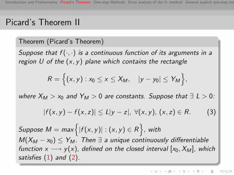
Theorem (Picard’s Theorem)

Suppose that f (·, ·) is a continuous function of its arguments in aregion U of the (x , y) plane which contains the rectangle

R ={

(x , y) : x0 ≤ x ≤ XM , |y − y0| ≤ YM

},

where XM > x0 and YM > 0 are constants. Suppose that ∃ L > 0:

|f (x , y)− f (x , z)| ≤ L|y − z |, ∀(x , y), (x , z) ∈ R. (3)

Suppose M = max{|f (x , y)| : (x , y) ∈ R

}, with

M(XM − x0) ≤ YM . Then ∃ a unique continuously differentiablefunction x −→ y(x), defined on the closed interval [x0,XM ], whichsatisfies (1) and (2).


Picard’s Theorem: Conceptual Proof I

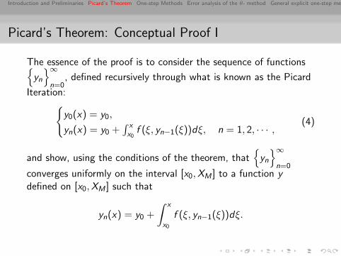
The essence of the proof is to consider the sequence of functions{yn

}∞n=0

, defined recursively through what is known as the Picard

Iteration:{y0(x) = y0,

yn(x) = y0 +∫ xx0

f (ξ, yn−1(ξ))dξ, n = 1, 2, · · · ,(4)

and show, using the conditions of the theorem, that{

yn

}∞n=0

converges uniformly on the interval [x0,XM ] to a function ydefined on [x0,XM ] such that

yn(x) = y0 +

∫ x

x0

f (ξ, yn−1(ξ))dξ.


Picard’s Theorem: Conceptual Proof II

This then implies that y is continuously differentiable on [x0,XM ]and it satisfies the differential equation (1) and the initial condition(2). The uniqueness of the solution follows from the Lipschitzcondition.


Picard’s Theorem: System of ODEs

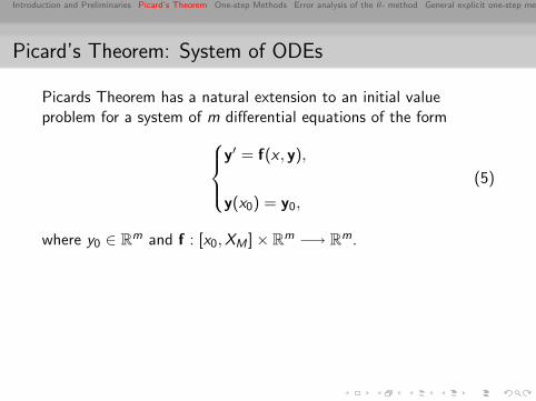
Picards Theorem has a natural extension to an initial valueproblem for a system of m differential equations of the form

y′ = f(x , y),

y(x0) = y0,

(5)

where y0 ∈ Rm and f : [x0,XM ]× Rm −→ Rm.



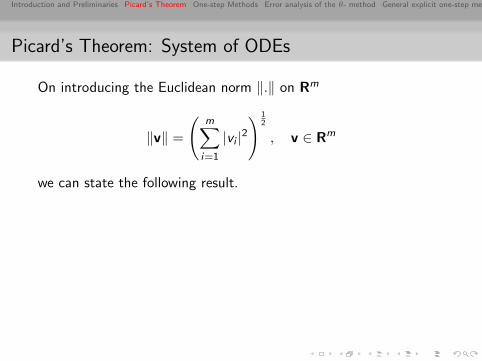
On introducing the Euclidean norm ‖.‖ on Rm

‖v‖ =

(m∑

i=1

|vi |2) 1

2

, v ∈ Rm

we can state the following result.



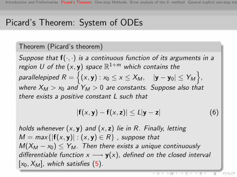
Theorem (Picard’s theorem)

Suppose that f(·, ·) is a continuous function of its arguments in aregion U of the (x , y) space R1+m which contains the

parallelepiped R ={

(x , y) : x0 ≤ x ≤ XM , |y − y0| ≤ YM

},

where XM > x0 and YM > 0 are constants. Suppose also thatthere exists a positive constant L such that

|f(x , y)− f(x , z)| ≤ L|y − z| (6)

holds whenever (x , y) and (x , z) lie in R. Finally, lettingM = max{|f(x , y)| : (x , y) ∈ R} , suppose thatM(XM − x0) ≤ YM . Then there exists a unique continuouslydifferentiable function x −→ y(x), defined on the closed interval[x0,XM ], which satisfies (5).



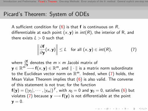
A sufficient condition for (6) is that f is continuous on R,differentiable at each point (x , y) in int(R), the interior of R, andthere exists L > 0 such that∥∥∥∥ ∂f

∂y(x , y)

∥∥∥∥ ≤ L for all (x , y) ∈ int(R), (7)

where ∂f∂y denotes the m ×m Jacobi matrix of

y ∈ Rm −→ f(x , y) ∈ Rm, and ‖ · ‖ is a matrix norm subordinateto the Euclidean vector norm on Rm. Indeed, when (7) holds, theMean Value Theorem implies that (6) is also valid. The converseof this statement is not true; for the functionf(y) = (|y1|, · · · , |ym|)T , with x0 = 0 and y0 = 0, satisfies (6) butviolates (7) because y −→ f(y) is not differentiable at the pointy = 0.



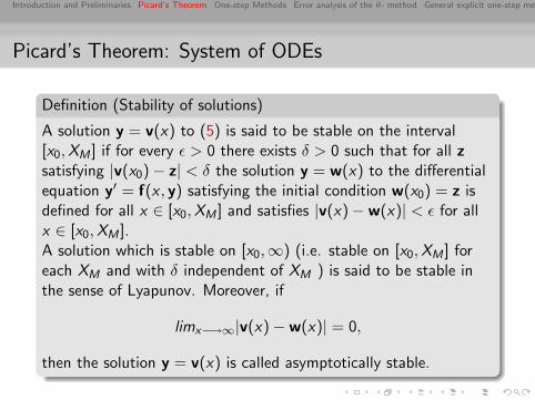
Definition (Stability of solutions)

A solution y = v(x) to (5) is said to be stable on the interval[x0,XM ] if for every ε > 0 there exists δ > 0 such that for all zsatisfying |v(x0)− z| < δ the solution y = w(x) to the differentialequation y′ = f(x , y) satisfying the initial condition w(x0) = z isdefined for all x ∈ [x0,XM ] and satisfies |v(x)−w(x)| < ε for allx ∈ [x0,XM ].A solution which is stable on [x0,∞) (i.e. stable on [x0,XM ] foreach XM and with δ independent of XM ) is said to be stable inthe sense of Lyapunov. Moreover, if

limx−→∞|v(x)−w(x)| = 0,

then the solution y = v(x) is called asymptotically stable.



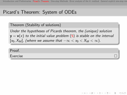
Theorem (Stability of solutions)

Under the hypotheses of Picards theorem, the (unique) solutiony = v(x) to the initial value problem (5) is stable on the interval[x0,XM ], (where we assume that −∞ < x0 < XM < ∞).

Proof.

Exercise


Euler’s method and its relatives: the θ-method

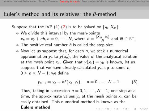
Suppose that the IVP (1)-(2) is to be solved on [x0,XM ].

We divide this interval by the mesh-pointsxn = x0 + nh, n = 0, · · · ,N, where h = (XM−x0)

N and N ∈ Z+.

The positive real number h is called the step size.

Now let us suppose that, for each n, we seek a numericalapproximation yn to y(xn), the value of the analytical solutionat the mesh point xn. Given that y(x0) = y0 is known, let ussuppose that we have already calculated yn, up to some n,0 ≤ n ≤ N − 1; we define

yn+1 = yn + hf (xn, yn), n = 0, · · · ,N − 1. (8)

Thus, taking in succession n = 0, 1, · · · ,N − 1, one step at atime, the approximate values yn at the mesh points xn can beeasily obtained. This numerical method is known as theEulers method.


Euler’s method: Method II

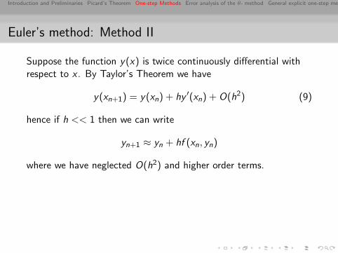
Suppose the function y(x) is twice continuously differential withrespect to x . By Taylor’s Theorem we have

y(xn+1) = y(xn) + hy ′(xn) + O(h2) (9)

hence if h << 1 then we can write

yn+1 ≈ yn + hf (xn, yn)

where we have neglected O(h2) and higher order terms.


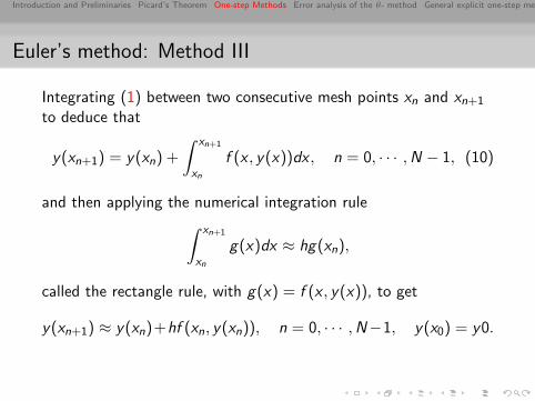
Euler’s method: Method III

Integrating (1) between two consecutive mesh points xn and xn+1

to deduce that

y(xn+1) = y(xn) +

∫ xn+1

xn

f (x , y(x))dx , n = 0, · · · ,N − 1, (10)

and then applying the numerical integration rule∫ xn+1

xn

g(x)dx ≈ hg(xn),

called the rectangle rule, with g(x) = f (x , y(x)), to get

y(xn+1) ≈ y(xn)+hf (xn, y(xn)), n = 0, · · · ,N−1, y(x0) = y0.


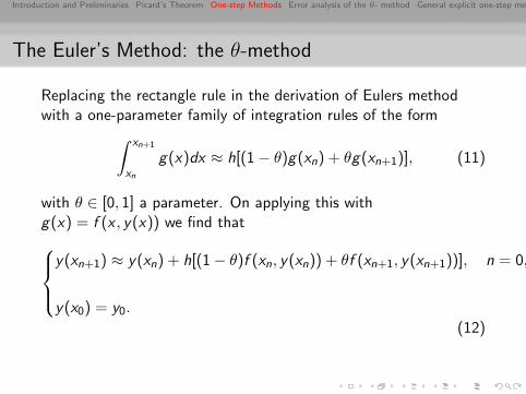
The Euler’s Method: the θ-method

Replacing the rectangle rule in the derivation of Eulers methodwith a one-parameter family of integration rules of the form∫ xn+1

xn

g(x)dx ≈ h[(1− θ)g(xn) + θg(xn+1)], (11)

with θ ∈ [0, 1] a parameter. On applying this withg(x) = f (x , y(x)) we find that

y(xn+1) ≈ y(xn) + h[(1− θ)f (xn, y(xn)) + θf (xn+1, y(xn+1))], n = 0, · · · ,N − 1,

y(x0) = y0.

(12)


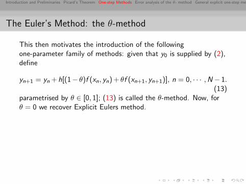
The Euler’s Method: the θ-method

This then motivates the introduction of the followingone-parameter family of methods: given that y0 is supplied by (2),define

yn+1 = yn + h[(1− θ)f (xn, yn)+ θf (xn+1, yn+1)], n = 0, · · · ,N − 1.(13)

parametrised by θ ∈ [0, 1]; (13) is called the θ-method. Now, forθ = 0 we recover Explicit Eulers method.


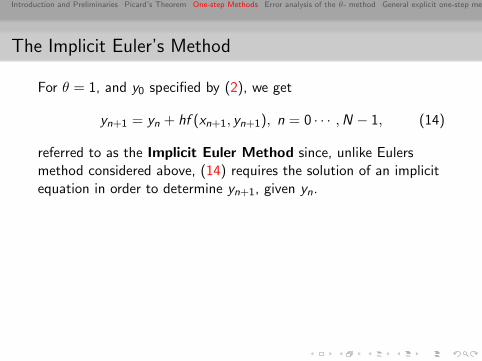
The Implicit Euler’s Method

For θ = 1, and y0 specified by (2), we get

yn+1 = yn + hf (xn+1, yn+1), n = 0 · · · ,N − 1, (14)

referred to as the Implicit Euler Method since, unlike Eulersmethod considered above, (14) requires the solution of an implicitequation in order to determine yn+1, given yn.


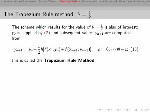
The Trapezium Rule method: θ = 12

The scheme which results for the value of θ = 12 is also of interest:

y0 is supplied by (2) and subsequent values yn+1 are computedfrom

yn+1 = yn +1

2h[f (xn, yn)+ f (xn+1, yn+1)], n = 0, · · ·N−1; (15)

this is called the Trapezium Rule Method.


Example 1

Given the IVPy ′ = x − y2, y(0) = 0,

on the interval of x ∈ [0, 0.4], we compute an approximate solutionusing the θ-method, for θ = 0, θ = 1

2 and θ = 1, using the stepsize h = 0.1. The results are shown in Table 1. In the case of thetwo implicit methods, corresponding to θ = 1

2 and θ = 1, thenonlinear equations have been solved by a fixed-point iteration.For comparison, we also compute the value of the analyticalsolution y(x) at the mesh points xn = 0.1× n, n = 0, · · · , 4. Sincethe solution is not available in closed form, we use a Picarditeration to calculate an accurate approximation to the analyticalsolution on the interval [0, 0.4] and call this the exact solution.


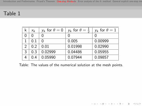
Table 1

k xk yk for θ = 0 yk for θ = 12 yk for θ = 1

0 0 0 0 0

1 0.1 0 0.005 0.00999

2 0.2 0.01 0.01998 0.02990

3 0.3 0.02999 0.04486 0.05955

4 0.4 0.05990 0.07944 0.09857

Table: The values of the numerical solution at the mesh points.


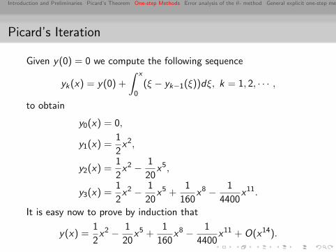
Picard’s Iteration

Given y(0) = 0 we compute the following sequence

yk(x) = y(0) +

∫ x

0(ξ − yk−1(ξ))dξ, k = 1, 2, · · · ,

to obtain

y0(x) = 0,

y1(x) =1

2x2,

y2(x) =1

2x2 − 1

20x5,

y3(x) =1

2x2 − 1

20x5 +

1

160x8 − 1

4400x11.

It is easy now to prove by induction that

y(x) =1

2x2 − 1

20x5 +

1

160x8 − 1

4400x11 + O(x14).


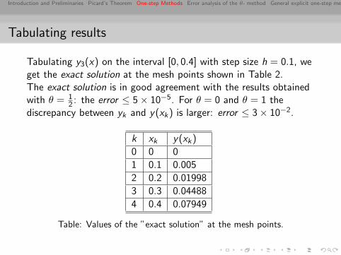
Tabulating results

Tabulating y3(x) on the interval [0, 0.4] with step size h = 0.1, weget the exact solution at the mesh points shown in Table 2.The exact solution is in good agreement with the results obtainedwith θ = 1

2 : the error ≤ 5× 10−5. For θ = 0 and θ = 1 thediscrepancy between yk and y(xk) is larger: error ≤ 3× 10−2.

k xk y(xk)

0 0 0

1 0.1 0.005

2 0.2 0.01998

3 0.3 0.04488

4 0.4 0.07949

Table: Values of the ”exact solution” at the mesh points.


MAPLE: Exact Solution

We note in conclusion that a plot of the analytical solution can beobtained, for example, by using the MAPLE package by typing inthe following at the command line:


First we have to explain what we mean by error.

The exact solution of the initial value problem (1)-(2) is afunction of a continuously varying argument x ∈ [x0,XM ],while the numerical solution yn is only defined at the meshpoints xn, n = 0, · · · ,N, so it is a function of a discreteargument.

We can compare these two functions either by extending insome fashion the approximate solution from the mesh pointsto the whole of the interval [x0,XM ] (say by interpolatingbetween the values yn), or by restricting the function y to themesh points and comparing y(xn) with yn for n = 0, · · · ,N.

Since the first of these approaches is somewhat arbitrarybecause it does not correspond to any procedure performed ina practical computation, we adopt the second approach, andwe define the global error e by

en = y(xn)− yn, n = 0, · · · ,N.


θ = 0

We wish to investigate the decay of the global error for theθ-method with respect to the reduction of the mesh size h.

From the Explicit Euler’s method

yn+1 = yn + hf (xn, yn), n = 0, · · · ,N, y0 given

we can define the Truncation erorr by

Tn =y(xn+1)− y(xn)

h− f (xn, y(xn)), (16)

obtained by inserting the analytical solution y(x) into thenumerical method and dividing by the mesh size.

Indeed, it measures the extent to which the analytical solutionfails to satisfy the difference equation for Eulers method.


θ = 0 Continued

By noting that f (xn, y(xn)) = y ′(xn) and applying TaylorsTheorem, it follows from (16) that there exists ξn ∈ (xn, xn+1)such that

Tn =1

2hy ′′(ξn) (17)

where we have assumed that that f is a sufficiently smoothfunction of two variables so as to ensure that y ′′ exists and isbounded on the interval [x0,XM ]. Since from the definition ofEulers method

0 =yn+1 − yn

h− f (xn, yn),

on subtracting this from (16), we deduce that

en+1 = en + h[f (xn, y(xn))− f (xn, yn)] + hTn.


θ = 0 Continued

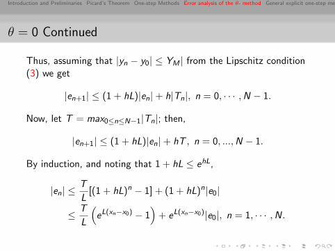
Thus, assuming that |yn − y0| ≤ YM | from the Lipschitz condition(3) we get

|en+1| ≤ (1 + hL)|en|+ h|Tn|, n = 0, · · · ,N − 1.

Now, let T = max0≤n≤N−1|Tn|; then,

|en+1| ≤ (1 + hL)|en|+ hT , n = 0, ...,N − 1.

By induction, and noting that 1 + hL ≤ ehL,

|en| ≤T

L[(1 + hL)n − 1] + (1 + hL)n|e0|

≤ T

L

(eL(xn−x0) − 1

)+ eL(xn−x0)|e0|, n = 1, · · · ,N.


θ = 0 Continued

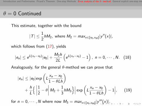
This estimate, together with the bound

|T | ≤ 1

2hM2, where M2 = maxx∈[x0,xM ]|y ′′(x)|,

which follows from (17), yields

|en| ≤ eL(xn−x0)|e0|+M2h

2L

(eL(xn−x0) − 1

), n = 0, · · · ,N. (18)

Analogously, for the general θ-method we can prove that

|en| ≤ |e0|exp(

Lxn − x0

1− θLh

)+

h

L

{ ∣∣∣∣12 − θ

∣∣∣∣M2 +1

3hM3

}∣∣∣ exp(Lxn − x0

1− θLh

)− 1∣∣∣, (19)

for n = 0, · · · ,N where now M3 = maxx∈[x0,xM ]|y ′′′(x)|.


Orders of Convergence

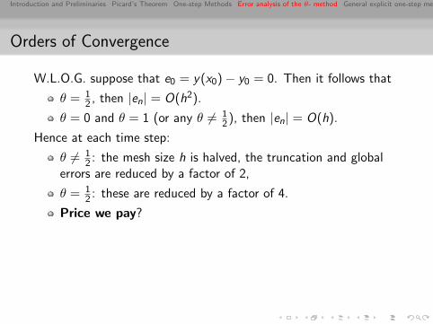
W.L.O.G. suppose that e0 = y(x0)− y0 = 0. Then it follows that

θ = 12 , then |en| = O(h2).

θ = 0 and θ = 1 (or any θ 6= 12), then |en| = O(h).

Hence at each time step:

θ 6= 12 : the mesh size h is halved, the truncation and global

errors are reduced by a factor of 2,

θ = 12 : these are reduced by a factor of 4.

Price we pay?


Improved Explicit Euler’s Method

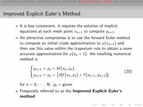
It is less convenient, it requires the solution of implicitequations at each mesh point xn+1 to compute yn+1.

An attractive compromise is to use the forward Euler methodto compute an initial crude approximation to y(xn+1) andthen use this value within the trapezium rule to obtain a moreaccurate approximation for y(xn + 1): the resulting numericalmethod is{

yn+1 = yn + hf (xn, yn),

yn+1 = yn + 12h[f (xn, yn) + f (xn+1, yn+1)],

(20)

for n = 0, · · · ,N, y0 = given.

Frequently referred to as the Improved Explicit Euler’smethod.


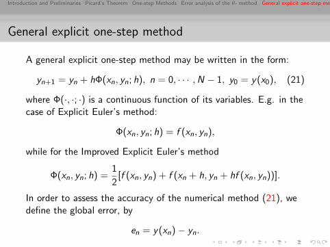
General explicit one-step method

A general explicit one-step method may be written in the form:

yn+1 = yn + hΦ(xn, yn; h), n = 0, · · · ,N − 1, y0 = y(x0), (21)

where Φ(·, ·; ·) is a continuous function of its variables. E.g. in thecase of Explicit Euler’s method:

Φ(xn, yn; h) = f (xn, yn),

while for the Improved Explicit Euler’s method

Φ(xn, yn; h) =1

2[f (xn, yn) + f (xn + h, yn + hf (xn, yn))].

In order to assess the accuracy of the numerical method (21), wedefine the global error, by

en = y(xn)− yn.


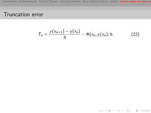
Truncation error

Tn =y(xn+1)− y(xn)

h− Φ(xn, y(xn); h. (22)


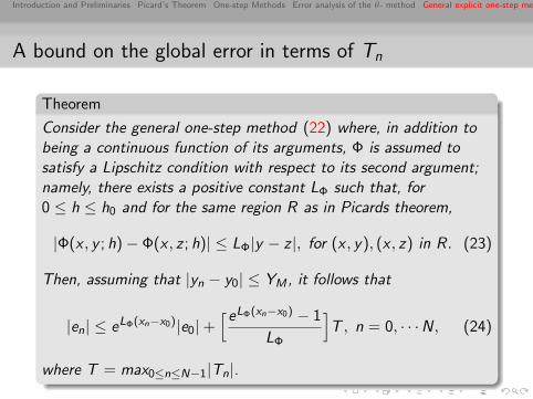
A bound on the global error in terms of Tn

Theorem

Consider the general one-step method (22) where, in addition tobeing a continuous function of its arguments, Φ is assumed tosatisfy a Lipschitz condition with respect to its second argument;namely, there exists a positive constant LΦ such that, for0 ≤ h ≤ h0 and for the same region R as in Picards theorem,

|Φ(x , y ; h)− Φ(x , z ; h)| ≤ LΦ|y − z |, for (x , y), (x , z) in R. (23)

Then, assuming that |yn − y0| ≤ YM , it follows that

|en| ≤ eLΦ(xn−x0)|e0|+[eLΦ(xn−x0) − 1

LΦ

]T , n = 0, · · ·N, (24)

where T = max0≤n≤N−1|Tn|.


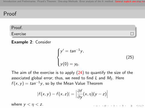
Proof

Proof.

Exercise

Example 2: Consider y ′ = tan−1y ,

y(0) = y0.

(25)

The aim of the exercise is to apply (24) to quantify the size of theassociated global error; thus, we need to find L and M2. Heref (x , y) = tan−1y , so by the Mean Value Theorem

|f (x , y)− f (x , z)| =∣∣∣∂f

∂y(x , η)(y − z)

∣∣∣where y < η < z .


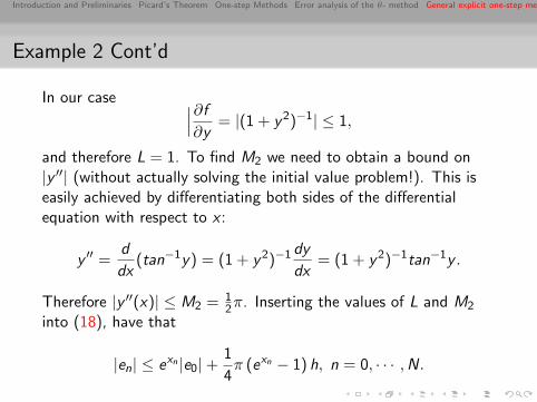
Example 2 Cont’d

In our case ∣∣∣∂f

∂y= |(1 + y2)−1| ≤ 1,

and therefore L = 1. To find M2 we need to obtain a bound on|y ′′| (without actually solving the initial value problem!). This iseasily achieved by differentiating both sides of the differentialequation with respect to x :

y ′′ =d

dx(tan−1y) = (1 + y2)−1 dy

dx= (1 + y2)−1tan−1y .

Therefore |y ′′(x)| ≤ M2 = 12π. Inserting the values of L and M2

into (18), have that

|en| ≤ exn |e0|+1

4π (exn − 1) h, n = 0, · · · ,N.


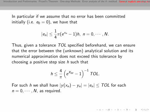
In particular if we assume that no error has been committedinitially (i.e. e0 = 0), we have that

|en| ≤1

4π(exn − 1)h, n = 0, · · · ,N.

Thus, given a tolerance TOL specified beforehand, we can ensurethat the error between the (unknown) analytical solution and itsnumerical approximation does not exceed this tolerance bychoosing a positive step size h such that

h ≤ 4

π

(eXM − 1

)−1TOL.

For such h we shall have |y(xn)− yn| = |en| ≤ TOL for eachn = 0, · · · ,N, as required.


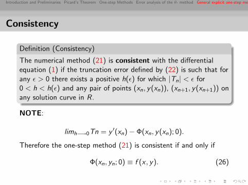
Consistency

Definition (Consistency)

The numerical method (21) is consistent with the differentialequation (1) if the truncation error defined by (22) is such that forany ε > 0 there exists a positive h(ε) for which |Tn| < ε for0 < h < h(ε) and any pair of points (xn, y(xn)), (xn+1, y(xn+1)) onany solution curve in R.

NOTE:

limh−→0Tn = y ′(xn)− Φ(xn, y(xn); 0).

Therefore the one-step method (21) is consistent if and only if

Φ(xn, yn; 0) ≡ f (x , y). (26)


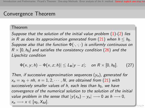
Convergence Theorem

Theorem

Suppose that the solution of the initial value problem (1)-(2) liesin R as does its approximation generated from (21) when h ≤ h0.Suppose also that the function Φ(·, ·; ·) is uniformly continuous onR × [0, h0] and satisfies the consistency condition (26) and theLipschitz condition

Φ(x , y ; h)− Φ(x , z ; h)| ≤ LΦ|y − z |; on R × [0, h0]. (27)

Then, if successive approximation sequences (yn), generated forxn = x0 + nh, n = 1, 2, · · · ,N, are obtained from (21) withsuccessively smaller values of h, each less than h0, we haveconvergence of the numerical solution to the solution of the initialvalue problem in the sense that |y(xn)− yn| −→ 0 as h −→ 0,xn −→ x ∈ [x0,XM ].


Order of accuracy

Definition (Order of accuracy)

The numerical method (21) is said to have order of accuracy p, ifp is the largest positive integer such that, for any sufficientlysmooth solution curve (x , y(x)) in R of the initial value problem(1)-(2), there exist constants K and h0 such that

|Tn| ≤ Khp for 0 < h ≤ h0

for any pair of points (xn, y(xn)), (xn+1, y(xn+1)) on the solutioncurve.

Numerical approximations of solutions of ordinary ...

Documents

Transcript of Numerical approximations of solutions of ordinary ...