PHYSICS OF FLUIDS 26, 072107 (2014)

Flow around a corner in the water impact problemR. Krechetnikova)

Department of Mechanical Engineering, University of California, Santa Barbara, California93106, USA

(Received 28 January 2014; accepted 13 July 2014; published online 30 July 2014)

In this work, we study the local flow in the vicinity of a flat sector of arbitrary angleα in the water impact problem as motivated by recent experimental observations inthe author’s laboratory. The key question is as to why the ejecta formed during theimpact at zero deadrise angle is considerably higher along a straight edge of thesector compared to that near a sharp corner α < π , e.g., if the impacting body is arectangular plate. Resolving this question is made possible by the discovered heremathematical equivalence of the problem to electromagnetic diffraction phenomena.The main result of the present study is the revealed and quantified influence of thegeometry of a flat plate corner on the fluid flow around it, which also contributes tothe understanding of certain three-dimensional effects in the water impact problemand provides a generalization of the classical two-dimensional results on the impactat zero deadrise angle. The offered theoretical solution is also qualitatively supportedwith the help of particle image velocimetry measurements. C© 2014 AIP PublishingLLC. [http://dx.doi.org/10.1063/1.4891229]

I. INTRODUCTION

A. Motivation

Real impact processes are three-dimensional (3D) in nature and, in view of their practicalimportance in various industries and applications (ship building, sea landing, etc.), require accuratemodels providing fundamental insights in the phenomena. Historically, the useful approximate modelof a 3D blunt-body impact onto a free surface of an ideal and incompressible liquid was introducedby Wagner,1 which is based on the flat-disk approximation where the real shape of the impactingbody is substituted in the contact region by a flat disk. While there has been studied a wide varietyof body shapes impacting water, e.g., spheres,2 cones,3 disks,4–6 and wedges,7, 8 to mention a few,in the present work we are interested in the impact of flat-bottomed bodies with sharp corners suchas the rectangular plate in Figure 1 and the local flow structure around such corners—the best wayto think about the general configuration studied here is an impact of a flat sector of angle α at zerodeadrise angle as will be clear from the subsequent discussion, cf. Sec. II A.

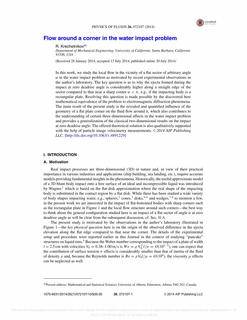
The present study is motivated by the observations in the author’s laboratory illustrated inFigure 1—the key physical question here is on the origin of the observed difference in the ejectaelevation along the flat edge compared to that near the corner. The details of the experimentalsetup and procedure were reported earlier in this Journal in the context of studying “pancake”structures on liquid rims.9 Because the Weber number corresponding to the impact of a plate of widthl = 2.5 cm with velocities V0 = 0.38–1.00 m/s is W e = ρ V 2

0 l/σ = O(102−3), one can expect thatthe contribution of surface tension σ effects is considerably smaller than that of inertia of the fluidof density ρ and, because the Reynolds number is Re = ρV0l/μ = O(104), the viscosity μ effectscan be neglected as well.

a)Present address: Mathematical and Statistical Sciences, University of Alberta, Edmonton, Alberta T6G 2G1, Canada.

1070-6631/2014/26(7)/072107/10/$30.00 C©2014 AIP Publishing LLC26, 072107-1

This article is copyrighted as indicated in the article. Reuse of AIP content is subject to the terms at: http://scitation.aip.org/termsconditions. Downloaded to IP:

76.217.178.83 On: Wed, 30 Jul 2014 15:48:19

072107-2 R. Krechetnikov Phys. Fluids 26, 072107 (2014)

FIG. 1. Impact of a finite-size rectangular plate of dimensions 2lx × 2lz = 2.5 cm × 7.5 cm in the (x, z)-plane on water atspeed 1 m/s and temperature 20 ◦C; perspective view showing the variation of the ejecta elevation along the flat edge andaround the corner 2.5 ms after the impact. The observed behavior persists over the entire range of tested impact velocities,V0 = 0.38–1.00 m/s.

B. Problem statement

As is well-known,10 if there are no mass impulsive forces, then neither convective nor viscousterms can balance the dominant time-derivative term, ∂v/∂t , in the Navier-Stokes equations, butonly the pressure gradients can handle this sudden change in the fluid motion:

∂v∂t

= − 1

ρ∇ p. (1)

Then the incompressibility condition, ∇ · v = 0, implies that the pressure p is a harmonic function,�p = 0, which allows decoupling of the pressure and velocity fields at early times after the impact.As classically argued,10 if the fluid is at rest before the impact, its motion right after the impact ispotential with the velocity potential φ defined such that v = ∇φ. Therefore, adopting the coordinatesystem in Figure 1 brings us to the following formulation of the 3D impact problem of the plateoccupying the region (x, z) ∈ [ − lx, lx; −lz, lz] ≡ with the appropriate boundary conditions:

�φ = 0, x, z ∈ R, y ∈ R−, (2a)

y = 0 :∂φ

∂y= −V0, (x, z) ∈ , (2b)

φ = 0, (x, z) /∈ , (2c)

y = −∞ : |φ| < ∞, (2d)

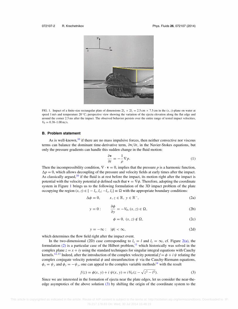
which determines the flow field right after the impact event.In the two-dimensional (2D) case corresponding to lx = l and lz = ∞, cf. Figure 2(a), the

formulation (2) is a particular case of the Hilbert problem,11 which historically was solved in thecomplex plane z = x + iy using the standard techniques for singular integral equations with Cauchykernels.12, 13 Indeed, after the introduction of the complex velocity potential f = φ + i ψ relating thecomplex conjugate velocity potential φ and streamfunction ψ via the Cauchy-Riemann equations,φx = ψy and φy = −ψx, one can appeal to the complex variable methods14 with the result

f (z) = φ(x, y) + i ψ(x, y) = iV0 (z −√

z2 − l2). (3)

Since we are interested in the formation of ejecta near the plate edges, let us consider the near-the-edge asymptotics of the above solution (3) by shifting the origin of the coordinate system to the

This article is copyrighted as indicated in the article. Reuse of AIP content is subject to the terms at: http://scitation.aip.org/termsconditions. Downloaded to IP:

76.217.178.83 On: Wed, 30 Jul 2014 15:48:19

072107-3 R. Krechetnikov Phys. Fluids 26, 072107 (2014)

FIG. 2. 2D impact problem treated in the complex plane, z = x + iy: (a) global problem, (b) near-the-edge region, (c)streamlines in the near-the-edge region computed based on Eq. (3).

edge, z → z′ + l, cf. Figure 2(b). Retaining the leading order non-constant term only we get

f (z′) −iα√

2 z′, (4)

where α = V0

√l with dim α = L3/2T−1. Note that in this approximation the normal velocity vanishes

at the plate surface, v = 0, because we retain the leading order terms only when arriving at (4), whilethe next lower order non-constant term iV0z′ is responsible for satisfying the boundary condition(2b). Expressing z′ in polar coordinates z′ = r eiθ and separating real and imaginary parts of thecomplex velocity potential (4), we get the dimensional velocity potential function

φ = α√

2 r sinθ

2, (5)

which clearly shows the singularity of the velocity field v = ∇φ ∼ r−1/2 near the plate edge. Theintuition behind this solution and thus the origin of ejecta is simple: once the plate impacts thesurface, a layer of displaced liquid beneath it—a wall jet—moves radially and since it fails toaccelerate the bulk of the surrounding liquid, this layer is deflected upwards and forms an ejecta, cf.Figure 2(c) plotted based on Eq. (3). The key mathematical question of this paper is to understandthe dependence of the singularity exponent ν(α) on the sector angle α in 3D case, cf. Figure 3(a):

φ ∼ r ν(α). (6)

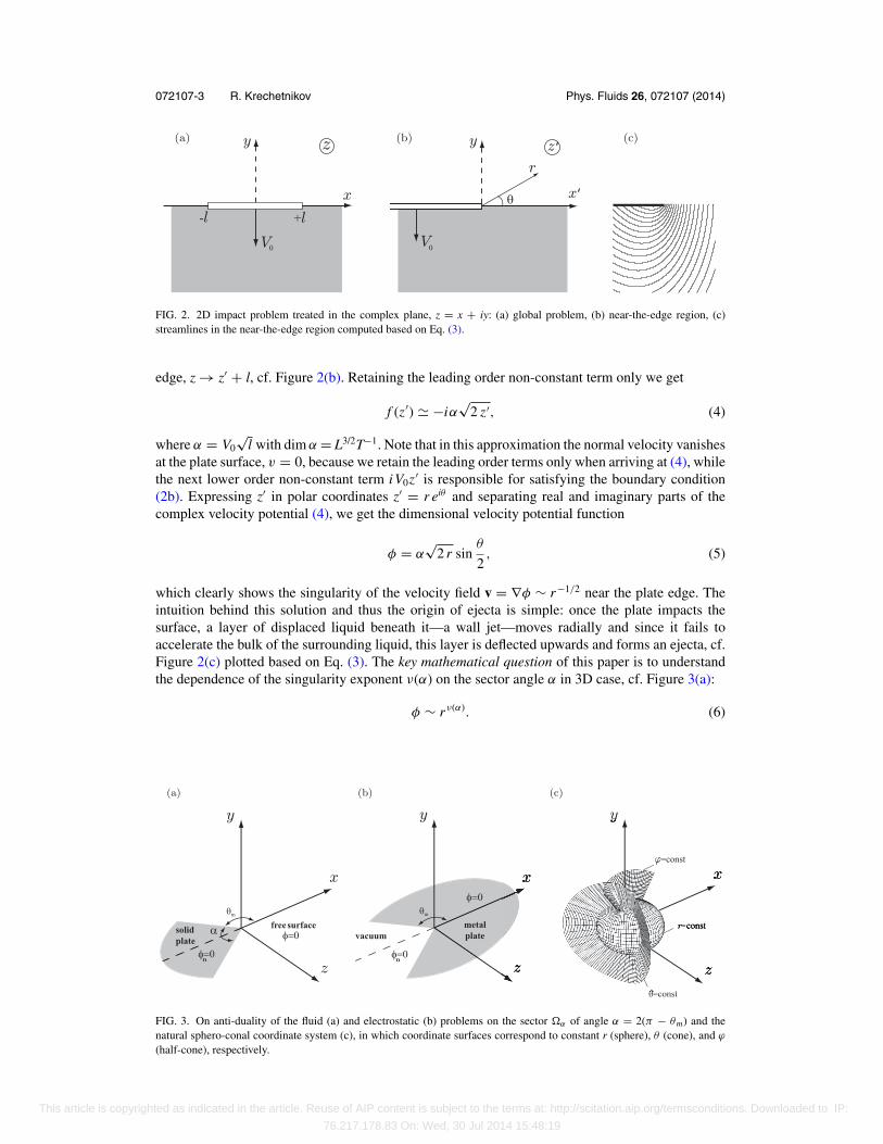
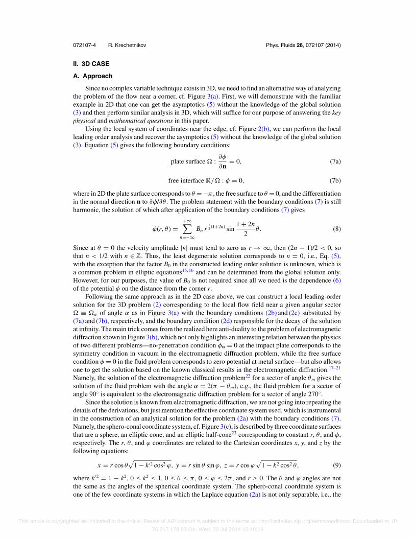
FIG. 3. On anti-duality of the fluid (a) and electrostatic (b) problems on the sector α of angle α = 2(π − θm) and thenatural sphero-conal coordinate system (c), in which coordinate surfaces correspond to constant r (sphere), θ (cone), and ϕ

(half-cone), respectively.

This article is copyrighted as indicated in the article. Reuse of AIP content is subject to the terms at: http://scitation.aip.org/termsconditions. Downloaded to IP:

76.217.178.83 On: Wed, 30 Jul 2014 15:48:19

072107-4 R. Krechetnikov Phys. Fluids 26, 072107 (2014)

II. 3D CASE

A. Approach

Since no complex variable technique exists in 3D, we need to find an alternative way of analyzingthe problem of the flow near a corner, cf. Figure 3(a). First, we will demonstrate with the familiarexample in 2D that one can get the asymptotics (5) without the knowledge of the global solution(3) and then perform similar analysis in 3D, which will suffice for our purpose of answering the keyphysical and mathematical questions in this paper.

Using the local system of coordinates near the edge, cf. Figure 2(b), we can perform the localleading order analysis and recover the asymptotics (5) without the knowledge of the global solution(3). Equation (5) gives the following boundary conditions:

plate surface :∂φ

∂n= 0, (7a)

free interface R/ : φ = 0, (7b)

where in 2D the plate surface corresponds to θ = −π , the free surface to θ = 0, and the differentiationin the normal direction n to ∂φ/∂θ . The problem statement with the boundary conditions (7) is stillharmonic, the solution of which after application of the boundary conditions (7) gives

φ(r, θ ) =+∞∑

n=−∞Bn r

12 (1+2n) sin

1 + 2n

2θ. (8)

Since at θ = 0 the velocity amplitude |v| must tend to zero as r → ∞, then (2n − 1)/2 < 0, sothat n < 1/2 with n ∈ Z. Thus, the least degenerate solution corresponds to n = 0, i.e., Eq. (5),with the exception that the factor B0 in the constructed leading order solution is unknown, which isa common problem in elliptic equations15, 16 and can be determined from the global solution only.However, for our purposes, the value of B0 is not required since all we need is the dependence (6)of the potential φ on the distance from the corner r.

Following the same approach as in the 2D case above, we can construct a local leading-ordersolution for the 3D problem (2) corresponding to the local flow field near a given angular sector ≡ α of angle α as in Figure 3(a) with the boundary conditions (2b) and (2c) substituted by(7a) and (7b), respectively, and the boundary condition (2d) responsible for the decay of the solutionat infinity. The main trick comes from the realized here anti-duality to the problem of electromagneticdiffraction shown in Figure 3(b), which not only highlights an interesting relation between the physicsof two different problems—no-penetration condition φn = 0 at the impact plate corresponds to thesymmetry condition in vacuum in the electromagnetic diffraction problem, while the free surfacecondition φ = 0 in the fluid problem corresponds to zero potential at metal surface—but also allowsone to get the solution based on the known classical results in the electromagnetic diffraction.17–21

Namely, the solution of the electromagnetic diffraction problem22 for a sector of angle θm gives thesolution of the fluid problem with the angle α = 2(π − θm), e.g., the fluid problem for a sector ofangle 90◦ is equivalent to the electromagnetic diffraction problem for a sector of angle 270◦.

Since the solution is known from electromagnetic diffraction, we are not going into repeating thedetails of the derivations, but just mention the effective coordinate system used, which is instrumentalin the construction of an analytical solution for the problem (2a) with the boundary conditions (7).Namely, the sphero-conal coordinate system, cf. Figure 3(c), is described by three coordinate surfacesthat are a sphere, an elliptic cone, and an elliptic half-cone23 corresponding to constant r, θ , and φ,respectively. The r, θ , and ϕ coordinates are related to the Cartesian coordinates x, y, and z by thefollowing equations:

x = r cos θ√

1 − k ′2 cos2 ϕ, y = r sin θ sin ϕ, z = r cos ϕ√

1 − k2 cos2 θ, (9)

where k′2 = 1 − k2, 0 ≤ k2 ≤ 1, 0 ≤ θ ≤ π , 0 ≤ ϕ ≤ 2π , and r ≥ 0. The θ and ϕ angles are notthe same as the angles of the spherical coordinate system. The sphero-conal coordinate system isone of the few coordinate systems in which the Laplace equation (2a) is not only separable, i.e., the

This article is copyrighted as indicated in the article. Reuse of AIP content is subject to the terms at: http://scitation.aip.org/termsconditions. Downloaded to IP:

76.217.178.83 On: Wed, 30 Jul 2014 15:48:19

072107-5 R. Krechetnikov Phys. Fluids 26, 072107 (2014)

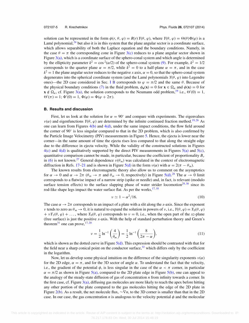
solution can be represented in the form φ(r, θ , ϕ) = R(r) Y(θ , ϕ), where Y(θ , ϕ) = �(θ )�(ϕ) is aLame polynomial,24 but also it is in this system that the plane angular sector is a coordinate surface,which allows separability of both the Laplace equation and the boundary conditions. Namely, inthe case θ = π the corresponding cone in Figure 3(c) reduces to a plane angular sector shown inFigure 3(a), which is a coordinate surface of the sphero-conal system and which angle is determinedby the ellipticity parameter k2 = cos 2(α/2) of the sphero-conal system (9). For example, k2 = 1/2corresponds to the quarter plane α = π /2, while k2 = 0 to a half-plane α = π , and in the casek2 = 1 the plane angular sector reduces to the negative x axis, α = 0, so that the sphero-conal systemdegenerates into the spherical coordinate system (and the Lame polynomials Y(θ , ϕ) into Legendreones)—the 2D case considered in Sec. I B corresponds to ϕ = π /2 and the same θ . Because ofthe physical boundary conditions (7) in the fluid problem, φn(x) = 0 for x ∈ α and φ(x) = 0 forx /∈ α , cf. Figure 3(a), the solution corresponds to the Neumann odd problem,19 i.e., �′(0) = 1,�′(π ) = 1; �′(0) = 1, �(ϕ) = �(ϕ + 2π ).

B. Results and discussion

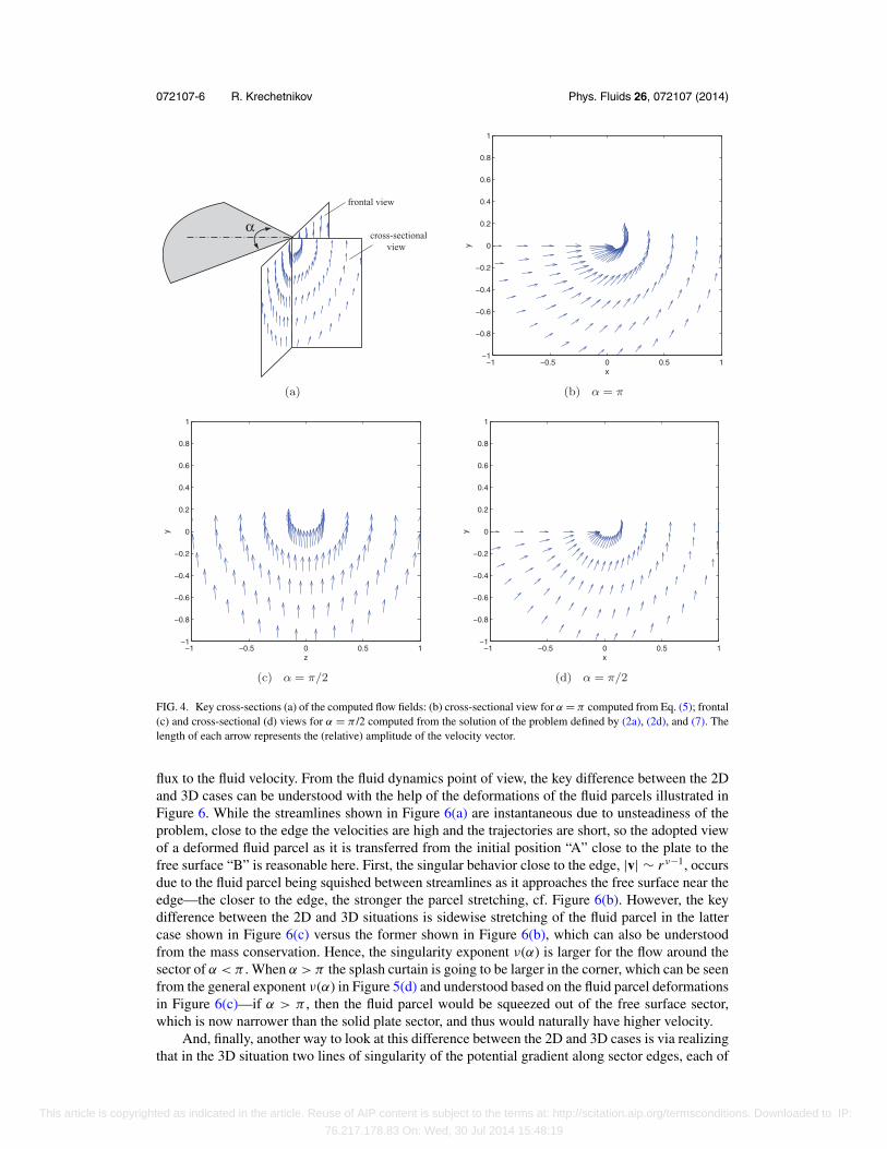
First, let us look at the solution for α = 90◦ and compare with experiments. The eigenvaluesν(α) and eigenfunctions Y(θ , ϕ) are determined by the infinite continued fraction method.19, 26 Asone can learn from Figures 4(b) and 4(d), under the same impact conditions, the flow field aroundthe corner of 90◦ is less singular compared to that in the 2D problem, which is also confirmed bythe Particle Image Velocimetry (PIV) measurements in Figure 5. Hence, the ejecta is lower near thecorner—in the same amount of time the ejecta rises less compared to that along the straight edgedue to the difference in ejecta velocity. While the validity of the constructed solutions in Figures4(c) and 4(d) is qualitatively supported by the direct PIV measurements in Figures 5(a) and 5(c),quantitative comparison cannot be made, in particular, because the coefficient of proportionality Bν

in (6) is not known.27 General dependence ν(θm) was calculated in the context of electromagneticdiffraction in Refs. 17–21 and is shown in Figure 5(d) in the form ν(α) with α = 2(π − θm).

The known results from elecromagnetic theory also allow us to comment on the asymptoticsfor α → 0 and α → 2π (θm → π and θm → 0, respectively) in Figure 5(d).28 The α → 0 limitcorresponds to a flatwise impact of a narrow strip (spike or needle) and, in fact, is relevant (modulosurface tension effects) to the surface slapping phase of water strider locomotion29, 30 since itsrod-like shape legs impact the water surface flat. As per the works,17, 18

ν 1 − α2/16. (10)

The case α → 2π corresponds to an impact of a plate with a slit along the x-axis. Since the exponentν tends to zero as θm → 0, it is natural to expand the solution in powers of ν, i.e., Y(θ , ϕ) = Y0(θ , ϕ)+ νY1(θ , ϕ) + . . . , where Y0(θ , ϕ) corresponds to ν = 0, i.e., when the open part of the xz-plane(free surface) is just the positive x-axis. With the help of standard perturbation theory and Green’stheorem31 one can prove,17, 20

ν = 1

2ln−1

(4

θm

)= 1

2ln−1

(8

2π − α

), (11)

which is shown as the dotted curve in Figure 5(d). This expression should be contrasted with that forthe field near a sharp conical point on the conductor surface,32 which differs only by the coefficientin the logarithm.

Now, let us develop some physical intuition on the difference of the singularity exponents ν(α)for the 2D edge, α = π , and for the 3D sector of angle α. To understand the fact that the velocity,i.e., the gradient of the potential φ, is less singular in the case of the α < π corner, in particularα = π /2 as shown in Figure 5(a), compared to the 2D plate edge in Figure 5(b), one can appeal tothe analogy of the steady-state diffusion of gas of concentration n from infinity towards a corner. Inthe first case, cf. Figure 3(a), diffusing gas molecules are more likely to reach the apex before hittingany other portion of the plate compared to the gas molecules hitting the edge of the 2D plate inFigure 2(b). As a result, the net molecule flux, ∼∇n, to the 3D corner is smaller than that in the 2Dcase. In our case, the gas concentration n is analogous to the velocity potential φ and the molecular

This article is copyrighted as indicated in the article. Reuse of AIP content is subject to the terms at: http://scitation.aip.org/termsconditions. Downloaded to IP:

76.217.178.83 On: Wed, 30 Jul 2014 15:48:19

072107-6 R. Krechetnikov Phys. Fluids 26, 072107 (2014)

frontal view

cross-sectional view

α

(a)

−1 −0.5 0 0.5 1−1

−0.8

−0.6

−0.4

−0.2

0

0.2

0.4

0.6

0.8

1

x

y

(b) α = π

−1 −0.5 0 0.5 1−1

−0.8

−0.6

−0.4

−0.2

0

0.2

0.4

0.6

0.8

1

z

y

(c) α = π/2

−1 −0.5 0 0.5 1−1

−0.8

−0.6

−0.4

−0.2

0

0.2

0.4

0.6

0.8

1

x

y

(d) α = π/2

FIG. 4. Key cross-sections (a) of the computed flow fields: (b) cross-sectional view for α = π computed from Eq. (5); frontal(c) and cross-sectional (d) views for α = π /2 computed from the solution of the problem defined by (2a), (2d), and (7). Thelength of each arrow represents the (relative) amplitude of the velocity vector.

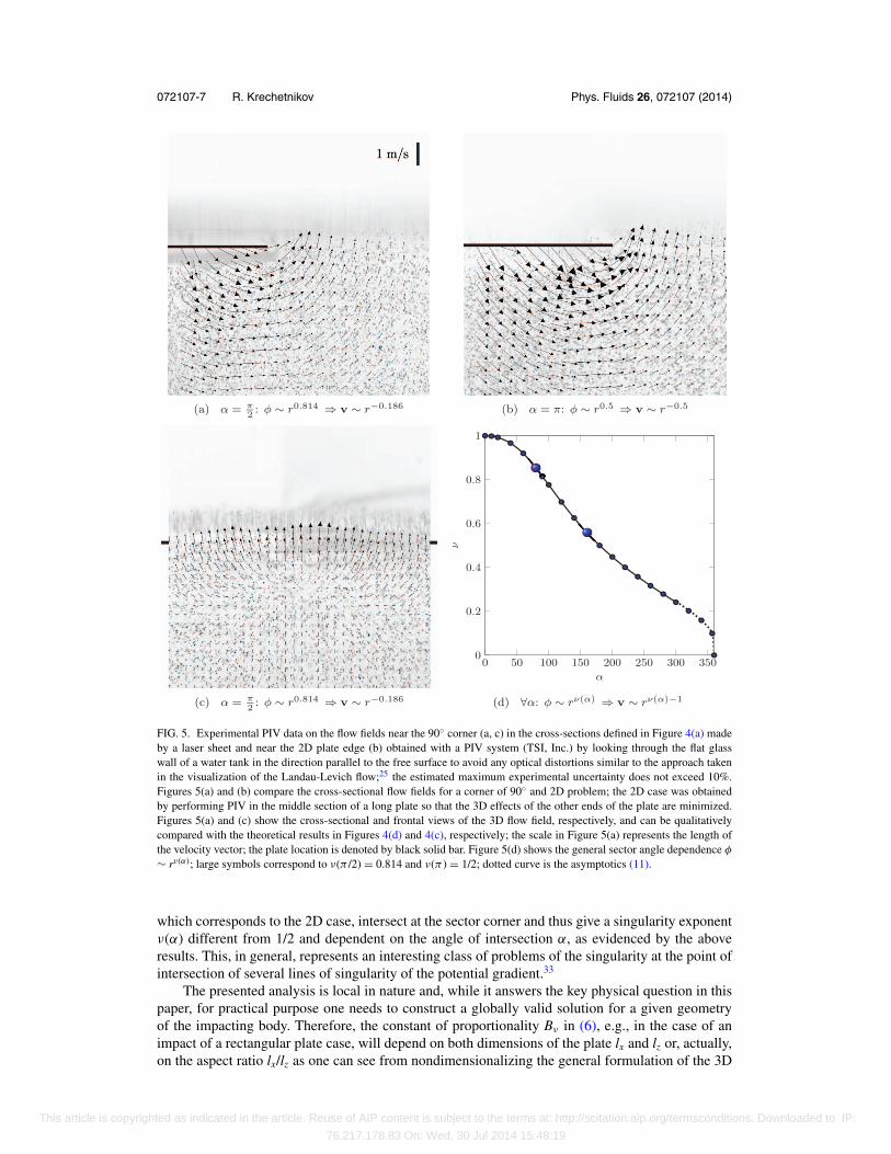
flux to the fluid velocity. From the fluid dynamics point of view, the key difference between the 2Dand 3D cases can be understood with the help of the deformations of the fluid parcels illustrated inFigure 6. While the streamlines shown in Figure 6(a) are instantaneous due to unsteadiness of theproblem, close to the edge the velocities are high and the trajectories are short, so the adopted viewof a deformed fluid parcel as it is transferred from the initial position “A” close to the plate to thefree surface “B” is reasonable here. First, the singular behavior close to the edge, |v| ∼ r ν−1, occursdue to the fluid parcel being squished between streamlines as it approaches the free surface near theedge—the closer to the edge, the stronger the parcel stretching, cf. Figure 6(b). However, the keydifference between the 2D and 3D situations is sidewise stretching of the fluid parcel in the lattercase shown in Figure 6(c) versus the former shown in Figure 6(b), which can also be understoodfrom the mass conservation. Hence, the singularity exponent ν(α) is larger for the flow around thesector of α < π . When α > π the splash curtain is going to be larger in the corner, which can be seenfrom the general exponent ν(α) in Figure 5(d) and understood based on the fluid parcel deformationsin Figure 6(c)—if α > π , then the fluid parcel would be squeezed out of the free surface sector,which is now narrower than the solid plate sector, and thus would naturally have higher velocity.

And, finally, another way to look at this difference between the 2D and 3D cases is via realizingthat in the 3D situation two lines of singularity of the potential gradient along sector edges, each of

This article is copyrighted as indicated in the article. Reuse of AIP content is subject to the terms at: http://scitation.aip.org/termsconditions. Downloaded to IP:

76.217.178.83 On: Wed, 30 Jul 2014 15:48:19

072107-7 R. Krechetnikov Phys. Fluids 26, 072107 (2014)

FIG. 5. Experimental PIV data on the flow fields near the 90◦ corner (a, c) in the cross-sections defined in Figure 4(a) madeby a laser sheet and near the 2D plate edge (b) obtained with a PIV system (TSI, Inc.) by looking through the flat glasswall of a water tank in the direction parallel to the free surface to avoid any optical distortions similar to the approach takenin the visualization of the Landau-Levich flow;25 the estimated maximum experimental uncertainty does not exceed 10%.Figures 5(a) and (b) compare the cross-sectional flow fields for a corner of 90◦ and 2D problem; the 2D case was obtainedby performing PIV in the middle section of a long plate so that the 3D effects of the other ends of the plate are minimized.Figures 5(a) and (c) show the cross-sectional and frontal views of the 3D flow field, respectively, and can be qualitativelycompared with the theoretical results in Figures 4(d) and 4(c), respectively; the scale in Figure 5(a) represents the length ofthe velocity vector; the plate location is denoted by black solid bar. Figure 5(d) shows the general sector angle dependence φ

∼ rν(α); large symbols correspond to ν(π /2) = 0.814 and ν(π ) = 1/2; dotted curve is the asymptotics (11).

which corresponds to the 2D case, intersect at the sector corner and thus give a singularity exponentν(α) different from 1/2 and dependent on the angle of intersection α, as evidenced by the aboveresults. This, in general, represents an interesting class of problems of the singularity at the point ofintersection of several lines of singularity of the potential gradient.33

The presented analysis is local in nature and, while it answers the key physical question in thispaper, for practical purpose one needs to construct a globally valid solution for a given geometryof the impacting body. Therefore, the constant of proportionality Bν in (6), e.g., in the case of animpact of a rectangular plate case, will depend on both dimensions of the plate lx and lz or, actually,on the aspect ratio lx/lz as one can see from nondimensionalizing the general formulation of the 3D

This article is copyrighted as indicated in the article. Reuse of AIP content is subject to the terms at: http://scitation.aip.org/termsconditions. Downloaded to IP:

76.217.178.83 On: Wed, 30 Jul 2014 15:48:19

072107-8 R. Krechetnikov Phys. Fluids 26, 072107 (2014)

(a)

AB (b)

A

B (c)

A

B

α

FIG. 6. Deformation of a fluid parcel (shaded) in the near-the-edge region shown in the cross-section (a) as it travels fromunderneath the plate to the free surface along dashed lines in (b,c): 2D (b) vs. 3D (c) case as viewed from the top. Fluid parcelin the 3D case (c) is being stretched sidewise (arrows) for α < π and squished for α > π as opposed to the 2D case (b).

problem (2). While in 2D the solution can be constructed with the dual integral method,34–37 the3D problem is intractable with current analytical methods (2) and would require development of thesolution methods for higher dimensional dual integral equations (these can be obtained by applyingFourier transform in both x and z directions—application of the Fourier transform in this case isjustified by the fact that the singularity of the velocity potential φ is not stronger than that in the 2Dcase). The resulting knowledge of an analytical solution for (2) would allow one to determine theproportionality constant Bν in (6) as a function of lx/lz. Such a solution, however, was constructedexperimentally for some particular impact situations in the context of determining added masses forrectangular plates of a few aspect ratios38, 39 as well as theoretically using singularity theory,40, 41

though the theoretical solutions reduce to series with coefficients determined numerically—in anycase, there is no analytical formula for the dependence Bν(lx/lz). Since the focus of the latter workswas the calculation of added mass, no information on the velocity potential is given to determine thecoefficient Bν(lx/lz). However, as it was shown in the 2D case above, for the purpose of answeringthe key question of this paper we do not need to know the value of the coefficient Bν since all werequire is the dependence (6) of the potential φ on the distance from the corner r.

III. CONCLUSIONS

As inspired by recent experimental observations,9 the present work discusses one of the effectsof three dimensionality of the impacting body, namely, that of the corner of a sector of angleα, on the local flow structure and thus the ejecta evolution in the water impact problem, whichcomplements the existing studies of 3D water impacts. The main finding of this study is the revealedand quantified influence of the geometry of a flat plate corner on the ejecta properties, whichprovides a generalization of the classical 2D results.14 Transparent physical interpretation of theobserved behavior is also offered. While the problems of interest here involve sharp corners, itis worth noting that the development of higher-dimensional Joukowsky transformations based onClifford analysis42, 43 may be a promising tool for solving impact problems if the impacting bodiesdo not have sharp corners. The presented problem motivated by a concrete physical phenomenon, infact, belongs to a wide class of problems in domains with point singularities,44, 45 which deals withestimates for solutions in different function spaces, regularity assertions, solvability of the boundaryvalue problems, and asymptotic formulas for the solutions near singular points. Due to its analogyto other physical phenomena (Sec. II B), one can use the variation of the ejecta elevation near thecorner exemplified in Figure 1 as an illustration of singular behavior in other physical systems wheresuch a direct visual appeal is not possible, e.g., in electromagnetism.

While the mathematical analogy, which helped to solve the problem here, was establishedwith the electromagnetic diffraction theory, one should mention that historically the mathematicalproblem was first analyzed in the context of contact problems in elasticity46–48 with the foundationalcontribution by Galin.46 It is a historical irony that Galin also studied the water impact problem,49 butthe found here mathematical analogy between these problems was not realized then. The problemstudied in the present work is also mathematically equivalent to the potential (aerodynamic) flow

This article is copyrighted as indicated in the article. Reuse of AIP content is subject to the terms at: http://scitation.aip.org/termsconditions. Downloaded to IP:

76.217.178.83 On: Wed, 30 Jul 2014 15:48:19

072107-9 R. Krechetnikov Phys. Fluids 26, 072107 (2014)

around the apex of a plane delta wing50, 51 as well as to wave scattering near the tip of a sector (cornerof a screen) analyzed later by many authors.52, 53

ACKNOWLEDGMENTS

The author is grateful to Dr. Denis Labutin and Dr. Andrei Zelnikov for stimulating discussions,and to Hans Mayer for the help with acquiring the PIV data. This work was partially supportedby the National Science Foundation (NSF) CAREER award under Grant No. 1054267, AmericanChemical Society (ACS) Petroleum Research Fund under Grant No. 51307-ND5, and the NaturalSciences and Engineering Research Council of Canada (NSERC) under Grant No. 6186.

1 H. Wagner, “Uber Stoss- und Gleitvorgange an der Oberflache von Flussigkeiten,” Z. angew. Math. Mech. 12, 193–215(1932).

2 E. G. Richardson, “The impact of a solid on a liquid surface,” Proc. Phys. Soc., London 61, 352–367 (1948).3 M. Schiffman and D. C. Spencer, “The force of impact on a cone striking a water surface (vertical entry),” Commun. Pure

Appl. Math. 4, 379–417 (1951).4 J. W. Glasheen and T. A. McMahon, “Vertical water entry of disks at low Froude numbers,” Phys. Fluids 8, 2078–2083

(1996).5 S. Gaudet, “Numerical simulation of circular disks entering the free surface of a fluid,” Phys. Fluids 10, 2489–2499 (1998).6 E. V. Ermanyuk and M. Ohkusu, “Impact of a disk on shallow water,” J. Fluids Struct. 20, 345–357 (2005).7 T. H. von Karman, “The impact on seaplane floats during landing,” Tech. Rep. 321 (NACA, 1929).8 P. R. Garabedian, “Oblique water entry of a wedge,” Commun. Pure Appl. Math. 6, 157–165 (1953).9 H. C. Mayer and R. Krechetnikov, “Singular structures on liquid rims,” Phys. Fluids 26, 032109 (2014).

10 G. K. Batchelor, An Introduction to Fluid Dynamics (Cambridge University Press, Cambridge, 1967).11 S. G. Mikhlin, Integral Equations (Pergamon Press, New York, 1964).12 F. D. Gakhov, Boundary Value Problems (Pergamon Press, New York, 1966).13 A. D. Polyanin and A. V. Manzhirov, Handbook of Integral Equations (Chapman and Hall/CRC, Boca Raton, FL, 2008).14 M. A. Lavrentiev and B. V. Schabat, Methoden der komplexen Funktionentheorie (Deutscher Verlag der Wissenschaften,

Berlin, 1967).15 M. van Dyke, Perturbation Methods in Fluid Mechanics (Parabolic Press, Stanford, CA, 1975).16 Undetermined factors are a common problem for elliptic equations,15 for which coordinate expansions give only qualitative

results—due to dependence on all boundary conditions local solutions such as the potential flow solution (8) depend onboundary conditions at large distances. Therefore, the determined expansions contain unknown constants, which cannotbe found as they depend on the boundary conditions far from the region of applicability of the constructed solution.

17 B. Noble, “The potential and charge distribution near the tip of a flat angular sector,” Tech. Rep. EM-135 (New YorkUniversity, 1959).

18 J. A. Morrison and J. A. Lewis, “Charge singularity at the corner of a flat plate,” SIAM J. Appl. Math. 31, 233–250 (1976).19 R. Satterwhite and R. G. Kouyoumjian, “Electromagnetic diffraction by a perfectly-conducting plane-angular sector,”

Tech. Rep. 2183-2 (ElectroSci. Lab., Ohio State University, Columbus, OH, 1970).20 R. de Smedt, “Electric singularity near the tip of a sharp cone,” IEEE Trans. Antennas Propag. 36, 152–155 (1988).21 R. de Smedt and J. G. van Bladel, “Field singularities at the tip of a metallic cone of arbitrary cross-section,” IEEE Trans.

Antennas Propag. 34, 865–870 (1986).22 Note that while historically this problem was studied in electromagnetic diffraction in its full generality, i.e., for the

diffraction of waves of wavenumber k, for our purposes we just need the results for the case k = 0 corresponding to theelectrostatic limit.

23 P. M. Morse and H. Feshbach, Methods of Theoretical Physics, Part I (McGraw-Hill, New York, 1953).24 E. L. Ince, “The periodic Lame functions,” Proc. R. Soc. Edinburgh 60, 47–63 (1940).25 H. C. Mayer and R. Krechetnikov, “Landau-Levich flow visualization: revealing the flow topology responsible for the film

thickening phenomena,” Phys. Fluids 24, 052103 (2012).26 R. Satterwhite, “Diffraction by a quarter plane, the exact solution, and some numerical results,” IEEE Trans. Antennas

Propag. 22, 500–503 (1974).27 One also needs to keep in mind that the PIV data represent the total solution, while the local analysis is focused on the

leading order solution which does not satisfy the boundary condition (2b)—instead, this boundary condition is satisfied bythe next lower order contribution compared to the leading order singularity studied here as explained in Sec. I B.

28 It is important to point out the limited practical importance of these asymptotics—for example, for α � 1 the inviscidpotential theory is applicable only at sufficiently large distances r from the sector apex such that the Reynolds numberevaluated based on the relevant length scale α r is Re = V0(α r )/ν � 1, i.e., r � ν/(α V0). Similarly, in the case α → 2π

one should have r � ν/ [(2π − α) V0].29 D. L. Hu, B. Chan, and J. W. M. Bush, “The hydrodynamics of water strider locomotion,” Nature 424, 663–666 (2003).30 J. W. M. Bush and D. L. Hu, “Walking on water: biolocomotion at the interface,” Annu. Rev. Fluid Mech. 38, 339–369

(2006).31 J. V. Bladel, Electromagnetic Fields (McGraw Hill, New York, 1964).32 L. D. Landau and E. M. Lifshitz, Electrodynamics of Continuous Media (Pergamon, New York, 1984).33 Z. P. Bazant, “Three-dimensional harmonic functions near termination or intersection of gradient singularity lines: a general

numerical method,” Int. J. Eng. Sci. 12, 221–243 (1974).

This article is copyrighted as indicated in the article. Reuse of AIP content is subject to the terms at: http://scitation.aip.org/termsconditions. Downloaded to IP:

76.217.178.83 On: Wed, 30 Jul 2014 15:48:19

072107-10 R. Krechetnikov Phys. Fluids 26, 072107 (2014)

34 D. G. Duffy, Mixed Boundary Value Problems (Chapman & Hall/CRC, Boca Raton, FL, 2008).35 H. Hochstadt, Integral Equations (John Wiley & Sons, New York, 1973).36 N. I. Kavallaris and V. Zisis, “The dual integral equation method in hydromechanical systems,” J. Appl. Math. 2004(6),

447–460 (2004).37 Indeed, the problem (2) with lz =∞ and lx ≡ l, which makes it 2D, can be solved with the dual integral equations method after

taking Fourier transform F in x, solving the Laplace equation in the transformed space to produce F[φ](k; y) = A(k)e|k|y ,and applying the boundary conditions at y = 0:

−V0 = 1

2π

∫ +∞

−∞A(k)|k|eikx dk, x ∈ [−l, l]; 0 = 1

2π

∫ +∞

−∞A(k)eikx dk, x /∈ [−l, l].

These dual integral equations give the solution A(k) = π (V0l/k)J1(k l), which in turn, after taking the inverse Fouriertransform, leads to the (real part of) solution (3).

38 W. Pabst, “Theories de Landestosses von Seeflugzeugen,” Z. Flegtechnik Motorluftschiffahrt 21, 217–226 (1930).39 Y. Yu, “Virtual masses of rectangular plates and parallelepipeds in water,” J. Appl. Phys. 16, 724–729 (1945).40 W. K. Meyerhoff, “Added masses of thin rectangular plates calculated from potential theory,” J. Ship Res. 14, 100–111

(1970).41 N. A. Veklich, “Impact of a rectangular plate on a liquid half-space,” Izv. Ross. Akad. Nauk, Mekh. Zhidk. Gaza 5, 120–126

(1992).42 R. D. Almeida and H. R. Malonek, “On a higher dimensional analogue of the Joukowski transformation,” AIP Conf. Proc.

1048, 630–633 (2008).43 C. Cruz, M. I. Falcao, and H. R. Malonek, “3D mappings by generalized Joukowski transformations,” in Computational

Science and Its Applications – ICCSA, Lecture Notes in Computer Science Vol. 6784, edited by B. Murgante, O. Gervasi,A. Iglesias, D. Taniar, and B. O. Apduhan (Springer, 2011), pp. 358–373.

44 V. A. Kondrat’ev and O. A. Oleinik, “Boundary-value problems for partial differential equations in non-smooth domains,”Russ. Math. Surv. 38, 1–86 (1983).

45 V. A. Kozlov, V. G. Maz’ya, and J. Rossmann, Elliptic Boundary Value Problems in Domains with Point Singularities(American Mathematical Society, Providence, RI, 1997).

46 L. A. Galin, “Pressure of a stamp in the form of an infinite wedge on an elastic half-space,” Dokl. Akad. Nauk SSSR 58(2),(1947).

47 V. L. Rvachev, “On pressure on elastic semi-space of a disc which has the plan-form of a wedge,” J. Appl. Math. Mech.23, 169–171 (1959).

48 V. M. Aleksandrov and V. A. Babeshko, “On the pressure on an elastic half-space by a wedge-shaped stamp,” J. Appl.Math. Mech. 36, 88–93 (1972).

49 L. A. Galin, “Impact of solid body on a compressible liquid surface,” Prikl. Mat. Mekh. 11, 547–550 (1947).50 S. N. Brown and K. Stewartson, “Flow near the apex of a plane delta wing,” J. Inst. Math. Appl. 5, 206–216 (1969).51 R. S. Taylor, “A new approach to the delta wing problem,” J. Inst. Math. Appl. 7, 337–347 (1971).52 J. Radlow, “Diffraction by a quarter-plane,” Arch. Ration. Mech. Anal. 8, 139–158 (1961).53 J. B. Keller, “Singularities at the tip of a plane angular sector,” J. Math. Phys. 40, 1087–1092 (1999).

This article is copyrighted as indicated in the article. Reuse of AIP content is subject to the terms at: http://scitation.aip.org/termsconditions. Downloaded to IP:

76.217.178.83 On: Wed, 30 Jul 2014 15:48:19