EXAMPLE 2: A DIPOLE PLACED ON A DIELECTRIC SLAB
3
E X A M P L E 2 : A D I P O L E P L A C E D O N A D I E L E C T R I C S L A B T h e s e c o n d e x a m p l e d e m o n s t r a t e s E M A P 5 ' s a b i l i t y t o a n a l y z e e l e c t r i c c u r r e n t b e h a v i o r n e a r d i e l e c t r i c - c o n d u c t o r j u n c t i o n s . A s s h o w n i n F i g u r e 1 0 , a c e n t e r - f e d f l a t d i p o l e i s p l a c e d o n a d i e l e c t r i c s l a b w i t h r e l a t i v e p e r m i t t i v i t y ε r . T h e d i p o l e i s e x c i t e d b y a 3 0 0 - M H z v o l t a g e s o u r c e w i t h a m a g n i t u d e o f o n e v o l t . T h e l e n g t h o f t h e d i p o l e i s L = 4 7 c e n t i m e t e r s , a n d t h e w i d t h o f t h e d i p o l e i s L / 2 5 . T h e d i m e n s i o n o f t h e d i e l e c t r i c s l a b i s ( L / 8 ) ´ ( L / 8 ) ´ ( 3 L / 2 5 ) . I t i s p o s i t i o n e d a d j a c e n t t o t h e d i p o l e L / 8 a w a y f r o m i t s c e n t e r . F i g u r e 1 0 . A c e n t e r - f e d d i p o l e a n t e n n a p l a c e d o n a d i e l e c t r i c s l a b ( a ) f r o n t v i e w ( b ) s i d e v i e w ( c ) t o p v i e w . W h e n ε r = 1 , t h e d i p o l e i s i n f r e e s p a c e . T h e i n p u t f i l e f o r S I F T 5 i s a s f o l l o w s : . # e x a m p l e 2 : a f l a t d i p o l e p l a c e d o n a n a i r d i e l e c t r i c s l a b u n i t 0 . 1 1 7 5 c m b o u n d a r y 0 0 0 5 0 4 8 1 6 c e l l d i m 0 5 0 5 x c e l l d i m 0 4 8 8 y c e l l d i m 0 1 6 8 z
Transcript of EXAMPLE 2: A DIPOLE PLACED ON A DIELECTRIC SLAB
EXAMPLE 2: A DIPOLE PLACED ON A DIELECTRIC SLABThe second example demonstrates EMAP5's ability to analyze electric current behavior near dielectric-
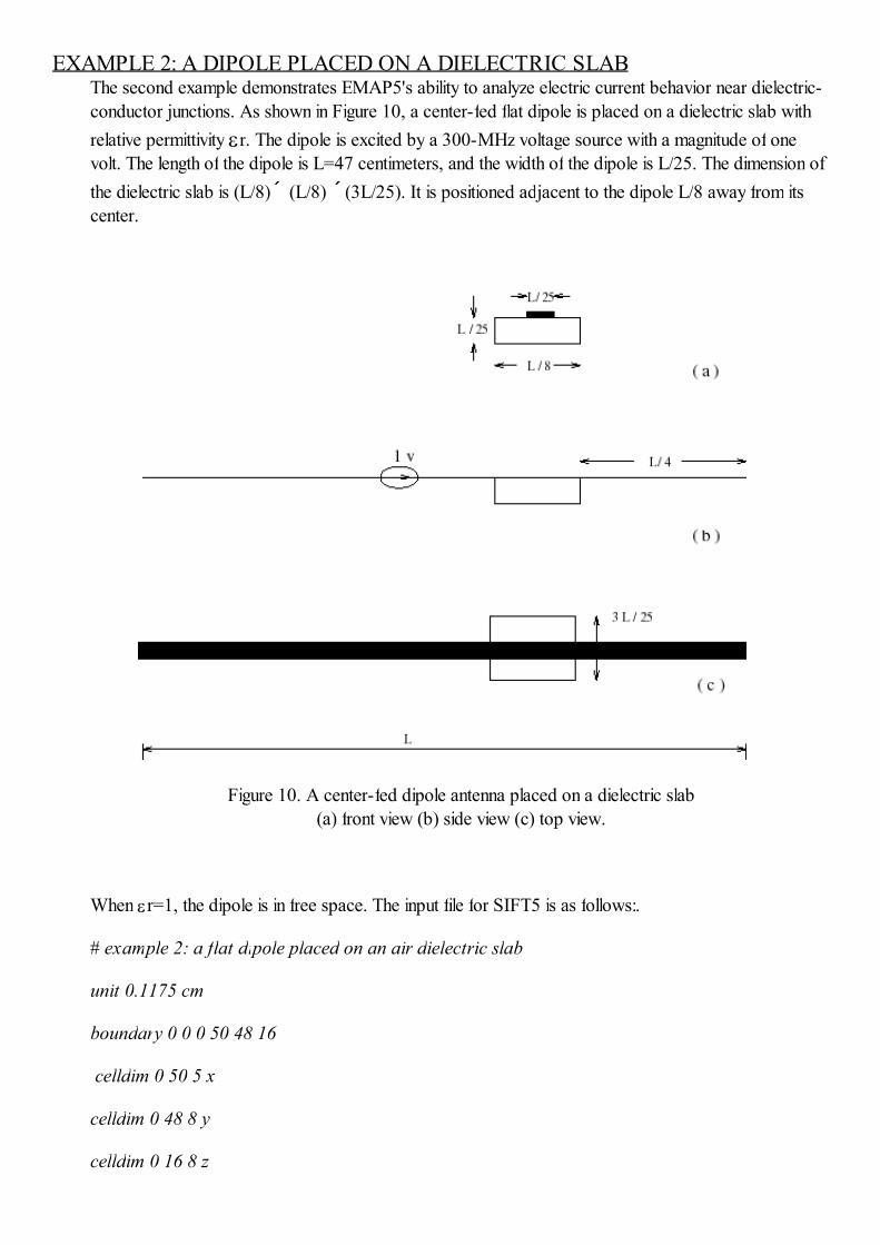
conductor junctions. As shown in Figure 10, a center-fed flat dipole is placed on a dielectric slab with
relative permittivity εr. The dipole is excited by a 300-MHz voltage source with a magnitude of one
volt. The length of the dipole is L=47 centimeters, and the width of the dipole is L/25. The dimension of
the dielectric slab is (L/8)´ (L/8) ´(3L/25). It is positioned adjacent to the dipole L/8 away from its
center.
Figure 10. A center-fed dipole antenna placed on a dielectric slab
(a) front view (b) side view (c) top view.
When εr=1, the dipole is in free space. The input file for SIFT5 is as follows:.
# example 2: a flat dipole placed on an air dielectric slab
unit 0.1175 cm
boundary 0 0 0 50 48 16
celldim 0 50 5 x
celldim 0 48 8 y
celldim 0 16 8 z
dielectric 0 0 0 50 48 16 1.0 0.0
conductor -250 16 16 150 32 16 5 8 8
vsource -50 16 16 -50 32 16 300 x 1.0
output -250 16 16 0 32 16 y example2.out
output 50 16 16 150 32 16 y example2.out
The structure is divided into 600 tetrahedra and 648 triangles. The total number of unknowns is 966
after the MoM equation is coupled to the FEM equation. Eight edges are used to model the behavior of
the currents in the junction ar eas.
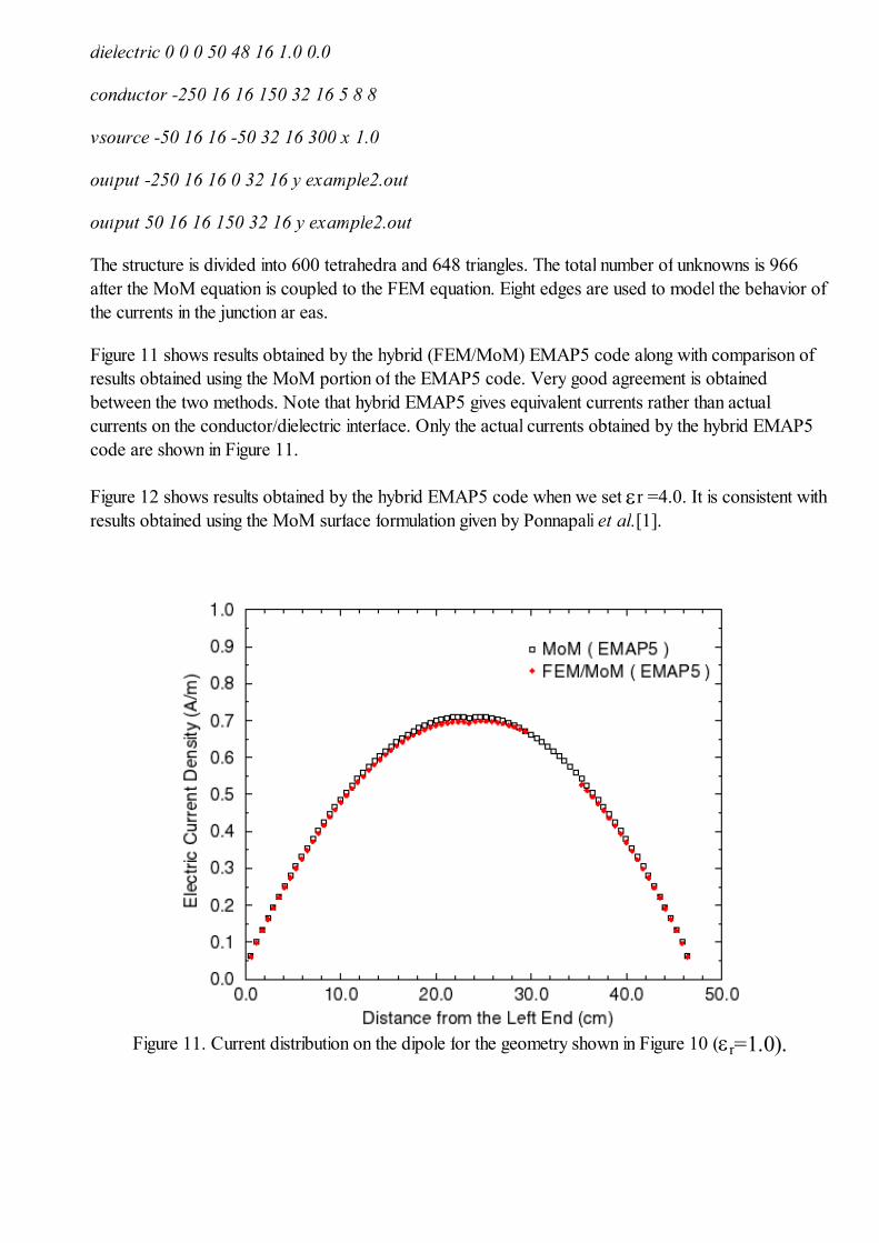
Figure 11 shows results obtained by the hybrid (FEM/MoM) EMAP5 code along with comparison of
results obtained using the MoM portion of the EMAP5 code. Very good agreement is obtained
between the two methods. Note that hybrid EMAP5 gives equivalent currents rather than actual
currents on the conductor/dielectric interface. Only the actual currents obtained by the hybrid EMAP5
code are shown in Figure 11.
Figure 12 shows results obtained by the hybrid EMAP5 code when we set εr =4.0. It is consistent with
results obtained using the MoM surface formulation given by Ponnapali et al.[1].
Figure 11. Current distribution on the dipole for the geometry shown in Figure 10 (εr=1.0).
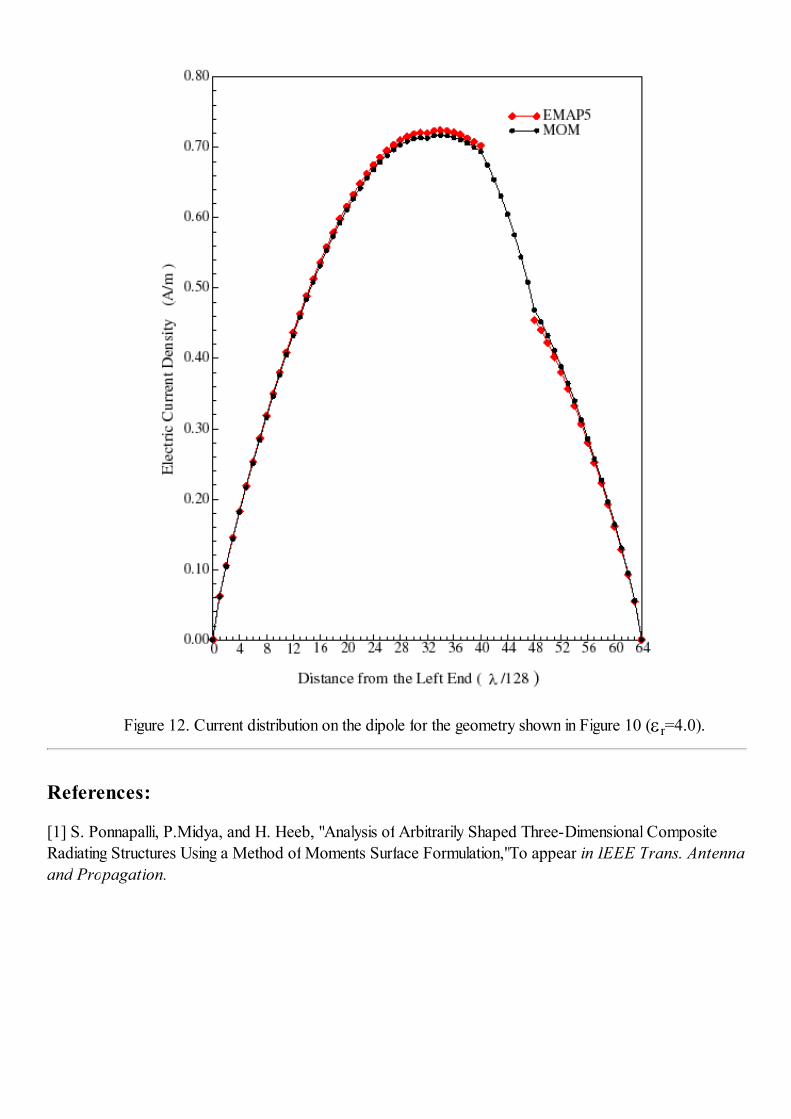
Figure 12. Current distribution on the dipole for the geometry shown in Figure 10 (εr=4.0).
References:
[1] S. Ponnapalli, P.Midya, and H. Heeb, "Analysis of Arbitrarily Shaped Three-Dimensional Composite
Radiating Structures Using a Method of Moments Surface Formulation,"To appear in IEEE Trans. Antenna
and Propagation.