ECON4510 Finance TheoryLecture 9

Kjetil StoreslettenDepartment of EconomicsUniversity of OsloApril 20, 2017

1

Empirical Tests of theCapital Asset Pricing Model

Traditional Tests of the CAPM Black, Jensen, and Scholes Study Fama and MacBeth Study Roll’s Critique of Tests of the CAPM Additional Evidence

Traditional Tests of the CAPM

The CAPM predicts that all investors hold portfolios that are efficient in expected return, standard deviation space. Therefore, the Market Portfolio is efficient. To test the CAPM, we must test the prediction that the Market Portfolio is positioned on the efficient set.

Initial testing of the CAPM did not test directly the prediction, “The Market Portfolio is efficient.” Instead, researchers followed the theme, “If a linear positive relationship exists between portfolio return and beta, the Market Portfolio must be efficient.”

Traditional Tests of the CAPM (Continued)

Two classical traditional studies:

– Black, F., Jensen, M. C., & Scholes, M. “The Capital Asset Pricing Model: Some Empirical Tests,” in Ed. Jensen, M. C. Studies in Theory of Capital Markets.New York: Praeger, 1972.

– Fama, E. F., & MacBeth, J., “Tests of Multiperiod Two Parameter Model,” Journal of Political Economy (May 1974).

Black, Jensen, and Scholes Study

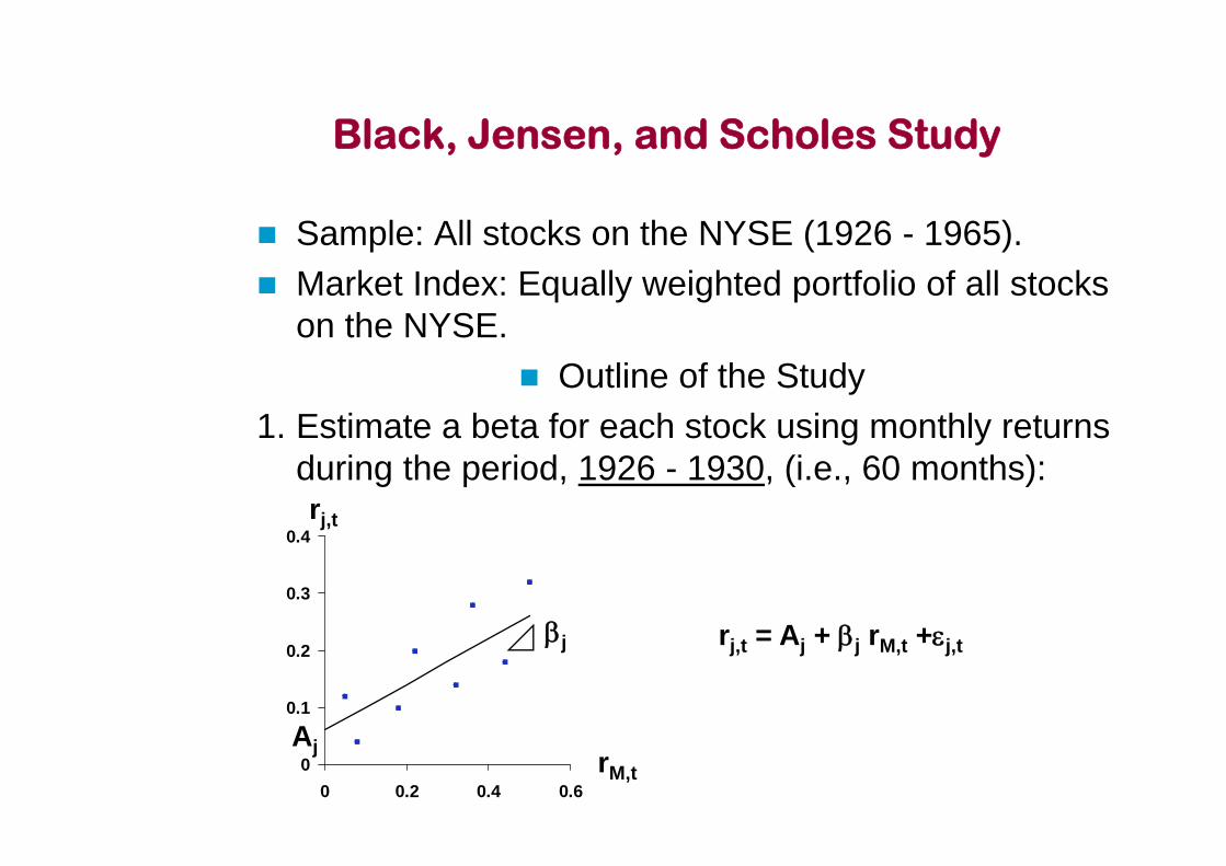
Sample: All stocks on the NYSE (1926 - 1965). Market Index: Equally weighted portfolio of all stocks

on the NYSE. Outline of the Study

1. Estimate a beta for each stock using monthly returns during the period, 1926 - 1930, (i.e., 60 months):

0

0.1

0.2

0.3

0.4

0 0.2 0.4 0.6

rj,t

rM,t

rj,t = Aj + j rM,t +j,tj

Aj

2. Rank order all of the stock betas, and form 10 portfolios:– Top 10% with the highest betas comprise

portfolio #1, next 10% portfolio #2, . . . and so forth until portfolio #10 contains the bottom 10% with the smallest betas.

3. Compute each of the portfolio’s returns for eachof the 12 months in 1931:

n

r

r

n

1jtj,

tp,

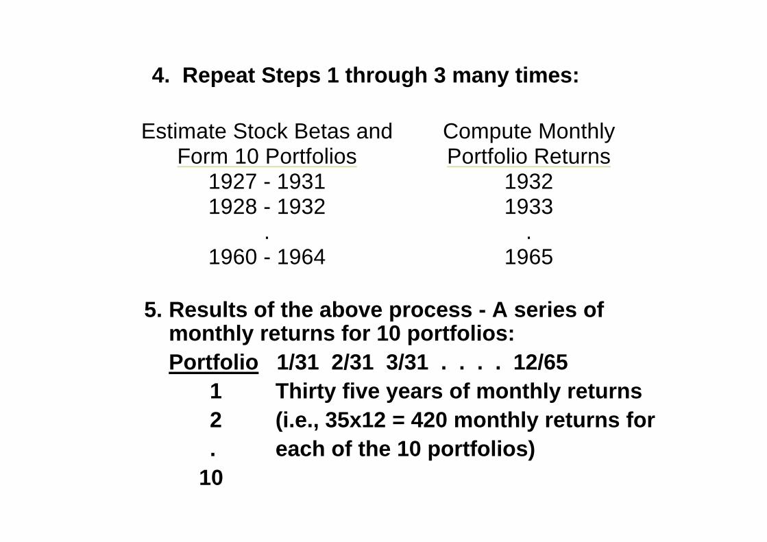
4. Repeat Steps 1 through 3 many times:

5. Results of the above process - A series of monthly returns for 10 portfolios:Portfolio 1/31 2/31 3/31 . . . . 12/65

1 Thirty five years of monthly returns2 (i.e., 35x12 = 420 monthly returns for. each of the 10 portfolios)

10

Estimate Stock Betas andForm 10 Portfolios

1927 - 19311928 - 1932

.1960 - 1964

Compute MonthlyPortfolio Returns

19321933

.1965

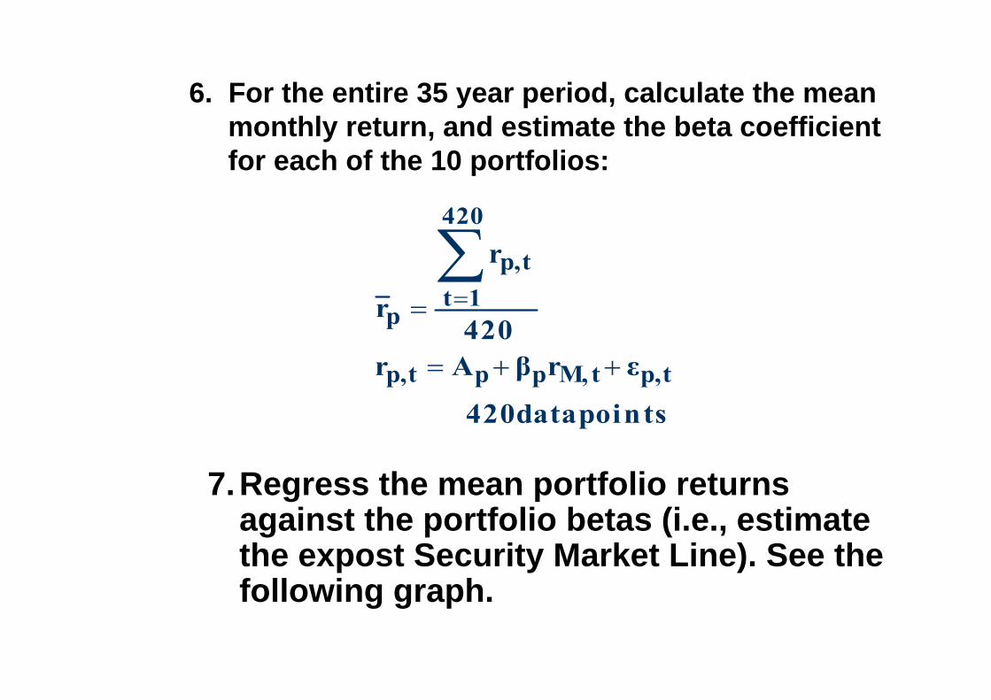
6. For the entire 35 year period, calculate the meanmonthly return, and estimate the beta coefficient for each of the 10 portfolios:

7.Regress the mean portfolio returns against the portfolio betas (i.e., estimate the expost Security Market Line). See the following graph.

points data 420

εrβAr420

r

r

tp,tM,pptp,

420

1ttp,

p

BJS Ex Post Security Market Line (SML)

9

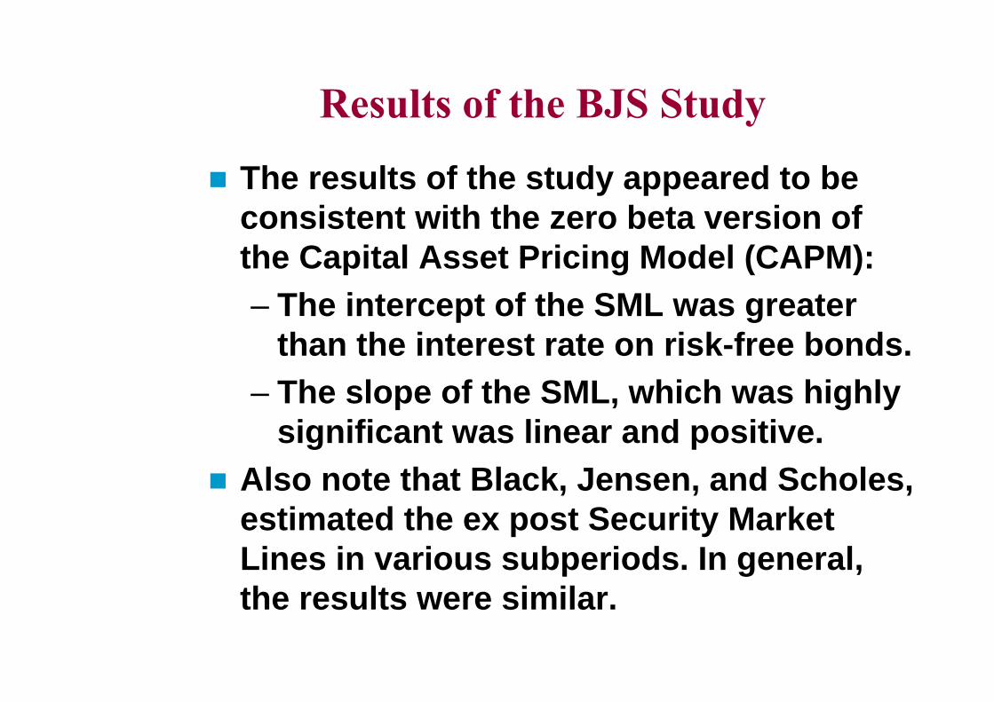
Results of the BJS Study

The results of the study appeared to be consistent with the zero beta version of the Capital Asset Pricing Model (CAPM):– The intercept of the SML was greater

than the interest rate on risk-free bonds.– The slope of the SML, which was highly

significant was linear and positive. Also note that Black, Jensen, and Scholes,

estimated the ex post Security Market Lines in various subperiods. In general, the results were similar.

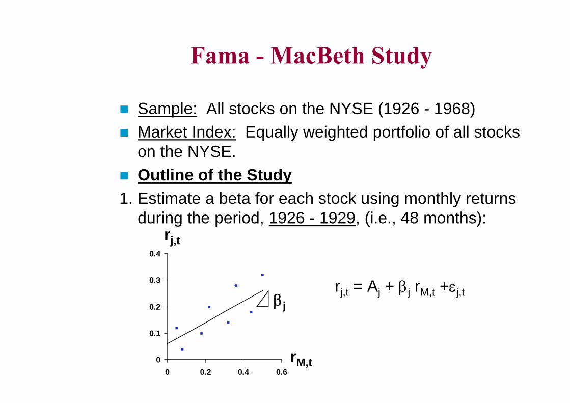
Fama - MacBeth Study

Sample: All stocks on the NYSE (1926 - 1968) Market Index: Equally weighted portfolio of all stocks

on the NYSE. Outline of the Study1. Estimate a beta for each stock using monthly returns

during the period, 1926 - 1929, (i.e., 48 months):

rj,t = Aj + j rM,t +j,t

0

0.1

0.2

0.3

0.4

0 0.2 0.4 0.6

rj,t

rM,t

j

2. Rank order all of the stock betas, and form 20portfolios. The top 5% with the highest betas are inportfolio #1, . . . etc. . . the bottom 5% with thesmallest betas are in portfolio #20.

3. Estimate the beta of each of the portfolios by regressing portfolio monthly returns against the market index during the period, 1930 - 1934, (i.e., 60 months):

rp,t = Ap + p rM,t +p,t

rp,t

rM,t

p

Ap

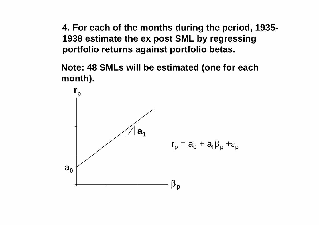
4. For each of the months during the period, 1935-1938 estimate the ex post SML by regressing portfolio returns against portfolio betas.

Note: 48 SMLs will be estimated (one for each month).

rp = a0 + ap +p

rp

p

a1

a0

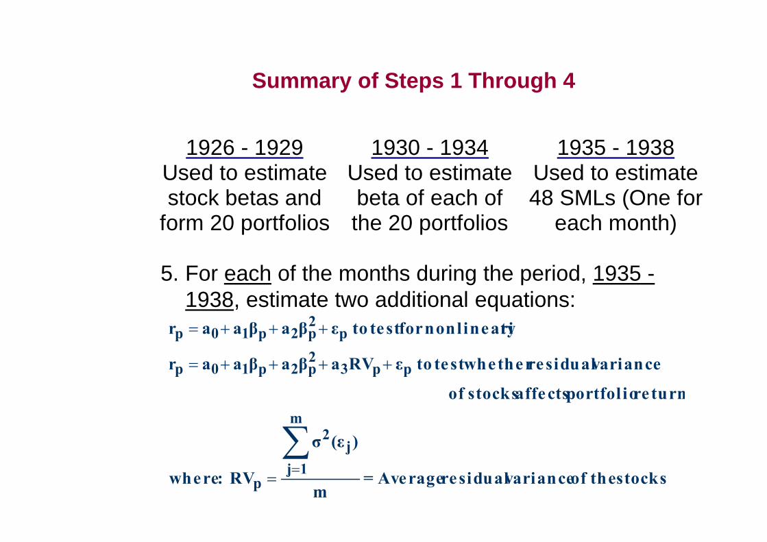
Summary of Steps 1 Through 4

5. For each of the months during the period, 1935 -1938, estimate two additional equations:

1926 - 1929 Used to estimatestock betas and

form 20 portfolios

1930 - 1934 Used to estimate beta of each of the 20 portfolios

1935 - 1938 Used to estimate 48 SMLs (One for

each month)

stocks the of variance residual Average= m

)(εσ

RV :where

re turn portfol io affects stocks of

variance residualwhether te st to εRVaβaβaar

tynonlinearifor te st to εβaβaar

m

1jj

2

p

pp32p2p10p

p2p2p10p

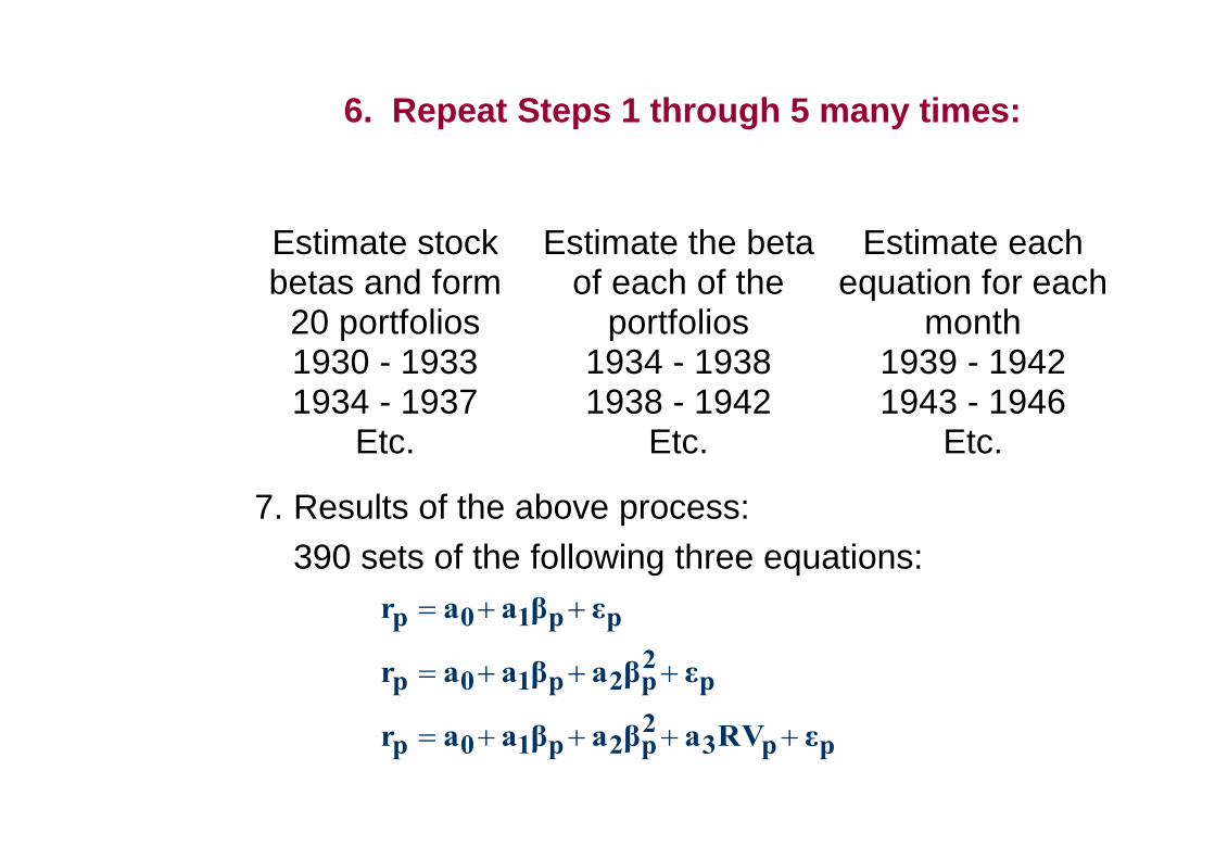
6. Repeat Steps 1 through 5 many times:

7. Results of the above process:390 sets of the following three equations:

Estimate stockbetas and form

20 portfolios1930 - 19331934 - 1937

Etc.

Estimate the betaof each of the

portfolios1934 - 19381938 - 1942

Etc.

Estimate eachequation for each

month1939 - 19421943 - 1946

Etc.

pp32p2p10p

p2p2p10p

pp10p

εRVaβaβaar

εβaβaar

εβaar

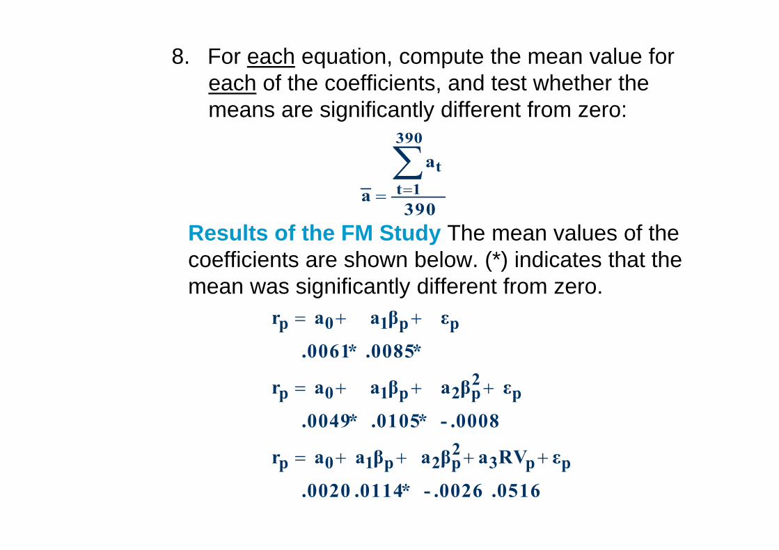
8. For each equation, compute the mean value for each of the coefficients, and test whether themeans are significantly different from zero:

Results of the FM Study The mean values of the coefficients are shown below. (*) indicates that the mean was significantly different from zero.

390

a

a

390

1tt

.0516 .0026- *.0114 .0020

ε RVa βa βa a r

.0008- *.0105 *.0049

ε βa βa a r

*.0085 *.0061

ε βa a r

pp32p2p10p

p2p2p10p

pp10p

The FM results appeared to be consistent with the zero beta version of the CAPM:

– a0 was significantly greater than the mean of the risk-free interest rate.

– a1 was significantly different from zero. The slope of the SML was positive.

– a2 and a3 were not significantly different from zero (i.e., there was no evidence of nonlinearity or of residual variance affecting returns).

Difference between BJS and FM Studies– In BJS, betas and average returns were

computed in the same periods.– In FM, betas in one period were used to

predict returns in a later period.

Roll’s Critique of Tests of the CAPM

Tests like those of BJS and FM are tautological (not necessary). Results like those reported could be obtained irrespective of how securities were priced relative to risk. (e.g., pulling numbers out of a hat would produce the same results). Therefore, the CAPM was not really tested. Furthermore, since we cannot operationally define the market portfolio, the CAPM can never be tested.

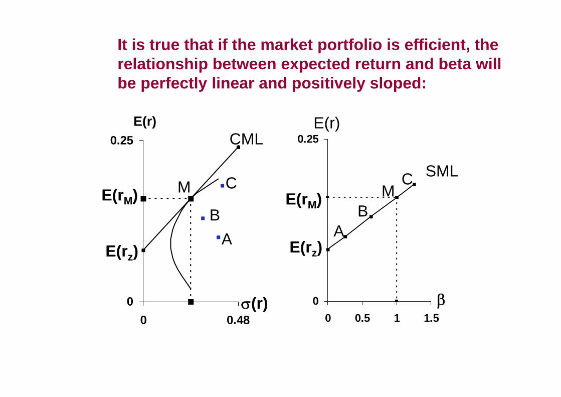
It is true that if the market portfolio is efficient, the relationship between expected return and beta will be perfectly linear and positively sloped:

0

0.25

0 0.480

0.25

0 0.5 1 1.5

E(r)

E(rM)

E(rz)

E(rM)

E(rz)

E(r)

(r)

SML

CML

M C

BA

CM

BA

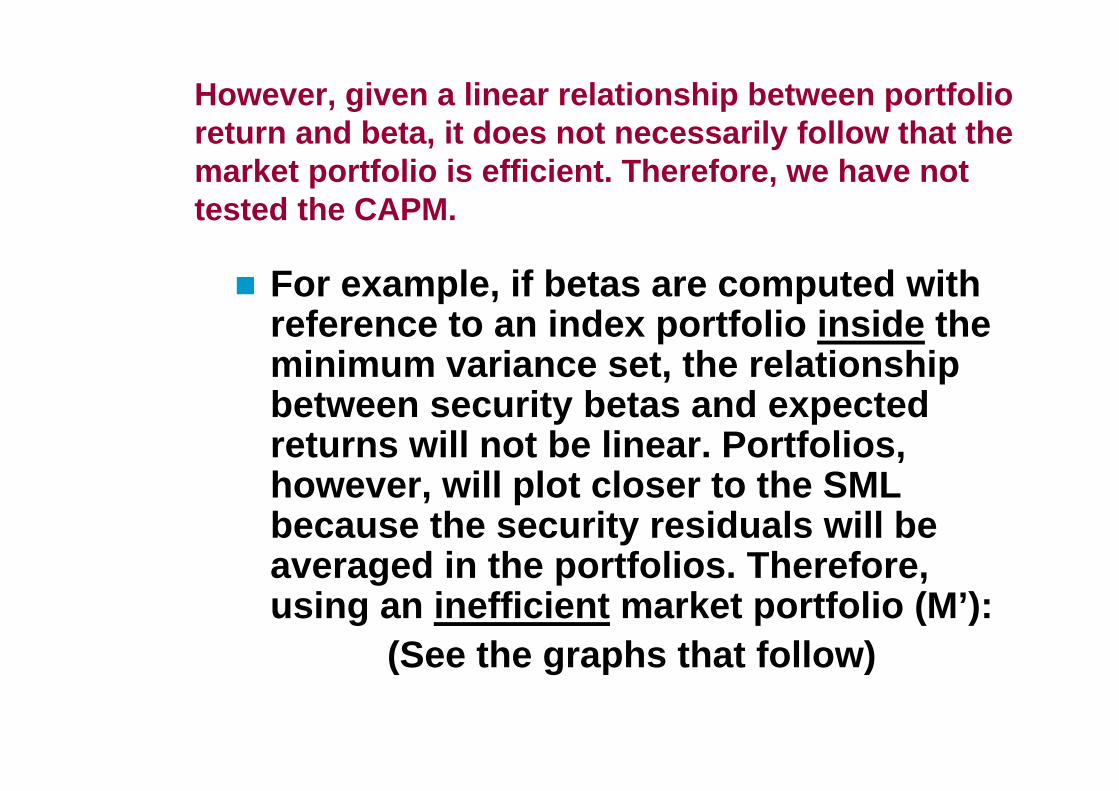
However, given a linear relationship between portfolio return and beta, it does not necessarily follow that the market portfolio is efficient. Therefore, we have not tested the CAPM.

For example, if betas are computed with reference to an index portfolio inside the minimum variance set, the relationship between security betas and expected returns will not be linear. Portfolios, however, will plot closer to the SML because the security residuals will be averaged in the portfolios. Therefore, using an inefficient market portfolio (M’):

(See the graphs that follow)

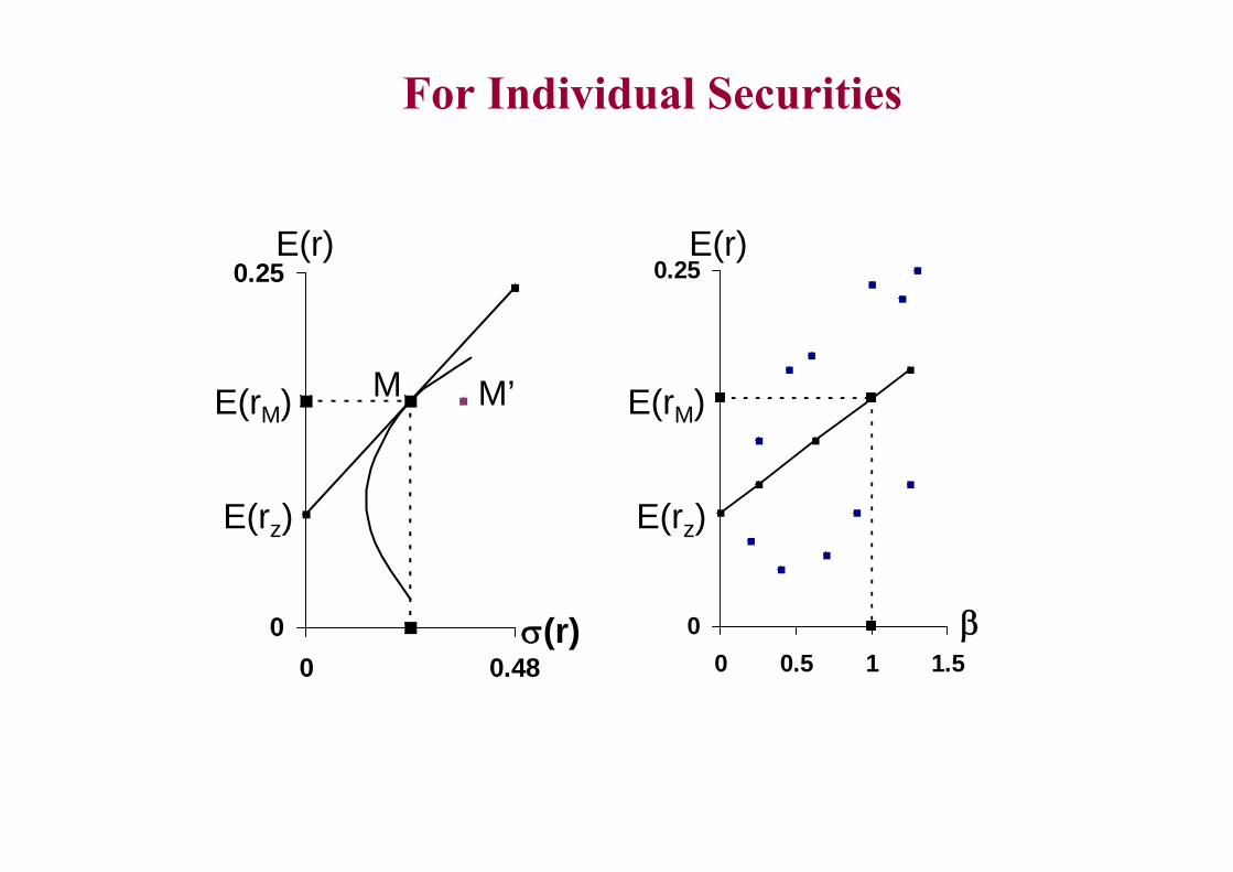
For Individual Securities

0

0.25

0 0.480

0.25

0 0.5 1 1.5

E(r)

E(rM)

E(rz)

M

(r)

E(rM)

E(rz)

E(r)

M’

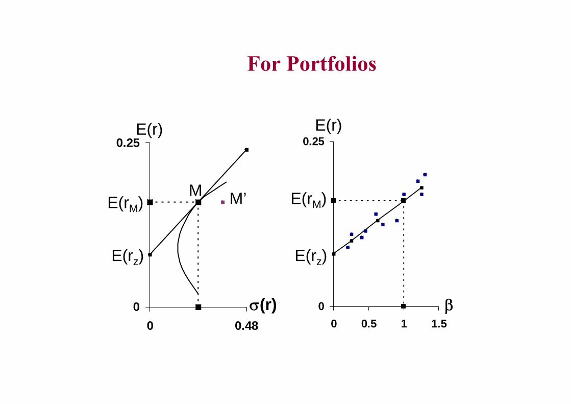
For Portfolios

0

0.25

0 0.480

0.25

0 0.5 1 1.5

E(r)

E(rM)

E(rz)

M

(r)

E(rM)

E(rz)

E(r)

M’

Some Recent Controversial Evidence

Fama/French Study– Small firms tend to outperform large firms.– Stocks with low ratios of price to book

value tend to outperform stocks with high ratios of price to book value.

– The relationship between return and beta was essentially flat to negative.

On the Other Hand . . Some Argued . . .

Fama and French study suffers from “survival bias.”– Many stocks with low ratios of price to

book value are in financial stress and wind up failing. These stocks were excluded from the Fama and French data. This produced upward bias in the performance of low price to book value stocks as a class.

Still Others Argued . . .

The impact of survival bias does not fully explain the relationship found between performance and the price to book value ratio.

Irrespective of the price to book value ratio, survival bias cannot be used to explain the flat to negative relationship between return and beta.

Comment on Testing the CAPM

The evidence discussed above does not prove that the CAPM is invalid since only stocks were included in the analyses. The “Market Portfolio” contains all of the capital assets in the universe. We will never be able to observe the returns on the “true” Market Portfolio. Therefore, the CAPM is simply not a testable theory.

Some Additional Evidence

Estimated betas are very sensitive to the market index being used.

In risk-return space, indices can be close to each other, and close to the efficient set, and still produce different relationships (positive and negative) between return and beta.

One study suggested using a dual beta approach to adjust for risk differences in bull and bear markets.