Detecting the direction of a signal on high-dimensional ...

Noname manuscript No.(will be inserted by the editor)

Detecting the direction of a signal onhigh-dimensional spheres

Non-null and Le Cam optimality results

Davy Paindaveine · Thomas Verdebout

Received: date / Accepted: date

Abstract We consider one of the most important problems in directionalstatistics, namely the problem of testing the null hypothesis that the spikedirection θθθ of a Fisher–von Mises–Langevin distribution on the p-dimensionalunit hypersphere is equal to a given direction θθθ0. After a reduction throughinvariance arguments, we derive local asymptotic normality (LAN) results ina general high-dimensional framework where the dimension pn goes to infinityat an arbitrary rate with the sample size n, and where the concentration κnbehaves in a completely free way with n, which offers a spectrum of problemsranging from arbitrarily easy to arbitrarily challenging ones. We identify vari-ous asymptotic regimes, depending on the convergence/divergence propertiesof (κn), that yield different contiguity rates and different limiting experiments.In each regime, we derive Le Cam optimal tests under specified κn and we com-pute, from the Le Cam third lemma, asymptotic powers of the classical Watsontest under contiguous alternatives. We further establish LAN results with re-spect to both spike direction and concentration, which allows us to discussoptimality also under unspecified κn. To investigate the non-null behavior ofthe Watson test outside the parametric framework above, we derive its local

Research is supported by the Program of Concerted Research Actions (ARC) of the Univer-site libre de Bruxelles, by a research fellowship from the Francqui Foundation, and by theCredit de Recherche J.0134.18 of the FNRS (Fonds National pour la Recherche Scientifique),Communaute Francaise de Belgique.

Davy PaindaveineUniversite libre de Bruxelles, ECARES and Departement de Mathematique, Avenue F.D.Roosevelt, 50, ECARES, CP114/04, B-1050, Brussels, BelgiumTel.: +3226503845E-mail: [email protected]

Thomas VerdeboutUniversite libre de Bruxelles, ECARES F.D. Departement de Mathematique, Avenue F.D.Roosevelt, 50, ECARES, CP114/04, B-1050, Brussels, BelgiumTel.: +3226505892E-mail: [email protected]

2 Davy Paindaveine, Thomas Verdebout

asymptotic powers through martingale CLTs in the broader, semiparametric,model of rotationally symmetric distributions. A Monte Carlo study showsthat the finite-sample behaviors of the various tests remarkably agree withour asymptotic results.

Keywords High-dimensional statistics · invariance · Le Cam’s asymptotictheory of statistical experiments · local asymptotic normality · rotationallysymmetric distributions

Mathematics Subject Classification (2010) 62H11 · 62F05 · 62G10

1 Introduction

In directional statistics, the sample space is the unit sphere Sp−1 = {x ∈ Rp :‖x‖2 = x′x = 1} in Rp. By far the most classical distributions on Sp−1 are theFisher–von Mises–Langevin (FvML) ones; see, e.g., [27] or [28]. We say thatthe random vector X with values in Sp−1 has an FvMLp(θθθ, κ) distribution,with θθθ ∈ Sp−1 and κ ∈ (0,∞), if it admits the density (throughout, densitieson the unit sphere are with respect to the surface area measure)

x 7→ cp,κωp−1

exp(κx′θθθ), (1.1)

where, denoting as Γ (·) the Euler Gamma function and as Iν(·) the order-νmodified Bessel function of the first kind, ωp := (2πp/2)/Γ

(p2

)is the surface

area of Sp−1 and

cp,κ := 1/∫ 1

−1(1− t2)(p−3)/2 exp(κt) dt =

(κ/2)(p/2)−1√π Γ(p−12

)I p

2−1(κ)·

Clearly, θθθ is a location parameter (θθθ is the modal location on the sphere),that identifies the spike direction of the hyperspherical signal. In contrast, κis a scale or concentration parameter: the larger κ, the more concentratedthe distribution is about the modal location θθθ. As κ converges to zero, cp,κconverges to cp := Γ

(p2

)/(√π Γ(p−12

)) and the density in (1.1) converges

to the density x 7→ 1/ωp of the uniform distribution over Sp−1. The otherextreme case, obtained for arbitrarily large values of κ, provides distributionsthat converge to a point mass in θθθ. Of course, it is expected that the larger κ,the easier it is to conduct inference on θθθ — that is, the more powerful the testson θθθ and the smaller the corresponding confidence zones.

In this paper, we consider inference on θθθ and focus on the generic testingproblem for which the null hypothesis H0 : θθθ = θθθ0, for a fixed θθθ0 ∈ Sp−1, is tobe tested against H1 : θθθ 6= θθθ0 on the basis of a random sample Xn1, . . . ,Xnn

from the FvMLp(θθθ, κ) distribution — the triangular array notation antici-pates non-standard setups where p (hence, also θθθ) and/or κ will depend on n.Inference problems on θθθ in the low-dimensional case have been consideredamong others in [8], [9], [17], [19], [22], [26], [31] and [37]. The related spherical

Detecting the direction of a signal on high-dimensional spheres 3

regression problem has been tackled in [14] and [33], while testing for locationon axial frames has been considered in [2].

Letting Xn := 1n

∑ni=1 Xni, the most classical test for the testing problem

above is the Watson [37] test rejecting the null at asymptotic level α whenever

Wn :=n(p− 1)X′n(Ip − θθθ0θθθ′0)Xn

1− 1n

∑ni=1(X′niθθθ0)2

> χ2p−1,1−α, (1.2)

where I` stands for the `-dimensional identity matrix and χ2`,1−α denotes the

α-upper quantile of the chi-square distribution with ` degrees of freedom. Inthe classical setup where p and κ are fixed, the asymptotic properties of theWatson test are well-known, both under the null and under local alternatives;see, e.g., [28] or [37]. Optimality properties in the Le Cam sense have beenstudied in [30]. In the non-standard setup where κ = κn converges to zero,[31] investigated the asymptotic null and non-null behaviors of the Watsontest. Interestingly, irrespective of the rate at which κn converges to zero (thatis, irrespective of how fast the inference problem becomes more challengingas a function of n), the Watson test keeps meeting the asymptotic nominallevel constraint and maintains strong optimality properties; see [31] for details.In the other non-standard, high-concentration, setup where κn diverges toinfinity, [32] showed the Watson test also enjoys strong optimality properties.

For a fixed dimension p, this essentially settles the investigation of theproperties of the Watson test and the study of the corresponding hypothe-sis testing problem. Nowadays, however, increasingly many applications leadto considering high-dimensional directional data: tests of uniformity on high-dimensional spheres have been studied in [7], [10], [11] and [12], while high-dimensional FvML distributions (or mixtures of high-dimensional FvML dis-tributions) have been considered in magnetic resonance, gene-expression, andtext mining; see, among others, [3], [4] and [15]. This motivates consideringthe high-dimensional spherical location problem, based on a random sam-ple Xn1, . . . ,Xnn from the FvMLpn(θθθn, κn) distribution, with (pn) divergingto infinity (the dimension of θθθn then depends on n, which justifies the nota-tion). In this context, it was proved in [25] that the Watson test is robust tohigh-dimensionality in the sense that, as pn goes to infinity with n, this teststill has asymptotic size α under H(n)

0 : θθθn = θθθn0. This does not require anycondition on the concentration sequence (κn) nor on the rate at which pn goesto infinity, hence covers arbitrarily easy problems (κn large) and arbitrarilychallenging ones (κn small), as well as moderately high dimensions and ultra-high dimensions. On its own, however, this null robustness result is obviouslyfar from sufficient to motivate using the Watson test in high dimensions, as itmight very well be that robustness under the null is obtained at the expenseof power (in the extreme case, the Watson test, in high dimensions, might ac-tually asymptotically behave like the trivial α-level test that randomly rejectsthe null with probability α).

These considerations raise many interesting questions, among which: arethere alternatives under which the Watson test is consistent in high dimen-sions? What are the less severe alternatives (if any) under which the Watson


test exhibits non-trivial asymptotic powers? Is the Watson test rate-optimal or,on the contrary, are there tests that show asymptotic powers under less severealternatives than those detected by the Watson test? Does the Watson testenjoy optimality properties in high dimensions? As we will show, answeringthese questions will require considering several regimes fixing how the concen-tration κn behaves as a function of the dimension pn and sample size n. Ourresults, that will crucially depend on the regime considered, are extensive inthe sense that they answer the questions above in all possible regimes.

Our results will rely on two different approaches. (a) The first approach isbased on Le Cam’s asymptotic theory of statistical experiments. While thistheory is very general, it does not directly apply in the present context sincethe high-dimensional spherical location problem involves a parametric space,namely {(θθθn, κ) : θθθn ∈ Spn−1, κ ∈ (0,∞)}, that depends on n (through pn).We solve this by exploiting the invariance properties of the testing problemconsidered. In the image of the model by the corresponding maximal invari-ant, indeed, the parametric space does not depend on n anymore, which opensthe door to studying the problem through the Le Cam approach. We derivestochastic second-order expansions of the resulting log-likelihood ratios, whichis the main technical ingredient to establish the local asymptotic normality(LAN) of the invariant model. The LAN property takes different forms andinvolves different contiguity rates depending on the regime that is considered.In each regime, we determine the Le Cam optimal test for the problem con-sidered and apply the Le Cam third lemma to obtain the asymptotic powersof this test and of the Watson test. This allows us to determine the regime(s)in which the Watson test is Le Cam optimal, or only rate-optimal, or not evenrate-optimal. While this is first done under specified concentration κn, we fur-ther provide LAN results with respect to both location and concentration tobe able to discuss optimality under unspecified κn. (b) While our investiga-tion in (a) will fully characterize the asymptotic optimality properties of theWatson test in the FvML case, it will not provide any insight on the non-null behavior of this test outside this stringent parametric framework. Thismotivates complementing our investigation by a second approach, based onmartingale CLTs. We will consider a broad, semiparametric, model, namelythe class of rotationally symmetric distributions, and will identify the alter-natives (if any) under which the Watson test will show non-trivial asymptoticpowers in high dimensions. Again, this requires considering various regimesaccording to the concentration pattern.

The outline of the paper is as follows. In Section 2, we consider the high-dimensional version of the FvML spherical location problem. In Section 2.1,we describe the invariance approach that allows us to later rely on Le Cam’sasymptotic theory of statistical experiments. In Section 2.2, we provide astochastic second-order expansion of the resulting invariant log-likelihood ra-tios and prove, in various regimes that we identify, that these invariant modelsare locally asymptotically normal. This allows us to derive the correspondingLe Cam optimal tests for the specified concentration problem and to study thenon-null asymptotic behavior of the Watson test in the light of these results.


In Section 2.3, we tackle the unspecified concentration problem through thederivation of LAN results that are with respect to both location and concen-tration. In Section 3, we conduct a systematic investigation of the non-nullasymptotic properties of the Watson test in the broader context of rotation-ally symmetric distributions. This in particular confirms the FvML resultsobtained in Section 2. In Section 4, we conduct a Monte Carlo study to in-vestigate how well the finite-sample behaviors of the various tests reflect ourtheoretical asymptotic results. In Section 5, we summarize the results obtainedin the paper and shortly discuss research perspectives. Finally, an appendixcontains all proofs.

2 Invariance and Le Cam optimality

As already mentioned in the introduction, the high-dimensional spherical lo-cation problem requires considering triangular arrays of observations of theform Xni, i = 1, . . . , n, n = 1, 2, . . . For any sequence (θθθn) such that θθθn be-longs to Spn−1 for any n and any sequence (κn) in (0,∞), we denote as P

(n)θθθn,κn

the hypothesis under which Xni, i = 1, . . . , n, form a random sample from theFvMLpn(θθθn, κn) distribution. The resulting sequence of statistical models isthen associated with

P(n) ={

P(n)θθθn,κ

: (θθθn, κ) ∈ ΘΘΘn := Spn−1 × (0,∞)}

(2.3)

(the index in the parameter θθθn in principle is superfluous but is used hereto stress the dependence of this parameter on pn, hence on n). The spheri-

cal location problem consists in testing the null hypothesis H(n)0 : θθθn = θθθn0

against the alternative H(n)0 : θθθn 6= θθθn0, where (θθθ0n) is a fixed sequence such

that θθθ0n belongs to Spn−1 for any n. Clearly, θθθn is the parameter of interest,whereas κn plays the role of a nuisance. Our main objective in this section isto derive Le Cam optimality results for this problem, referring to sequences

of local alternatives of the form P(n)θθθn,κn

, with θθθn = θθθn0 + νnτττn, where the se-

quence (νn) and the bounded sequence (τττn), respectively in (0,∞) and Rpn ,are such that θθθn ∈ Spn−1 for any n, which imposes that

θθθ′n0τττn = −1

2νn‖τττn‖2 (2.4)

for any n; throughout, “the sequence (τττn) in Rpn is bounded” means that τττn ∈Rpn for any n and that ‖τττn‖ = O(1) as n→∞. The obvious lack of identifia-bility of νn and τττn will be no problem in the sequel (only the locally perturbedparameter values θθθn = θθθ0+νnτττn are of interest, hence not the individual quan-tities νn and τττn themselves) and this form of local alternatives is actually thestandard one in the Le Cam theory; see, e.g., Chapter 6 in [23] or Defini-tion 7.14 in [36]. Whenever local asymptotic powers will be considered below,we will assume that ‖τττn‖ is O(1) without being o(1), so that νn will charac-terize (the rate of) the severity of the local alternatives θθθn = θθθ0 + νnτττn (theslower νn goes to zero, the more severe the corresponding local alternatives).


Since the sequence of “statistical experiments” associated with (2.3) in-volves parametric spaces ΘΘΘn that depend on n, applying Le Cam’s theory willrequire the following reduction of the problem through invariance arguments.

2.1 Reduction through invariance

Denoting as SOp(θθθ) the collection of p×p orthogonal matrices satisfying Oθθθ =

θθθ, the null hypothesis H(n)0 is invariant under the group Gn, ◦ collecting the

transformations

(Xn1, . . . ,Xnn) 7→ gnO(Xn1, . . . ,Xnn) = (OXn1, . . . ,OXnn),

with O ∈ SOpn(θθθn0). The transformation gnO induces a transformation of theparametric space ΘΘΘn defined through (θθθn, κ) 7→ (Oθθθn, κ). The orbits of theresulting induced group are Cu,κ(θθθn0) := {θθθn ∈ Spn−1 : θθθ′nθθθn0 = u} × {κ},with u ∈ [−1, 1] and κ ∈ (0,∞). In such a context, the invariance principle(see, e.g., [24], Chapter 6) leads to restricting to tests φn that are invariant withrespect to the group Gn,◦. Denoting as Tn = Tn(Xn1, . . . ,Xnn) a maximalinvariant statistic for Gn,◦, the class of invariant tests coincides with the classof Tn-measurable tests. Invariant tests thus are to be defined in the image

P(n)Tn ={

P(n)Tnu,κ : (u, κ) ∈ ΨΨΨ := [−1, 1]× (0,∞)

}(2.5)

of the model P(n) by Tn, where P(n)Tnu,κ denotes the common distribution

of Tn under any P(n)θθθn,κ

with (θθθn, κ) ∈ Cu,κ(θθθn0). Unlike the original sequence

of statistical experiments in (2.3), the invariant one in (2.5) involves a fixedparametric space ΨΨΨ , which makes it in principle possible to rely on Le Cam’sasymptotic theory.

Now, the original local log-likelihood ratios log(dP(n)θθθn,κn

/dP(n)θθθn0,κn

) associ-ated with the generic local alternatives θθθn = θθθn0 + νnτττn above correspond, inview of (2.4), to the invariant local log-likelihood ratios

Λ(n)invθθθn/θθθn0;κn

:= logdP

(n)Tn1−ν2

n‖τττn‖2/2,κn

dP(n)Tn1,κn

· (2.6)

Deriving local asymptotic normality (LAN) results requires investigating theasymptotic behavior of such invariant log-likelihood ratios, which in turn re-quires evaluating the corresponding likelihoods. While obtaining a closed-formexpression for Tn and its distribution is a very challenging task, these likeli-hoods can be obtained from Lemma 2.5.1 in [16], which, denoting as mn the


surface area measure on Spn−1 × . . .× Spn−1 (n times), yields

dP(n)Tn1−ν2

n‖τττn‖2/2,κndmn

=

∫SOpn (θθθn0)

dP(n)θθθn,κn

dmn(OXn1, . . . ,OXnn) dO

=

∫SOpn (θθθn0)

n∏i=1

(cpn,κnωpn−1

exp(κn(OXni)

′θθθn))

dO

=cnpn,κnωnpn−1

∫SOpn (θθθn0)

exp(nκnXnO′θθθn

)dO, (2.7)

where integration is with respect to the Haar measure on SOpn(θθθn0). Note

that (2.7) shows that the invariant null probability measure P(n)Tn1,κn

coincideswith the original null probability measure P

(n)θθθn0,κn

. In other words, it is onlyfor non-null probability measures that the invariance reduction above is non-trivial.

2.2 Optimal testing under specified κn

The main ingredient needed to obtain LAN results is Theorem 1 below, thatprovides a stochastic second-order expansion of the invariant log-likelihoodratios in (2.6). To state this theorem, we need to introduce the following no-tation. We will refer to the decomposition Xni = Uniθθθn0 + VniSn, with

Uni = X′niθθθn0, Vni = (1− U2ni)

1/2 and Sni =(Ipn − θθθn0θθθ

′n0)Xni

‖(Ipn − θθθn0θθθ′n0)Xni‖

,

as the tangent-normal decomposition of Xni with respect to θθθn0. Under the

hypothesis P(n)θθθn0,κn

, Uni has probability density function

u 7→ cpn,κn(1− u2)(pn−3)/2 exp(κnu) I[u ∈ [−1, 1]], (2.8)

where I[A] denotes the indicator function of A, Sni is uniformly distributedover the “equator” {x ∈ Spn−1 : x′θθθn0 = 0}, and Uni and Sni are mutuallyindependent. Throughout, we will denote as en` = E[U `ni] and en` = E[(Uni −en1)`], ` = 1, 2, . . . the non-central and central moments of Uni under P

(n)θθθn0,κn

,and as fn` = E[V `ni] the corresponding non-central moments of Vni. Althoughthis is not stressed in the notation, these moments clearly depend on pn and κn;for instance,

en1 =I pn

2(κn)

I pn2 −1(κn)

, en2 = 1− pn − 1

κnen1 − e2n1 and fn2 =

pn − 1

κnen1 (2.9)

(this readily follows from (2)–(3) in [34] by using the standard properties ofexponential families; see also Lemma S.2.1 in [13]). We can now state thestochastic second-order expansion result of the invariant log-likelihood ratiosin (2.6).


Theorem 1 Let (pn) be a sequence of integers that diverges to infinity and (κn)be an arbitrary sequence in (0,∞). Let (θθθn0), (νn) and (τττn) be sequences suchthat θθθn0 and θθθn = θθθn0 + νnτττn belong to Spn−1 for any n, with (τττn) boundedand (νn) such that

ν2n = O( √pnnκnen1

). (2.10)

Then, letting

Zn :=

√n(X′nθθθ0 − en1)√

en2and Wn :=

Wn − (pn − 1)√2(pn − 1)

,

we have that


= −1

2

√nκnν

2n

√en2 ‖τττn‖2Zn +

nκnν2nen1√

2p1/2n

‖τττn‖2(

1− 1

4ν2n‖τττn‖2

)Wn

−1

8nκnν

4nen1‖τττn‖4 −

n2κ2nν4ne

2n1

4pn‖τττn‖4

(1− 1

4ν2n‖τττn‖2

)2+ oP(1),

as n→∞ under P(n)θθθn0,κn

.

Recalling that the log-likelihood ratio Λ(n)invθθθn/θθθn0;κn

refers to the local per-

turbation θθθ′nθθθn0 = 1 − ν2n‖τττn‖2/2 of the null reference value θθθ′n0θθθn0 = 1, theresult in Theorem 1 essentially shows that the invariant model considered en-joys a local asymptotic quadraticity (LAQ) structure in the vicinity of the null

hypothesis H(n)0 : θθθn = θθθn0; see, e.g., [23], page 120. Actually, quadraticity,

which is supposed to be in the increment −ν2n‖τττn‖2/2, only holds for arbitrar-ily small values of this increment, hence only in regimes where νn will convergeto zero (in regimes below where, in contrast, νn will be constant, the non-flatmanifold structure of the hypersphere actually prevents a standard quadratic-ity property). This LAQ result hints that optimal testing for the specified-κnproblem at hand is obtained by rejecting the null for small values of Zn (thatis, when Xn and θθθn0 project far from each other onto the axis ±θθθn0), for large

values of Wn (that is, when Xn and θθθn0 project far from each other onto theorthogonal complement to θθθn0 in Rpn), or, more generally, for large values ofa hybrid test statistic of the form

Qµ,λn = µWn + λ(−Zn),

with non-negative weights µ and λ. While any Qµ,λn provides a reasonabletest statistic for the problem at hand, only one set of weights will yield a LeCam optimal test and, interestingly, this set of weights depends on the way κnbehaves with pn and n. This will be one of the many consequences of thefollowing LAN result.


Theorem 2 Let (pn) be a sequence of integers that diverges to infinity, (κn)be a sequence in (0,∞), and (θθθn0) be a sequence such that θθθn0 belongs to Spn−1for any n. Then, there exist a sequence (νn) in (0,∞) and a sequence of randomvariables (∆n) that is asymptotically normal with zero mean and variance Γ

under P(n)θθθn0,κn

such that, for any bounded sequence (τττn) such that θθθn = θθθn0 +

νnτττn belongs to Spn−1 for any n,


= ‖τττn‖2∆n −1

2‖τττn‖4Γ + oP(1)


. If (i) κn/pn →∞, then

νn =p1/4n√nκn

, ∆n =Wn√

2, and Γ =

1

2;

if (ii) κn/pn → ξ > 0, then, letting cξ := 12 +

√14 + ξ2,

νn =

√cξ p

3/4n√

nκn, ∆n =

Wn√2, and Γ =

1

2;

if (iii) κn/pn → 0 with√nκn/pn →∞, then

νn =p3/4n√nκn

, ∆n =Wn√

2, and Γ =

1

2;

if (iv)√nκn/pn → ξ > 0, then

νn =p3/4n√nκn

, ∆n =Wn√

2− Zn

2ξ, and Γ =

1

2+

1

4ξ2;

if (v)√nκn/pn → 0 with

√nκn/

√pn →∞, then

νn =p1/4n

n1/4√κn, ∆n = −Zn

2, and Γ =

1

4;

if (vi)√nκn/

√pn → ξ > 0, then

νn = 1, ∆n = −ξZn2, and Γ =

ξ2

4;

finally, if (vii)√nκn/

√pn → 0, then, even with νn = 1, the invariant log-

likelihood ratio Λ(n)invθθθn/θθθn0;κn

is oP(1) as n→∞ under P(n)θθθn0,κn

.


In the image model (2.5), the spherical location problem consists in test-ing H(n)

0 : u = 1 against H(n)0 : u < 1. In the localized at u = u0 = 1

experiments, parametrized by u = u0 − 12ν

2n‖τττn‖2 as in (2.6), this reduces to

testing H(n)0 : ‖τττn‖ = 0 against H(n)

1 : ‖τττn‖ > 0. In any given regime (i)–(vii)from Theorem 2, it directly follows from this theorem that a locally asymptot-ically most powerful test for this problem — hence, locally asymptotically mostpowerful invariant test for the original spherical location problem — rejectsthe null at asymptotic level α whenever

∆n/√Γ > Φ−1(1− α), (2.11)

where Φ denotes the cumulative distribution function of the standard normaldistribution (in the rest of the paper, the term “optimal” will refer to this par-ticular Le Cam optimality concept). A routine application of the Le Cam thirdlemma then shows that, in each regime, the asymptotic distribution of ∆n, un-

der the corresponding contiguous alternatives P(n)θθθn0+νnτττn,κn

with ‖τττn‖ → t, isnormal with mean Γt2 and variance Γ , so that the resulting asymptotic powerof the optimal test in (2.11) is

limn→∞

P(n)θθθn0+νnτττn,κn

[∆n/√Γ > Φ−1(1− α)

]= 1− Φ

(Φ−1(1− α)−

√Γt2). (2.12)

In each regime (i)–(vii), νn is the contiguity rate, which implies that theleast severe alternatives under which a test may have non-trivial asymptoticpowers are of the form P

(n)θθθn0+νnτττn,κn

, with a sequence (‖τττn‖) that is O(1) but

not o(1). Theorem 2 shows that this contiguity rate depends on the regime con-sidered and does so in a monotonic fashion, which is intuitively reasonable: thelarger κn (that is, the easier the inference problem), the faster νn goes to zero,that is, the less severe the alternatives that can be detected by rate-consistenttests. Because the unit sphere Spn−1 has a fixed diameter, νn = 1 character-izes the most severe alternatives that can be considered. In regime (vi), notests will therefore be consistent under such most severe alternatives, while, inregime (vii), the distribution is so close to the uniform distribution on Spn−1that no tests can show non-trivial asymptotic powers under such alternatives,so that even the trivial α-test is optimal.

One of the most striking consequences of Theorem 2 is that the optimaltest depends on the regime considered. In regimes (v)–(vii), the optimal testin (2.11) rejects the null when Zn < Φ−1(α); of course, this optimality isdegenerate in regime (vii), where any invariant test with asymptotic level αwould also be optimal. In contrast, the optimal α-level test in regimes (i)–(iii)rejects the null when

Wn =Wn − (pn − 1)√

2(pn − 1)> Φ−1(1− α).


Since the chi-square distribution with p−1 degrees of freedom converges, afterstandardization via its mean p − 1 and standard deviation

√2(p− 1), to the

standard normal distribution as p diverges to infinity, this test is asymptot-ically equivalent to the Watson test in (1.2), based obviously on the dimen-sion p = pn at hand. This shows that, in regimes (i)–(iii), the traditional,low-dimensional, Watson test is optimal in high dimensions. In regime (iv),which is at the frontier between these regimes where the optimal test is theWatson test and those where the optimal test is based on Zn, the optimal testis quite naturally based on a linear combination of Wn and Zn.

Finally, the Le Cam third lemma allows us to derive the asymptotic non-null behavior of the Watson test under the contiguous alternatives consideredin any regime (i)–(vii). In regimes (i)–(iv), the limiting powers under contigu-ous alternatives of the form P


, with ‖τττn‖ → t, are given by

1− Φ(Φ−1(1− α)− t2√

2

). (2.13)

In regimes (i)–(iii), the Watson test is the optimal test and these asymptoticpowers are equal to those in (2.12), whereas in regime (iv), the Watson test isonly rate-consistent, as the corresponding asymptotic powers of the optimaltest are

1− Φ(Φ−1(1− α)− t2

√1

2+

1

4ξ2

). (2.14)

In regimes (v)–(vi), the Le Cam third lemma shows that the limiting powersof the Watson test, still under the corresponding contiguous alternatives, areequal to the nominal level α, so that the Watson test is not even rate-consistentin those regimes. Finally, as already discussed, the Watson test is optimal inregime (vii), but trivially so since the trivial α-test there also is.

2.3 Optimal testing under unspecified κn

The optimal test in regimes (i)–(iii), namely the Watson test, is a genuine testin the sense that it can be applied on the basis of the observations only. Incontrast, the optimal tests in regimes (iv)–(vi) are “oracle” tests since theyrequire knowing the values of en1 and en2, or equivalently (see (2.9)), the valueof the concentration κn. This concentration, however, can hardly be assumedto be specified in practice, so that it is natural to wonder what is the optimaltest, in regimes (iv)–(vi), when κn is treated as a nuisance parameter.

We first focus on regime (iv). There, the concentration κn is asymptoticallyof the form κn = pnξ/

√n for some ξ > 0. Within regime (iv), ξ, obviously, is

a perfectly valid alternative concentration parameter. Inspired by the classi-cal treatment of asymptotically optimal inference in the presence of nuisanceparameters (see, e.g., [5]), this suggests studying the asymptotic behavior of


invariant log-likelihood ratios of the form

Λ(n)invθθθn,κn,s/θθθn0,κn

:= logdP

(n)Tn1−ν2

n‖τττn‖2/2,κn,s

dP(n)Tn1,κn

,

where κn,s := pn(ξ + ϑns)/√n is a suitable sequence of perturbed concentra-

tions. We have the following result.

Theorem 3 Let (pn) be a sequence of integers that diverges to infinity withpn = o(n2) as n → ∞. Let κn := pnξ/

√n, with ξ > 0, and κn,s := pn(ξ +

s/√pn)/√n, where s is such that ξ + s/

√pn > 0 for any n. Let the se-

quence (θθθn0) in Spn−1 and the bounded sequence (τττn) in Rpn be such thatθθθn0 and θθθn = θθθn0 + νnτττn, with the νn below, belong to Spn−1 for any n. Then,putting tn := (‖τττn‖2, s)′,

νn :=p3/4n√nκn

, ∆∆∆n :=

(Wn√

2− Zn

2ξ

Zn

), and ΓΓΓ :=

(12 + 1

4ξ2 −12ξ

− 12ξ 1

),

we have


= t′n∆∆∆n −1

2t′nΓΓΓ tn + oP(1) (2.15)

as n → ∞ under P(n)θθθn0,κn

, where ∆∆∆n, under the same sequence of hypotheses,is asymptotically normal with mean zero and covariance matrix ΓΓΓ .

Theorem 3 shows that, in regime (iv), the sequence of high-dimensionalFvML experiments is jointly LAN in the location and concentration param-eters. The corresponding Fisher information matrix ΓΓΓ = (Γij) is not diago-nal, which entails that the unspecification of the concentration parameter hasasymptotically a positive cost when performing inference on the location pa-rameter. In the present joint LAN framework, Le Cam optimal inference forlocation under unspecified concentration is to be based (see again [5]) on theresidual of the regression (in the limiting Gaussian shift experiment) of thelocation part ∆n1 of the central sequence ∆∆∆ = (∆n1, ∆n2)′ with respect to theconcentration part ∆n2, that is, is to be based on the efficient central sequence

∆∗n1 := ∆n1 −Γ12

Γ22∆n2. (2.16)

Under the null, ∆∗n1 is asymptotically normal with mean zero and variance Γ ∗11= Γ11 − Γ 2

12/Γ22, and the Le Cam optimal location test under unspecified κnrejects the null at asymptotical level α when

∆∗n1/√Γ ∗11 = Wn > Φ−1(1− α).

As a corollary, provided that pn = o(n2), the unspecified-κn optimal test inregime (iv) is the Watson test. Consequently, the difference between the localasymptotic powers in (2.13) and (2.14), associated with the Watson test andthe specified-κn optimal test in regime (iv), respectively, can be interpreted


as the asymptotic cost of the unspecification of the concentration when per-forming inference on location in the regime considered. Note that the optimalspecified-κn test and optimal unspecified-κn test exhibit the same consistencyrates, so that the cost of not knowing κn lies in the difference of powers thesetests show under contiguous alternatives.

We now turn to regime (vi), where the concentration κn is asymptoticallyof the form κn =

√pnξ/

√n. In this regime, taking νn = 1 (as in Theorem 2)

and perturbed concentrations of the form κn,s :=√pn(ξ + s)/

√n, it is easy

to show, by working along the same lines as in the proof of Theorem 3, thatthe sequence of experiments is also jointly LAN in location and concentration,this time without any condition on pn. The corresponding central sequenceand Fisher information matrix are

∆∆∆n :=

(∆n1

∆n2

)=

(−Zn/2Zn

)and ΓΓΓ :=

(1/4 −1/2

−1/2 1

). (2.17)

The collinearity between the location part ∆n1 and concentration part ∆n2

of the central sequence implies that the efficient central sequence ∆∗n1 is zeroin regime (vi). As a result, for the unspecified concentration problem, no testcan detect alternatives in νn = 1 in regime (vi), which is in line with thecorresponding trivial asymptotic powers of the Watson test in Section 2.2.Since νn = 1 provides the most severe location alternatives than can be con-sidered, we conclude that, for the unspecified concentration problem, no testin regime (vi) can do asymptotically better than the trivial α-level test thatrandomly rejects the null with probability α. Under unspecified κn, thus, theWatson test is optimal in regime (vi), too, even if it is in a degenerate way.

Finally, we consider regime (v), where the situation is more complicated.This regime is associated with κn = pnrnξ/

√n, where ξ > 0 and (rn) is

a positive sequence satisfying rn = o(1) and rn√pn → ∞. If one takes νn =

p1/4n /(n1/4

√κn) (still as in Theorem 2) and considers perturbed concentrations

of the form κn,s = pnrn(ξ + s/(√pnrn))/

√n, then it can be shown that,

provided that pn = o(n2r−6n ), the resulting sequence of experiments is stilljointly LAN in location and concentration, with the same central sequenceand Fisher information matrix as in (2.17). Consequently, the correspondingefficient central sequence ∆∗n1 is zero again, so that no unspecified-κn test candetect deviations from the null hypothesis at the νn-rate in regime (v). Unlikein regime (vi), however, alternatives that are more severe than the contiguousones can be considered in regime (v). As a consequence, several importantquestions are left wide open in regime (v) for the unspecified-κn problem:(1) are there alternatives that can be detected by an unspecified-κn test? (2)If so, what are the least severe ones that can be detected by such a test and(3) what is the Le Cam optimal test (if any)? (4) Are there alternatives thatcan be detected by the Watson test? (5) Does this test enjoy any Le Camoptimality property in this regime?

To answer these questions, one needs to orthogonalize the parameter ofinterest u = θθθ′nθθθn0 and concentration parameter κ. In regime (iv), this orthog-onalization was achieved, within the LAN framework of Theorem 3, by the ef-


ficient central sequence in (2.16). In regime (v), where the consistency rates ofthe Zn and Wn tests do not match, this approach does not work and it is neededto perform orthogonalization by introducing explicitly a new parametrization(such an orthogonalization through reparametrization is suitable when Fisherinformation matrices are singular; see, e.g., [18]). The following LAN result re-lates to this new parametrization of the statistical experiments at hand, thatinvolves the same parameter of interest u = θθθ′nθθθn0 and the alternative con-centration parameter κn = κn/u (of course, this reparametrization requiresrestricting to the hemisphere associated with u > 0, which still allows us toconsider “local” alternatives).

Theorem 4 Let (pn) be a sequence of integers that diverges to infinity withpn = o(n2r−4n ) as n→∞, where (rn) is a positive real sequence such that rn =o(1) and

√pnrn →∞. Let (θθθn0) be a sequence in Spn−1 and (τττn) be a bounded

sequence in Rpn such that θθθn = θθθn0+νnτττn, with the νn below, belongs to Spn−1for any n. Let κn := pnrnξ/

√n, with ξ > 0 and

κn,s,τττn =pnrn(ξ + s/(

√pnrn))

√n(1− 1

2ν2n‖τττn‖2)

=:ρnpnrn√

n(ξ + s/(

√pnrn)),

where s is such that ξ+s/(√pnrn) > 0 for any n. Assume that, still with the νn

below, 12ν

2n‖τττn‖2 is upper-bounded by 1− δ for some δ > 0. Then, putting

(a) νn =p3/4n√nκn

, Cn =

(1 0

0 1

), ∆∆∆n =

( Wn√2

Zn

), and ΓΓΓ =

( 12 0

0 1

),

(b) νn = 1, Cn =

(ξ2(1− ‖τττn‖

2

4

)0

0 1

), ∆∆∆n =

( Wn√2

Zn

), and ΓΓΓ =

( 12 0

0 1

),

or

(c) νn = 1, Cn =

(1 0

0 1

), ∆∆∆n =

(0

Zn

), and ΓΓΓ =

(0 0

0 1

),

depending on whether (a) ρnp1/4n rn →∞, (b) ρnp

1/4n rn → 1, or (c) ρnp

1/4n rn =

o(1), respectively, we have, with tn := (‖τττn‖2, s)′,

Λ(n)invθθθn,κn,s,τττn/θθθn0,κn

= t′nCn∆∆∆n −1

2t′nC2

nΓΓΓ tn + oP(1) (2.18)


, where ∆∆∆n, under the same sequence of hypotheses,is asymptotically normal with mean zero and covariance matrix ΓΓΓ .

The block-diagonality of the three Fisher information matrices ΓΓΓ in thisresult confirms that the new parametrization achieves orthogonalization inregime (v). More importantly, Theorem 4 allows us to answer the open ques-tions above. In this purpose, the key observation is that the problem of testing


the null hypothesisH0 : u = 1 against the alternativeH1 : u < 1 under unspec-ified κn in the original parametrization is strictly equivalent to the problemof testing the null hypothesis H0 : u = 1 against the alternative H1 : u < 1under unspecified κn in the new parametrization. Therefore, the s ≡ 0 versionof Theorem 4 establishes the following: in regime (va), which refers to case (a)in this result, the Watson test is Le Cam optimal for the unspecified-κn prob-lem and will show non-trivial asymptotic powers under alternatives associatedwith p

3/4n /(

√nκn) (the Le Cam third lemma readily implies that these asymp-

totic powers are equal to those in (2.13)). In regime (vc), no unspecified-κntest can detect even the most severe alternatives associated with νn = 1. Inthe boundary case of regime (vb), the situation is more complex, as the se-quence of statistical experiments there is not LAN. Yet, the result shows thatthe least severe alternatives that can be detected by an unspecified-κn testare those associated with νn = 1 and that the Watson test is rate-consistent.Theorem 4(b) also shows that the Watson test is Le Cam optimal for smalldepartures τττn of the null hypothesis (this follows from the fact that the usualLAN property is obtained for small ‖τττn‖); we refer to Theorem 4.1(iii) in [29]for a similar phenomenon in low dimensions. This thoroughly answers thequestions (1)–(5) raised above.

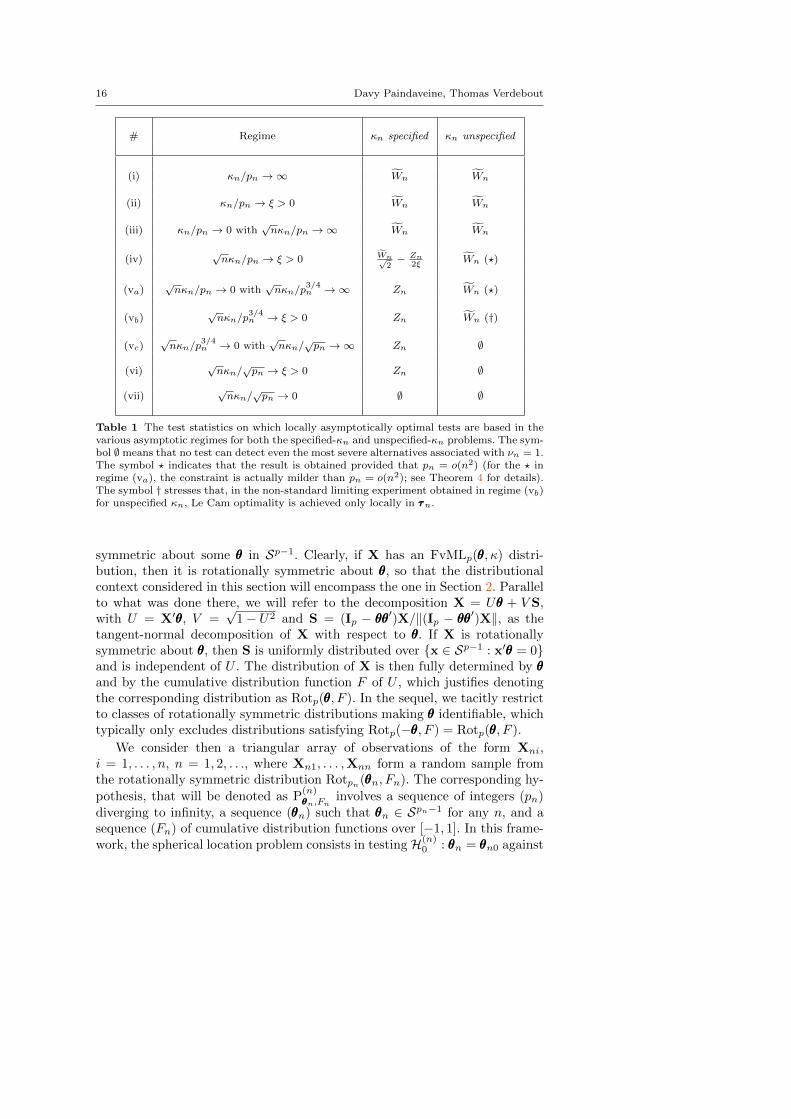
Wrapping up, we proved that the Watson test is optimal in regimes (i)–(iii) only for the specified concentration problem and that it is optimal in allregimes in the more important unspecified concentration one (in regimes (iv)–(va), optimality requires a constraint on pn that is at most pn = o(n2), andoptimality is only local in τττn in regime (vb)). The asymptotic cost due tothe unspecification of the concentration is nil in regimes (i)–(iii) (and (vii)),affects limiting powers but not consistency rates in regime (iv), and is in termsof consistency rates in regimes (v)–(vi). Table 1 provides a summary of theoptimality results we obtained both for the specified-κn and unspecified-κnproblems.

3 Non-null investigation via martingale CLTs

The results above thoroughly describe the asymptotic non-null and optimalityproperties of the Watson test in the FvML case and provide a strong motiva-tion to use this test in this specific parametric framework. While the Watsontest remains valid (in the sense that it still meets the asymptotic nominal levelconstraint) under much broader distributional assumptions, it is unclear howwell this test behaves under high-dimensional non-FvML alternatives (we re-fer to [30], [31] and [32] for an extensive study of the low-dimensional case).In this section, we therefore investigate, through a different approach relyingon martingale CLTs, the non-null behavior of the Watson test under generalrotationally symmetric distributions.

Recall that the distribution of a random vector X with values in Sp−1 is ro-tationally symmetric about θθθ(∈ Sp−1) if OX and X share the same distributionfor any O ∈ SOθθθ(p), and that it is rotationally symmetric if it is rotationally


# Regime κn specified κn unspecified

(i) κn/pn →∞ Wn Wn

(ii) κn/pn → ξ > 0 Wn Wn

(iii) κn/pn → 0 with√nκn/pn →∞ Wn Wn

(iv)√nκn/pn → ξ > 0 Wn√

2− Zn

2ξWn (?)

(va)√nκn/pn → 0 with

√nκn/p

3/4n →∞ Zn Wn (?)

(vb)√nκn/p

3/4n → ξ > 0 Zn Wn (†)

(vc)√nκn/p

3/4n → 0 with

√nκn/

√pn →∞ Zn ∅

(vi)√nκn/

√pn → ξ > 0 Zn ∅

(vii)√nκn/

√pn → 0 ∅ ∅

Table 1 The test statistics on which locally asymptotically optimal tests are based in thevarious asymptotic regimes for both the specified-κn and unspecified-κn problems. The sym-bol ∅ means that no test can detect even the most severe alternatives associated with νn = 1.The symbol ? indicates that the result is obtained provided that pn = o(n2) (for the ? inregime (va), the constraint is actually milder than pn = o(n2); see Theorem 4 for details).The symbol † stresses that, in the non-standard limiting experiment obtained in regime (vb)for unspecified κn, Le Cam optimality is achieved only locally in τττn.

symmetric about some θθθ in Sp−1. Clearly, if X has an FvMLp(θθθ, κ) distri-bution, then it is rotationally symmetric about θθθ, so that the distributionalcontext considered in this section will encompass the one in Section 2. Parallelto what was done there, we will refer to the decomposition X = Uθθθ + V S,with U = X′θθθ, V =

√1− U2 and S = (Ip − θθθθθθ′)X/‖(Ip − θθθθθθ′)X‖, as the

tangent-normal decomposition of X with respect to θθθ. If X is rotationallysymmetric about θθθ, then S is uniformly distributed over {x ∈ Sp−1 : x′θθθ = 0}and is independent of U . The distribution of X is then fully determined by θθθand by the cumulative distribution function F of U , which justifies denotingthe corresponding distribution as Rotp(θθθ, F ). In the sequel, we tacitly restrictto classes of rotationally symmetric distributions making θθθ identifiable, whichtypically only excludes distributions satisfying Rotp(−θθθ, F ) = Rotp(θθθ, F ).

We consider then a triangular array of observations of the form Xni,i = 1, . . . , n, n = 1, 2, . . ., where Xn1, . . . ,Xnn form a random sample fromthe rotationally symmetric distribution Rotpn(θθθn, Fn). The corresponding hy-

pothesis, that will be denoted as P(n)θθθn,Fn

involves a sequence of integers (pn)diverging to infinity, a sequence (θθθn) such that θθθn ∈ Spn−1 for any n, and asequence (Fn) of cumulative distribution functions over [−1, 1]. In this frame-work, the spherical location problem consists in testingH(n)

0 : θθθn = θθθn0 against


H(n)1 : θθθn 6= θθθn0, where (θθθn0) is a fixed null parameter sequence. Parallel to the

notation that was used in the FvML case, we will write en` and en`, ` = 1, 2, . . .for the non-central and central moments of Fn, respectively. These are themoments, under P

(n)θθθn,Fn

, of the quantity Un1 = X′n1θθθn in the tangent-normaldecomposition of Xn1 with respect to θθθn. The corresponding non-central mo-ments of Vn1 =

√1− U2

n1 will still be denoted as fn`.Using the notation Vni and Sni from the tangent-normal decomposition

of Xni with respect to the null location θθθn0, the Watson test statistic rewrites

Wn =Wn − (pn − 1)√

2(pn − 1)=

√2(pn − 1)∑ni=1 V

2ni

∑1≤i<j≤n

VniVnjS′niSnj ,

where Wn denotes the Watson test statistic in (1.2) based on the null loca-tion θθθn0. Under the null and under appropriate local alternatives, it is expectedthat Wn is asymptotically equivalent in probability to

W ∗n :=

√2(pn − 1)

nfn2

∑1≤i<j≤n

VniVnjS′niSnj ,

so that an important step in the investigation of the non-null properties of Wn

is the study of the non-null behavior of W ∗n . A classical martingale centrallimit theorem (see, e.g., Theorem 35.12 in [6]) provides the following result.

Theorem 5 Let (pn) be a sequence of integers that diverges to infinity and (θθθn0)be a sequence such that θθθn0 belongs to Spn−1 for any n. Let (Fn) be a se-quence of cumulative distribution functions on [−1, 1] such that (a) fn2 >0 for any n, (b) fn4/f

2n2 = o(n) and (c)

√pnen2 = o(1). Then, we have

the following, where, in each case, (τττn) refers to an arbitrary sequence suchthat θθθn = θθθn0+νnτττn belongs to Spn−1 for any n and such that (‖τττn‖) convergesto t(∈ [0,∞)) :

(i)–(iii) if (i)√nen1 → ∞, if (ii)

√nen1 → ξ > 0, or if (iii)

√nen1

→ 0 with√np

1/4n en1 →∞, then

W ∗nD−→ N

(t2√

2, 1

)under P

(n)θθθn0+νnτττn,Fn

, with νn =√fn2/(

√np

1/4n en1); in cases (i)–(ii), the

constraint (c) above is superfluous;

(iv) if√np

1/4n en1 → ξ > 0, then

W ∗nD−→ N

(ξ2t2√

2

(1− t2

4

), 1

)under P

(n)θθθn0+νnτττn,Fn

, with νn = 1;


(v) if√np

1/4n en1 = o(1), then

W ∗nD−→ N (0, 1)

under P(n)θθθn0+νnτττn,Fn

, with νn = 1.

To obtain the corresponding non-null results for the Watson test statis-tic Wn, we need to prove that Wn and W ∗n are indeed asymptotically equivalentin probability. The following result does so in the, possibly non-null, generalrotationally symmetric context considered (in the FvML case, the null versionof this result was established when proving the results of Section 2; see theproof of Lemma 2).

Theorem 6 Let (pn) be a sequence of integers that diverges to infinity and (θθθn0)be a sequence such that θθθn0 belongs to Spn−1 for any n. Let (Fn) be a sequenceof cumulative distribution functions on [−1, 1] such that (a) fn2 > 0 for any nand (b) fn4/f

2n2 = o(n). Then, with (νn) and (τττn) as in Theorem 5, we have

that, in each regime (i)–(v) considered there,

Wn = W ∗n + oP(1)

as n→∞ under P(n)θθθn0+νnτττn,Fn

.

Of course, Theorem 6 readily implies that Theorem 5 still holds if onesubstitutes Wn for W ∗n . Rather than restating the result explicitly, we presentthe following corollary, which focuses on the FvML case.

Corollary 1 Let (pn) be a sequence of integers that diverges to infinity, (κn)be a sequence in (0,∞), and (θθθn0) be a sequence such that θθθn0 belongs to Spn−1for any n. Then, we have the following, where in each case (τττn) refers to anarbitrary sequence such that θθθn = θθθn0 + νnτττn belongs to Spn−1 for any n andsuch that (‖τττn‖) converges to t(∈ [0,∞)) :

(i) if√nκn/p

3/4n →∞, then

W ∗nD−→ N

(t2√

2, 1

)under P


, with νn = p3/4n /(

√nκn√fn2 );

(ii) if√nκn/p

3/4n → ξ > 0, then

W ∗nD−→ N

(ξ2t2√

2

(1− t2

4

), 1

)under P


, with νn = 1;


(iii) if√nκn/p

3/4n = o(1), then

W ∗nD−→ N (0, 1)

under P(n)θθθn0+νnτττn,κn

, with νn = 1.

It is interesting to comment on how this relates to the results of the previoussection: Corollary 1(i) covers the regimes (i)–(iv) and (va). In view of theasymptotic behavior of fn2 in these regimes (see Lemma 4), Corollary 1(i)confirms the consistency rates of the Watson test in Theorem 2–4, as well asthe corresponding asymptotic powers obtained in (2.13) through the Le Camthird lemma. Corollary 1(ii) relates to regime (vb), where the Watson test canonly see the “fixed” alternatives associated with νn = 1, with limiting power

1− Φ(Φ−1(1− α)− ξ2t2√

2

(1− t2

4

))(3.19)

(note that this limiting power can be obtained both by using Corollary 1(ii)or by applying the Le Cam third lemma in Theorem 4, even if the secondapproach will provide the result only for alternatives associated with t <

√2,

that is, for alternatives in the open hemisphere centered at the null location).The limiting power in (3.19) increases monotonically from the nominal

level α (for t = 0, where the underlying location is the null one) to its maximalvalue (achieved at t =

√2, that is, when the true location is orthogonal to the

null one), then decreases monotonically to α (this limiting value being obtainedwhen the true location is antipodal to the null location). This non-monotonicpattern of the asymptotic power in this regime is a direct consequence of thenature of the Watson test that, as already mentioned, rejects the null when Xn

and θθθn0 project far from each other onto the orthogonal complement to θθθn0in Rpn . Finally, Corollary 1(iii) indicates that, for

√nκn/p

3/4n = o(1), there

are no alternatives under which the Watson test can show asymptotic powerslarger than the nominal level α, which is perfectly in line with results obtainedin the previous section for the corresponding regimes, namely for regimes (vc),(vi) and (vii).

4 Simulations

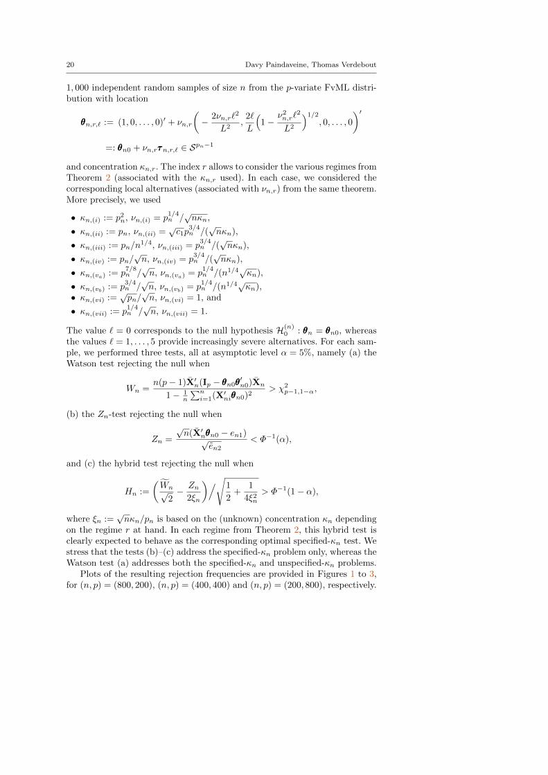
This section reports the results of a Monte Carlo study we conducted to seehow well the finite-sample behavior of the various tests reflect the asymp-totic findings in Theorems 2–4 and Corollary 1. To compare the results fordifferent values of p/n (note that most aforementioned asymptotic findingsallow pn to go to infinity at an arbitrary rate), we conducted three simu-lations, for (n, p) = (800, 200), (n, p) = (400, 400), and (n, p) = (200, 800),respectively. In each simulation, we generated, for every combination of r =(i), . . . , (iv), (va), (vb), (vi), (vii) and ` = 0, 1, . . . , L = 5, a collection of M =


1, 000 independent random samples of size n from the p-variate FvML distri-bution with location

θθθn,r,` := (1, 0, . . . , 0)′ + νn,r

(− 2νn,r`

2

L2,

2`

L

(1−

ν2n,r`2

L2

)1/2, 0, . . . , 0

)′=: θθθn0 + νn,rτττn,r,` ∈ Spn−1

and concentration κn,r. The index r allows to consider the various regimes fromTheorem 2 (associated with the κn,r used). In each case, we considered thecorresponding local alternatives (associated with νn,r) from the same theorem.More precisely, we used

• κn,(i) := p2n, νn,(i) = p1/4n /√nκn,

• κn,(ii) := pn, νn,(ii) =√c1p

3/4n /(

√nκn),

• κn,(iii) := pn/n1/4, νn,(iii) = p

3/4n /(

√nκn),

• κn,(iv) := pn/√n, νn,(iv) = p

3/4n /(

√nκn),

• κn,(va) := p7/8n /√n, νn,(va) = p

1/4n /(n1/4

√κn),

• κn,(vb) := p3/4n /√n, νn,(vb) = p

1/4n /(n1/4

√κn),

• κn,(vi) :=√pn/√n, νn,(vi) = 1, and

• κn,(vii) := p1/4n /√n, νn,(vii) = 1.

The value ` = 0 corresponds to the null hypothesis H(n)0 : θθθn = θθθn0, whereas

the values ` = 1, . . . , 5 provide increasingly severe alternatives. For each sam-ple, we performed three tests, all at asymptotic level α = 5%, namely (a) theWatson test rejecting the null when

Wn =n(p− 1)X′n(Ip − θθθn0θθθ′n0)Xn

1− 1n

∑ni=1(X′niθθθn0)2

> χ2p−1,1−α,

(b) the Zn-test rejecting the null when

Zn =

√n(X′nθθθn0 − en1)√

en2< Φ−1(α),

and (c) the hybrid test rejecting the null when

Hn :=

(Wn√

2− Zn

2ξn

)/√1

2+

1

4ξ2n> Φ−1(1− α),

where ξn :=√nκn/pn is based on the (unknown) concentration κn depending

on the regime r at hand. In each regime from Theorem 2, this hybrid test isclearly expected to behave as the corresponding optimal specified-κn test. Westress that the tests (b)–(c) address the specified-κn problem only, whereas theWatson test (a) addresses both the specified-κn and unspecified-κn problems.

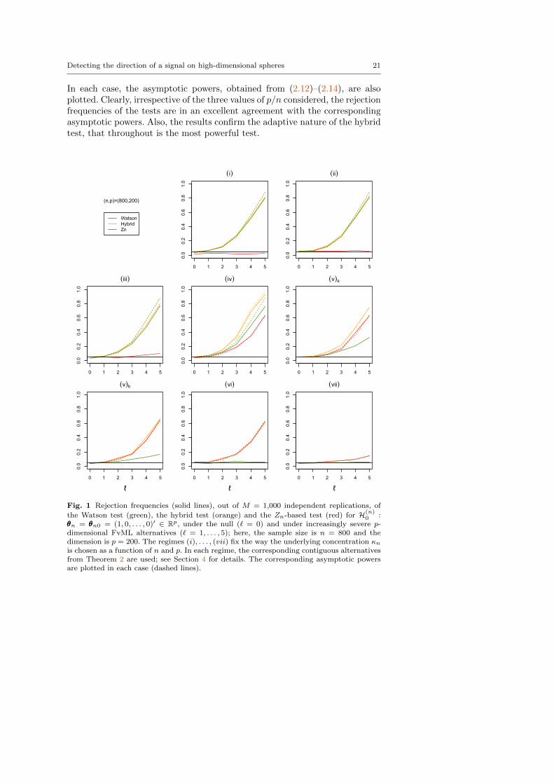
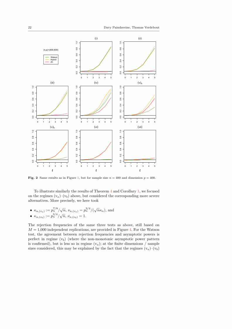
Plots of the resulting rejection frequencies are provided in Figures 1 to 3,for (n, p) = (800, 200), (n, p) = (400, 400) and (n, p) = (200, 800), respectively.


In each case, the asymptotic powers, obtained from (2.12)–(2.14), are alsoplotted. Clearly, irrespective of the three values of p/n considered, the rejectionfrequencies of the tests are in an excellent agreement with the correspondingasymptotic powers. Also, the results confirm the adaptive nature of the hybridtest, that throughout is the most powerful test.

WatsonHybridZn

(n,p)=(800,200)

0 1 2 3 4 5

0.0

0.2

0.4

0.6

0.8

1.0

(i)

0 1 2 3 4 5

0.0

0.2

0.4

0.6

0.8

1.0

(ii)

0 1 2 3 4 5

0.0

0.2

0.4

0.6

0.8

1.0

(iii)

0 1 2 3 4 5

0.0

0.2

0.4

0.6

0.8

1.0

(iv)

0 1 2 3 4 5

0.0

0.2

0.4

0.6

0.8

1.0

(v)a

0 1 2 3 4 5

0.0

0.2

0.4

0.6

0.8

1.0

(v)b

ℓ0 1 2 3 4 5

0.0

0.2

0.4

0.6

0.8

1.0

(vi)

ℓ0 1 2 3 4 5

0.0

0.2

0.4

0.6

0.8

1.0

(vii)

ℓ

Fig. 1 Rejection frequencies (solid lines), out of M = 1,000 independent replications, of

the Watson test (green), the hybrid test (orange) and the Zn-based test (red) for H(n)0 :

θθθn = θθθn0 = (1, 0, . . . , 0)′ ∈ Rp, under the null (` = 0) and under increasingly severe p-dimensional FvML alternatives (` = 1, . . . , 5); here, the sample size is n = 800 and thedimension is p = 200. The regimes (i), . . . , (vii) fix the way the underlying concentration κnis chosen as a function of n and p. In each regime, the corresponding contiguous alternativesfrom Theorem 2 are used; see Section 4 for details. The corresponding asymptotic powersare plotted in each case (dashed lines).


WatsonHybridZn

(n,p)=(400,400)

0 1 2 3 4 50.0

0.2

0.4

0.6

0.8

1.0

(i)

0 1 2 3 4 5

0.0

0.2

0.4

0.6

0.8

1.0

(ii)

0 1 2 3 4 5

0.0

0.2

0.4

0.6

0.8

1.0

(iii)

0 1 2 3 4 5

0.0

0.2

0.4

0.6

0.8

1.0

(iv)

0 1 2 3 4 50.0

0.2

0.4

0.6

0.8

1.0

(v)a

0 1 2 3 4 5

0.0

0.2

0.4

0.6

0.8

1.0

(v)b

ℓ0 1 2 3 4 5

0.0

0.2

0.4

0.6

0.8

1.0

(vi)

ℓ0 1 2 3 4 5

0.0

0.2

0.4

0.6

0.8

1.0

(vii)

ℓ

Fig. 2 Same results as in Figure 1, but for sample size n = 400 and dimension p = 400.

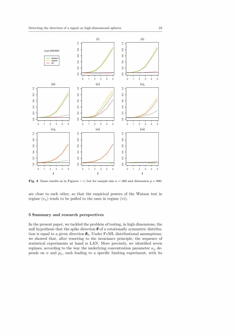
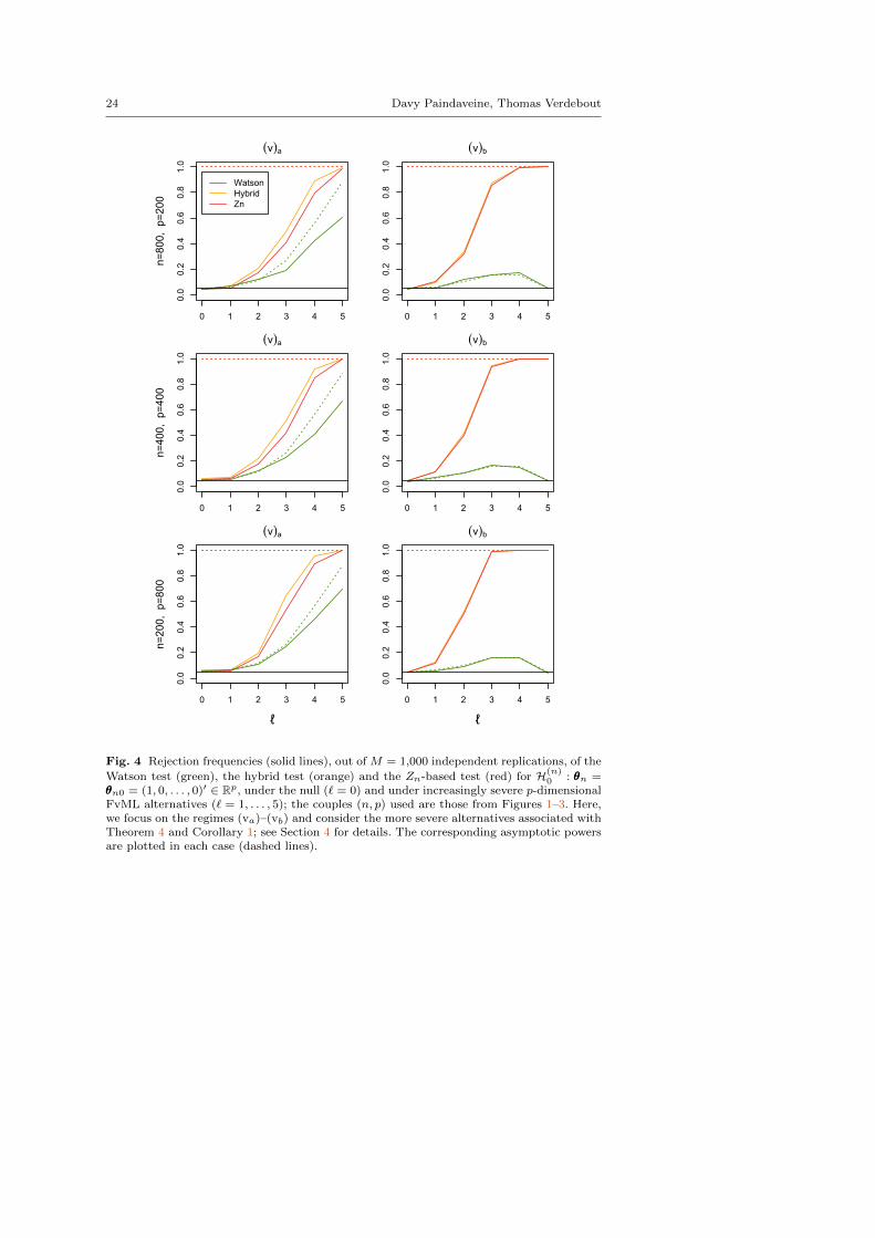
To illustrate similarly the results of Theorem 4 and Corollary 1, we focusedon the regimes (va)–(vb) above, but considered the corresponding more severealternatives. More precisely, we here took

• κn,(va) := p7/8n /√n, νn,(va) = p

3/4n /(

√nκn), and

• κn,(vb) := p3/4n /√n, νn,(vb) = 1.

The rejection frequencies of the same three tests as above, still based onM = 1,000 independent replications, are provided in Figure 4. For the Watsontest, the agreement between rejection frequencies and asymptotic powers isperfect in regime (vb) (where the non-monotonic asymptotic power patternis confirmed), but is less so in regime (va); at the finite dimensions / samplesizes considered, this may be explained by the fact that the regimes (va)–(vb)


WatsonHybridZn

(n,p)=(200,800)

0 1 2 3 4 50.0

0.2

0.4

0.6

0.8

1.0

(i)

0 1 2 3 4 5

0.0

0.2

0.4

0.6

0.8

1.0

(ii)

0 1 2 3 4 5

0.0

0.2

0.4

0.6

0.8

1.0

(iii)

0 1 2 3 4 5

0.0

0.2

0.4

0.6

0.8

1.0

(iv)

0 1 2 3 4 50.0

0.2

0.4

0.6

0.8

1.0

(v)a

0 1 2 3 4 5

0.0

0.2

0.4

0.6

0.8

1.0

(v)b

ℓ0 1 2 3 4 5

0.0

0.2

0.4

0.6

0.8

1.0

(vi)

ℓ0 1 2 3 4 5

0.0

0.2

0.4

0.6

0.8

1.0

(vii)

ℓ

Fig. 3 Same results as in Figures 1–2, but for sample size n = 200 and dimension p = 800.

are close to each other, so that the empirical powers of the Watson test inregime (va) tends to be pulled to the ones in regime (vi).

5 Summary and research perspectives

In the present paper, we tackled the problem of testing, in high dimensions, thenull hypothesis that the spike direction θθθ of a rotationally symmetric distribu-tion is equal to a given direction θθθ0. Under FvML distributional assumptions,we showed that, after resorting to the invariance principle, the sequence ofstatistical experiments at hand is LAN. More precisely, we identified sevenregimes, according to the way the underlying concentration parameter κn de-pends on n and pn, each leading to a specific limiting experiment, with its


0 1 2 3 4 5

0.0

0.2

0.4

0.6

0.8

1.0

n=80

0, p

=200

WatsonHybridZn

(v)a

0 1 2 3 4 5

0.0

0.2

0.4

0.6

0.8

1.0

(v)b

0 1 2 3 4 5

0.0

0.2

0.4

0.6

0.8

1.0

n=40

0, p

=400

(v)a

0 1 2 3 4 5

0.0

0.2

0.4

0.6

0.8

1.0

(v)b

0 1 2 3 4 5

0.0

0.2

0.4

0.6

0.8

1.0

n=20

0, p

=800

(v)a

ℓ0 1 2 3 4 5

0.0

0.2

0.4

0.6

0.8

1.0

(v)b

ℓ

Fig. 4 Rejection frequencies (solid lines), out of M = 1,000 independent replications, of the

Watson test (green), the hybrid test (orange) and the Zn-based test (red) for H(n)0 : θθθn =

θθθn0 = (1, 0, . . . , 0)′ ∈ Rp, under the null (` = 0) and under increasingly severe p-dimensionalFvML alternatives (` = 1, . . . , 5); the couples (n, p) used are those from Figures 1–3. Here,we focus on the regimes (va)–(vb) and consider the more severe alternatives associated withTheorem 4 and Corollary 1; see Section 4 for details. The corresponding asymptotic powersare plotted in each case (dashed lines).


own central sequence, Fisher information and contiguity rate (interestingly,these heterogeneous contiguity rates precisely quantify how difficult the prob-lem gets for low concentration situations). As a result, the Le Cam optimaltest (more precisely, the locally asymptotically most powerful invariant test)depends on the regime considered. In regimes where

√nκn/pn →∞, the clas-

sical Watson test is optimal, whereas in regimes where√nκn/pn = O(1), the

optimal test is an oracle test that explicitly involves the unknown value of theunderlying concentration κn. If

√nκn/pn → ξ > 0, then the Watson test fails

to be optimal but is still rate-consistent, whereas if√nκn/pn = o(1), then it

is not even rate-consistent. In all cases, we obtained from the Le Cam thirdLemma the asymptotic powers of the corresponding optimal tests and of theWatson test under contiguous alternatives. All results above allow the dimen-sion pn to go to infinity arbitrarily slowly or arbitrarily fast as a function of n,hence cover moderately high dimensions as well as ultra-high dimensions.

Optimality above refers to the specified-κn version of the testing problemconsidered. Since the concentration κn can hardly be assumed to be knownin practice, however, optimality results for the corresponding unspecified-κnproblem are more relevant. For this problem, the Watson test of course remainsoptimal in regimes where

√nκn/pn →∞. But remarkably, for unspecified κn,

the Watson test is also optimal in regimes where√nκn/pn = O(1), sometimes

under the condition that pn = o(n2) (on an even weaker condition on pn); werefer to Table 1 and to Theorems 3–4 for details.

Our work opens several perspectives for future research. (a) First, whilewe derived non-null results for the Watson test also outside the FvML dis-tributional setup, all our optimality results are limited to the FvML case. Anatural question is therefore whether or not the strong optimality propertiesof the Watson test extend away from the FvML case. The low-dimensionalinvestigation conducted in [31] leads us to conjecture that optimality wouldalso hold away from the FvML case, at least in low concentration patterns. Es-tablishing this would require expanding invariant log-likelihood ratios takinga much more complicated form than in the FvML case. This calls for entirelydifferent techniques, hence is beyond the scope of the present paper. (b) Sec-ond, we would like to mention that our results are also relevant in a Euclidean(i.e., non-directional) context. They indeed characterize the asymptotic effi-ciency of sign tests for the direction θθθ of a skewed single-spiked distributionin Rp, that is, a distribution whose projection along θθθ is skewed and whoseprojection onto the orthogonal complement to θθθ is spherically symmetric. Thisskewed version of the corresponding classical, elliptical, problem is natural ina signal detection framework, where the signal at hand is quite naturally max-imal in direction θθθ and minimal in the opposite direction −θθθ. While our resultsexhaustively address the question of efficiency of sign tests for this problem(that is, of tests that involve the observations only through their directionform the center of the distribution), it would be of interest to also considerthe efficiency of more general testing procedures.


A Technical proofs for Section 2

The proof of Theorem 1 requires the following preliminary results.

Lemma 1 Let (pn) be a sequence of integers diverging to infinity and (κn) be an arbitrarysequence in (0,∞). Let Ln :=

∑ni=1 V

2ni/(nfn2), where we used the notation Vni = (1 −

(X′niθθθn0)2)1/2 and fn2 = E[V 2n1]. Then, E

[(Ln − 1)2

]= o(p−1

n ) as n→∞ under P(n)θθθn0,κn

.

Proof of Lemma 1. Since

E

[(∑ni=1 V

2ni

nfn2− 1

)2]

=1

f2n2E

[(1

n

n∑i=1

V 2ni − E[V 2

n1]

)2]

=1

f2n2Var

[1

n

n∑i=1

V 2ni

]=

Var[V 2n1]

nf2n2=fn4 − f2n2nf2n2

(recall that fn4 := E[V 4n1]), it is sufficient to prove that

fn4 − f2n2f2n2

= O(p−1n ). (A.20)

Now, the expression for fn4/f2n2 in page 82 of [25] yields

∣∣∣∣fn4 − f2n2f2n2

∣∣∣∣ =

∣∣∣∣ (pn + 1)I pn2

+1(κn)I pn2−1(κn)

(pn − 1)(I pn2

(κn))2− 1

∣∣∣∣=

∣∣∣∣ (pn + 1)(I pn2

+1(κn)I pn2−1(κn)− (I pn

2(κn))2)

(pn − 1)(I pn2

(κn))2+

2

pn − 1

∣∣∣∣≤

3|I pn2

+1(κn)I pn2−1(κn)− (I pn

2(κn))2|

(I pn2

(κn))2+

2

pn − 1·

Since |I pn2

+1(κn)I pn2−1(κn)−(I pn

2(κn))2| ≤ (I pn

2(κn))2/( pn

2+1) (see (3.1)–(3.2) in [21]),

the result follows. �

Lemma 2 Let (pn) be a sequence of integers that diverges to infinity and (κn) be an arbi-trary sequence in (0,∞). Let (θθθn0) be a sequence such that θθθn0 belongs to Spn−1 for any n.

Consider the random variables Wn and Zn introduced in Theorem 1. Then, (Wn, Zn)′ is

asymptotically standard bivariate normal under P(n)θθθn0,κn

.

Proof of Lemma 2. Throughout the proof, expectations and variances are under P(n)θθθn0,κn

and stochastic convergences are as n→∞ under the same sequence of hypotheses, whereasUni, Vni and Sni refer to the tangent-normal decomposition of Xni with respect to θθθn0.Letting then

W ∗n =

√2(pn − 1)

nfn2

∑1≤i<j≤n

VniVnjS′niSnj ,


assume that (W ∗n , Zn)′ is asymptotically standard bivariate normal. Then,

Wn −W ∗n =

[√2(pn − 1)∑ni=1 V

2ni

−√

2(pn − 1)

nfn2

] ∑1≤i<j≤n

VniVnjS′niSnj (A.21)

=

[1−

∑ni=1 V

2ni

nfn2

]×

nfn2∑ni=1 V

2ni

×(√

2(pn − 1)

nfn2

∑1≤i<j≤n

VniVnjS′niSnj

)

=1− LnLn

W ∗n ,

where Ln was introduced in Lemma 1. This lemma implies that Ln − 1, hence also (1 −Ln)/Ln, is oP(1). If (W ∗n , Zn)′ is indeed asymptotically standard bivariate normal, then

we conclude that Wn − W ∗n is oP(1), so that (Wn, Zn)′ itself is asymptotically standardbivariate normal.

It is therefore sufficient to show that (W ∗n , Zn)′ is asymptotically standard bivariatenormal. We will do this by fixing γ and η such that γ2 + η2 = 1 and by using a classicalmartingale Central Limit Theorem to show that Dn := γW ∗n + ηZn is asymptotically stan-dard normal. To do so, let Fn` be the σ-algebra generated by Xn1, . . . ,Xn` and denote byEn`[.] the conditional expectation with respect to Fn`. Define Dn` := En`[Dn]−En,`−1[Dn]for ` = 1, . . . , n and Dn` = 0 for ` > n. It is then easy to check that Dn` = γW ∗n` + ηZn`,with

W ∗n` :=

√2(pn − 1)

nfn2

`−1∑i=1

VniVn`S′niSn` and Zn` :=

Un` − en1√nen2

for ` = 1, . . . , n and W ∗n` = 0 = Zn` for ` > n (W ∗n1 is also to be understood as zero). Toconclude from the martingale Central Limit Theorem in Theorem 35.12 from [6] that Dn =∑∞`=1Dn` is indeed asymptotically standard normal, we need to show that (a)

∑n`=1 σ

2n` →

1 in probability, with σ2n` := En,`−1[D2

n`], and that (b)∑n`=1 E[D2

n` I[|Dn`| > ε]] → 0 forany ε > 0. Clearly, for ` = 1, . . . , n,

σ2n` = γ2En,`−1[(W ∗n`)

2] + η2En,`−1[Z2n`] + 2γηEn,`−1[W ∗n`Zn`]

= γ2En,`−1[(W ∗n`)2] +

η2

n, (A.22)

so that (a) follows from Lemma A.1 in [25]. We may thus focus on (b). Since

En,`−1[(W ∗n`)2] = 2(n2fn2)−1

`−1∑i,j=1

VniVnjS′niSnj ,

we obtain Var[Dn`] = E[σ2n`] = γ2E[(W ∗n`)

2] + (η2/n) = 2γ2(` − 1)/n2 + (η2/n) ≤ 2/n,which yields that there exists a constant C such that, for any ε > 0,

n∑`=1

E[D2n` I[|Dn`| > ε]] ≤

n∑`=1

√E[D4

n`]√

P[|Dn`| > ε]

≤1

ε

n∑`=1

√E[D4

n`]√

Var[Dn`] ≤√

2√nε

n∑`=1

√E[D4

n`]

≤C√nε

n∑`=1

√E[(W ∗n`)

4] +C√nε

n∑`=1

√E[Z4

n`].


From (A.9) in [25], we then obtain

n∑`=1

E[D2n` I[|Dn`| > ε]] ≤

C√nε

n∑`=1

√12

n4

(`f2n4f4n2

+ `2fn4

f2n2

)+C√n

ε

√en4

n2e2n2

≤√

12C

ε

√( fn4

nf2n2

)2+

fn4

nf2n2+C

ε

√en4

ne2n2·

The result therefore follows from the fact that both fn4/f2n2 and en4/e2n2 are upper-boundedby a universal constant; see Theorem S.2.1 in [13]. �

Lemma 3 Let (νn) be a sequence in (0,∞) that diverges to ∞, (an), (bn) be sequencesin (0,∞) such that lim inf an > 0, bn/νn → ξ ∈ [0,∞) and b6n = o(a4nν

5n). Let Tn be a

sequence of random variables that is OP(1). Then, writing,

Hν(x) :=

∫ 1−1(1− t2)ν−

12 exp(xt) dt∫ 1

−1(1− t2)ν−12 dt

=Γ (ν + 1)Iν(x)

(x/2)ν,

we have that

a2n logHνn

( bnTnan

)=b2nT

2n

4νn−

b4nT4n

32ν3na2n

+ξ2T 2

n

4+ oP(1)

as n→∞.

Proof of Lemma 3. The proof is based on the bounds

Sν+ 12,ν+ 3

2(x) ≤ logHν(x) ≤ Sν,ν+2(x)

for any x > 0, with Sα,β(x) :=√x2 + β2 − β − α log((α +

√x2 + β2)/(α + β)); see (5) in

[20]. Consider

Gν(x) := logHν(x)−x2

4ν+

x4

32ν3+

x2

4ν2,

along with its resulting lower and upper bounds

Glowν (x) := Sν+ 1

2,ν+ 3

2(x)−

x2

4ν+

x4

32ν3+

x2

4ν2

and

Gupν (x) := Sν,ν+2(x)−

x2

4ν+

x4

32ν3+

x2

4ν2·

We prove the lemma by establishing that

a2nGlow/upνn

( bnTnan

)= oP(1). (A.23)

To do so, we expand the log term in Glow/upν (x) as log x = (x− 1)− 1

2(x− 1)2 + 1

3c3(x− 1)3

with c ∈ (1, x) (note that the argument of these log terms is larger than or equal to one),

and we write Glow/upν (x) = G

low/up,1ν (x) +G

low/up,2ν (x), with

Glow,1ν (x) :=

√x2 + (ν + 3

2)2 − (ν + 3

2)

−(ν + 12

)

[((ν + 1

2) +

√x2 + (ν + 3

2)2

2(ν + 1)− 1

)

−1

2

((ν + 1

2) +

√x2 + (ν + 3

2)2

2(ν + 1)− 1

)2]−x2

4ν+

x4

32ν3+

x2

4ν2,


Gup,1ν (x) :=

√x2 + (ν + 2)2 − (ν + 2)

−ν[(

ν +√x2 + (ν + 2)2

2(ν + 1)− 1

)

−1

2

(ν +

√x2 + (ν + 2)2

2(ν + 1)− 1

)2]−x2

4ν+

x4

32ν3+

x2

4ν2,

Glow,2ν (x) := −

ν + 12

3(clow)3

((ν + 1

2) +

√x2 + (ν + 3

2)2

2(ν + 1)− 1

)3

,

and

Gup,2ν (x) := −

ν

3(cup)3

(ν +

√x2 + (ν + 2)2

2(ν + 1)− 1

)3

.

Routine yet tedious computations allow to show that

Glow,1ν (x) =

x2

4ν2(ν + 1)+

(4ν2 + 5ν + 2)x4

32ν3(ν + 1)2(ν + 2)

+

(1−

4(1 + 2ν

)(1 + 32ν

)((1 + 3

2ν) +

√(xν

)2 + (1 + 32ν

)2)2)

x4

32(ν + 1)2(ν + 2)(A.24)

and

Gup,1ν (x) =

x2

4ν2(ν + 1)+

(4ν2 + 5ν + 2)x4

32ν3(ν + 1)2(ν + 2)

+

(1−

4(1 +

√( xν+2

)2 + 1)2)

x4

32(ν + 1)2(ν + 2)· (A.25)

Since both clow and cup are larger than one, we easily obtain

|Glow,2ν (x)| ≤

((1 + 3

2ν) +

√(xν

)2 + (1 + 32ν

)2)−3 (ν + 1

2)x6

24ν3(ν + 1)3(A.26)

and

|Gup,2ν (x)| ≤

((1 + 2

ν) +

√(xν

)2 + (1 + 2ν

)2)−3 x6

24ν2(ν + 1)3· (A.27)

Using the mean value theorem to control the last term in the righthand sides of (A.24)–(A.25), it directly follows from (A.24)–(A.27) that, under the assumptions of the lemma,

a2nGlow/up,1νn

( bnTnan

)= oP(1) and a2nG

low/up,2νn

( bnTnan

)= oP(1),

which proves (A.23), hence establishes the result. �

Proof of Theorem 1. Throughout the proof, distributions and expectations are un-

der P(n)θθθn0,κn

and stochastic convergences are as n → ∞ under the same sequence of hy-

potheses. By using the fact that Oθθθn0 = θθθn0 = O′θθθn0 for any O ∈ SOpn (θθθn0) and by


decomposing τττn into (τττ ′nθθθn0)θθθn0 +Πθθθn0τττn, with Πθθθn0

:= Ipn − θθθn0θθθ′n0, (2.7) yields

dP(n)Tn1− 1

2ν2n‖τττn‖2,κn

dmn=cnpn,κnωnpn−1

∫SOpn (θθθn0)

exp(nκnX

′nO′(θθθn0 + νnτττn)

)dO

=cnpn,κnωnpn−1

exp(nκnX

′nθθθn0

) ∫SOpn (θθθn0)

exp(nκnνnX

′nO′τττn)dO

=cnpn,κnωnpn−1

exp(nκnX

′nθθθn0


exp(nκnνnX

′n[(τττ ′nθθθn0)θθθn0 + O′Πθθθn0

τττn])dO

=cnpn,κnωnpn−1

exp(nκn(1 + νn(τττ ′nθθθn0))X′nθθθn0


exp(nκnνnX

′nO′Πθθθn0

τττn)dO.

Now, since O′Πθθθn0= O′Π2

θθθn0= Πθθθn0

O′Πθθθn0,∫

SOpn (θθθn0)exp

(nκnνnX

′nO′Πθθθn0

τττn)dO

=

∫SOpn (θθθn0)

exp(nκnνnX

′nΠθθθn0

O′Πθθθn0τττn)dO

=

∫SOpn (θθθn0)

exp

(nκnνn‖Πθθθn0

τττn‖‖Πθθθn0Xn‖

(Πθθθn0

Xn

‖Πθθθn0Xn‖

)′(O′

Πθθθn0τττn

‖Πθθθn0τττn‖

))dO

= E[

exp(nκnνn‖Πθθθn0

τττn‖‖Πθθθn0Xn‖v′nS

)|Xn1, . . . ,Xnn

],

where S is uniformly distributed over Spn−1θθθn0

:= {x ∈ Spn−1 : x′θθθn0 = 0} and where vn ∈

Spn−1θθθn0

is arbitrary. Since v′nS has density t 7→ cpn−1(1−t2)pn−4

2 I[t ∈ [−1, 1]], with cpn−1 =

1/∫ 1−1(1− t2)

pn−42 dt, this yields∫

SOpn (θθθn0)exp

(nκnνnX

′nO′Πθθθn0

τττn)dO

= cpn−1

∫ 1

−1exp(nκnνn‖Πθθθn0

τττn‖‖Πθθθn0Xn‖t

)(1− t2)

pn−42 dt

= H pn−32

(nκnνn‖Πθθθn0τττn‖‖Πθθθn0

Xn‖).

Summing up,

dP(n)Tn1− 1


dmn=cnpn,κnωnpn−1

exp(nκnX

′nθθθn0

)× exp

(nκnνn(τττ ′nθθθn0)X′nθθθn0

)H pn−3

2(nκnνn‖Πθθθn0

τττn‖‖Πθθθn0Xn‖). (A.28)

Now, with the quantity Ln introduced in Lemma 1, we have

Tn := 1 +

√2 Wn√pn − 1

=Wn

pn − 1=

n2∑ni=1 V

2ni

X′n(Ipn − θθθn0θθθ′n0)Xn

=n

fn2Ln‖Πθθθn0

Xn‖2 =nκn

(pn − 1)en1Ln‖Πθθθn0

Xn‖2,


where we used the identity fn2 = (pn − 1)en1/κn; see (2.9). Therefore, (A.28) yields


= log

dP(n)Tn1− 1


dP(n)Tn1,κn

= nκnνn(τττ ′nθθθn0)X′nθθθn0 + logH pn−32

(nκnνn‖Πθθθn0τττn‖‖Πθθθn0

Xn‖)

= nκnνn(τττ ′nθθθn0)X′nθθθn0 + logH pn−32

(n1/2(pn − 1)1/2κ1/2n νne

1/2n1 ‖Πθθθn0

τττn‖L1/2n T

1/2n ).

Since Wn =√

(pn − 1)/2× (Tn−1) is asymptotically standard normal (Lemma 2), we havethat Tn = 1 + oP(1). Moreover, it directly follows from Lemma 1 that Ln = 1 + oP(1).Consequently, Lemma 3 shows that, if νn satisfies (2.10), then


= nκnνn(τττ ′nθθθn0)X′nθθθn0 +pn − 1

2(pn − 3)nκnν

2nen1‖Πθθθn0

τττn‖2LnTn

−(pn − 1)2

4(pn − 3)3n2κ2nν

4ne

2n1‖Πθθθn0

τττn‖4L2nT

2n + oP(1).

Using (2.10), Lemma 1 and the fact that Tn = 1 + oP(1) yields


= nκnνn(τττ ′nθθθn0)X′nθθθn0 +1

2nκnν

2nen1‖Πθθθn0

τττn‖2Tn (A.29)

−n2κ2nν

4ne

2n1

4pn‖Πθθθn0

τττn‖4 + oP(1).

Using the definitions of Zn and Tn, we obtain


= nκnνn(τττ ′nθθθn0)(en1 +

√en2

n1/2Zn)

+1

2nκnν

2nen1‖Πθθθn0

τττn‖2(

1 +

√2 Wn√pn − 1

)−n2κ2nν

4ne

2n1

4pn‖Πθθθn0

τττn‖4 + oP(1)

=√nκnνn

√en2(τττ ′nθθθn0)Zn +

nκnν2nen1√2(pn − 1)1/2

‖Πθθθn0τττn‖2Wn

+nκnνn(τττ ′nθθθn0)en1 +1

2nκnν

2nen1‖Πθθθn0

τττn‖2 −n2κ2nν

4ne

2n1

4pn‖Πθθθn0

τττn‖4 + oP(1).

Using the identities

τττ ′nθθθn0 = −1

2νn‖τττn‖2 (A.30)

and

‖Πθθθn0τττn‖2 = ‖τττn‖2 − (τττ ′nθθθn0)2 = ‖τττn‖2

(1−

1

4ν2n‖τττn‖2

)(A.31)

provides


= −1

2

√nκnν

2n

√en2‖τττn‖2Zn

+nκnν2nen1√2(pn − 1)1/2

‖τττn‖2(

1−1

4ν2n‖τττn‖2

)Wn −

1

2nκnν

2nen1‖τττn‖2

+1

2nκnν

2nen1‖τττn‖2

(1−

1

4ν2n‖τττn‖2

)−n2κ2nν

4ne

2n1

4pn‖τττn‖4

(1−

1

4ν2n‖τττn‖2

)2+ oP(1).

The result then follows from (2.10) and from the tightness of Wn (Lemma 2). �


Lemma 4 Let (pn) be a sequence of integers that diverges to infinity and (κn) be anarbitrary sequence in (0,∞). Let en1 (resp., en2) be the expectation (resp., the variance)of the distribution with probability density function (2.8). Then, we have the following: (i)if κn/pn →∞, then

en1 = 1 + o(1), en2 = O( pnκ2n

)and fn2 =

pn

κn+ o( pnκn

);

(ii) if κn/pn → ξ > 0, then, letting cξ := 12

+√

14

+ ξ2,

en1 →ξ

cξ+ o(1), en2 = O

( 1

pn

)and fn2 =

1

cξ+ o(1);

(iii) if κn/pn → 0, then

en1 =κn

pn+O

(κ3np3n

), en2 =

1

pn+ o( 1

pn

)and fn2 = 1 + o(1).

Proof of Lemma 4. Denoting again as Iν(·) the order-ν modified Bessel function ofthe first kind, we recall (see (2.9)) that

en1 =I pn

2(κn)

I pn2−1(κn)

, en2 = 1−pn − 1

κnen1 − e2n1 and fn2 =

pn − 1

κnen1.

In each case (i)–(iii), the claim for fn2 directly follows from the result on en1, so that it issufficient to prove the results for en1 and en2. To do so, we will use the bounds

Rlowν (z) :=

z

ν + 1 +√

(ν + 1)2 + z2≤Iν+1(z)

Iν(z)≤

z

ν +√

(ν + 2)2 + z2=: Rup

ν (z) (A.32)

and

Rlowν (z) :=

z

ν + 12

+√

(ν + 32

)2 + z2≤Iν+1(z)

Iν(z); (A.33)

see (11) and (16) in [1], respectively. (i) The lower bound in (A.32) provides

en1 ≥κn

pn2

+√( pn

2

)2+ κ2n

=1

pn2κn

+√( pn

2κn

)2+ 1

,

which, since en1 ≤ 1, establishes the result for en1. Making use of the bound in (A.33), wecan write

en2 ≤ 1−pn − 1

κnRlowpn2−1

(κn)−(Rlowpn2−1

(κn))2.

Lengthy yet quite straightforward computations allow to rewrite this as

en2 ≤pn

κ2n

(pn−12κn

+√( pn+1

2κn

)2+ 1

)2 ·It readily follows that κ2nen2/pn is O(1), as was to be showed. Let us turn to the proofof (iii). The bounds in (A.32) readily yield

1

12

+√(

12

)2+(κnpn

)2 ≤ en1

κn/pn≤

1

12− 1pn

+√(

12

+ 1pn

)2+(κnpn

)2 , (A.34)

which provides

−(κnpn

)2(12

+√(

12

)2+(κnpn

)2)2 ≤ en1

κn/pn− 1 ≤

−(κnpn

)212− 1pn

+√(

12

+ 1pn

)2+(κnpn

)2 ·


This proves the result for en1. Turning to en2, the bounds in (A.32) lead to

1−pn − 1

κnRuppn2−1

(κn)−(Ruppn2−1

(κn))2 ≤ en2 ≤ 1−

pn − 1

κnRlowpn2−1

(κn)−(Rlowpn2−1

(κn))2.

As above, heavy but rather straightforward computations allow to rewrite this as

32

+ 1pn−√(

12

+ 1pn

)2+(κnpn

)2pn(

12− 1pn

+√(

12

+ 1pn

)2+(κnpn

)2 )2 ≤ en2 ≤ 1

pn(

12

+√(

12

)2+(κnpn

)2 ) , (A.35)

which establishes that pnen2 = 1+o(1). Finally, the result in (ii) readily follows from (A.34)and from the upper bound in (A.35). �

Proof of Theorem 2. Stochastic convergences throughout the proof are as n → ∞under P

(n)θθθn0,κn

. Assume that (i) κn/pn → ∞, (ii) κn/pn → ξ > 0, or (iii) κn/pn → 0

with√nκn/pn → ∞, and let (νn) be the corresponding sequence in the statement of

the theorem. Using Lemma 4 and the identity κnfn2 = (pn − 1)en1, it is then easy tocheck that νn satisfies (2.10), is such that νn = o(1), and is asymptotically equivalent to

νn = p3/4n /(

√nκn√fn2) in the sense that νn/νn → 1. Theorem 1 thus applies and yields


= −p3/2n√en2

2√nκnfn2

‖τττn‖2Zn +pnen1√2κnfn2

‖τττn‖2Wn

−p3nen1

8nκ3nf2n2

‖τττn‖4 −p2ne

2n1

4κ2nf2n2

‖τττn‖4 + oP(1).

Using again the identity κnfn2 = (pn − 1)en1, we then obtain


= −p3/2n√en2

2√n(pn − 1)en1

‖τττn‖2Zn +1√

2‖τττn‖2Wn (A.36)

−p3n

8nκn(pn − 1)2en1‖τττn‖4 −

1

4‖τττn‖4 + oP(1).

The result in cases (i)–(iii) then follows from the fact that Lemma 4 implies that, in eachcase, the first and third term of the righthand side of (A.36) are oP(1).

We turn to case (iv), for which√nκn/pn = ξ (so that, like for all subsequent cases, κn =

o(pn)). Then, the same argument as above allows to check that νn = p3/4n /(

√nκn√fn2)

still satisfies (2.10) and is such that νn = o(1), so that, jointly with Lemma 4, Theorem 1provides


= −p3/2n e

1/2n2

2√nκnfn2

‖τττn‖2Zn +pnen1√2κnfn2

‖τττn‖2Wn

−p3nen1

8nκ3nf2n2

‖τττn‖4 −p2ne

2n1

4κ2nf2n2

‖τττn‖4 + oP(1)

= −1

2ξ‖τττn‖2Zn +

1√

2‖τττn‖2Wn −

1

8ξ2‖τττn‖4 −

1

4‖τττn‖4 + oP(1),

as was to be shown. Consider now case (v), under which√nκn/pn → 0 with

√nκn/

√pn →

∞, which still ensures that νn = p1/4n /(n1/4√κn) is o(1) and satisfies (2.10). Theorem 1

applies and, by using Lemma 4 again, yields


= −1

2

√pnen2 ‖τττn‖2Zn +

√nen1√

2‖τττn‖2Wn −

pnen1

8κn‖τττn‖4 −

ne2n14‖τττn‖4 + oP(1)

= −1

2‖τττn‖2Zn −

1

8‖τττn‖4 + oP(1),


which establishes the result in case (v). If√nκn/

√pn = ξ (case (vi)), then Lemma 4 implies

that νn = 1 satisfies (2.10). Theorem 1 then provides


= −√nκn

2√pn

√pnen2 ‖τττn‖2Zn +

nκnen1√

2p1/2n

‖τττn‖2(

1−1

4‖τττn‖2

)Wn

−1

8nκnen1‖τττn‖4 −

n2κ2ne2n1

4pn‖τττn‖4

(1−

1

4‖τττn‖2

)2+ oP(1) (A.37)

= −ξ

2‖τττn‖2Zn −

ξ2

8‖τττn‖4 + oP(1),

where we used Lemma 4. Finally, if√nκn/

√pn = o(1) (case (vii)), then (2.10) again holds

for νn = 1. Therefore, Theorem 1 shows that Λ(n)invθθθn/θθθn0;κn

satisfies the first equality of (A.37),

hence is oP(1). �

Proof of Theorem 3. First note that, since pn = o(n2), Lemma 4(iii) entails that

Zn =

√n(X′nθθθn0 − en1)√e2n

=

√n(X′nθθθn0 − ξ/

√n+O(n−3/2))√

1pn

+ o( 1pn

)

=

√pn(√nX′nθθθn0 − ξ +O(1/n))√

1 + o(1)=√npnX

′nθθθn0 −

√pnξ + oP(1) (A.38)


. Write then


= Λ(n)invθθθn,κn,s/θθθn0,κn,s

+ Λ(n)invθθθn0,κn,s/θθθn0,κn

= Λ(n)invθθθn,κn,s/θθθn0,κn,s

+ logdP

(n)θθθn0,κn,s

dP(n)θθθn0,κn

=: Ln1 + Ln2.

Using (A.38), we obtain

Ln2 = n(

log(cpn,κn,s )− log(cpn,κn ))

+ n(κn,s − κn)X′nθθθn0

= n[

log( cpn,0

cpn,κn

)− log

( cpn,0

cpn,κn,s

)]+ s√npn X′nθθθn0

= n[

logH pn2−1(κn)− logH pn

2−1(κn,s)

]+ s√pnξ + sZn + oP(1)

=: Ln2 + sZn + oP(1)


. Since pn = o(n2), we can apply Lemma 3 with an =√n and

Tn ≡ 1. This yields

Ln2 =( nκ2n

4( pn2− 1)

−nκ4n

32( pn2− 1)3

)−( nκ2n,s

4( pn2− 1)

−nκ4n,s

32( pn2− 1)3

)+ s√pnξ + o(1)

= −n(κ2n,s − κ2n)

2pn − 4+n(κ4n,s − κ4n)

4(pn − 2)3+ s√pnξ + o(1)

= −p2n((ξ + s/

√pn)2 − ξ2)

2pn − 4+p4n((ξ + s/

√pn)4 − ξ4)

4n(pn − 2)3+ s√pnξ + o(1)

= −s2

2+ o(1)


as n→∞. Therefore,

Ln2 = sZn −s2

2+ oP(1) (A.39)


, which implies that the sequences of probability measures P(n)θθθn0,κn,s

and P(n)θθθn0,κn

are mutually contiguous (this results from the Le Cam first lemma).

Now, denote as en1,s and e2n,s, respectively, the values of en1 and e2n under P(n)θθθn0,κn,s

.

Then, proceeding as in (A.38) and using the fact that contiguity implies that (A.38) also

holds under P(n)θθθn0,κn,s

, one obtains

Zn,s :=

√n(X′nθθθn0 − en1,s)√

e2n,s=√npnX

′nθθθn0 −

√pnξ − s+ oP(1) = Zn − s+ oP(1)

as n→∞ under P(n)θθθn0,κn,s

. Consequently, Theorem 2(iv) implies that

L1n=‖τττn‖2(Wn√

2−Zn,s

2ξ

)−

1

2‖τττn‖4

(1

2+

1

4ξ2

)+ oP(1)

=‖τττn‖2(Wn√

2−Zn

2ξ

)+‖τττn‖2s

2ξ−

1

2‖τττn‖4

(1

2+

1

4ξ2

)+ oP(1) (A.40)

as n → ∞ under P(n)θθθn0,κn,s

, hence, from contiguity, also under P(n)θθθn0,κn

. Combining (A.44)

and (A.40) establishes the local asymptotic quadraticity result in (2.18). Finally, the asymp-totic normality result of ∆∆∆n trivially follows from Lemma 2. �

The proof of Theorem 4 requires both following lemmas.

Lemma 5 Let (pn) be a sequence of integers that diverges to infinity. Let (κn) and (κn∗)be sequences in (0,∞) that are o(pn) and write en1 and en2 (resp., en1∗ and en2∗) for thecorresponding moments based on κn (resp., on κn∗). Let (θθθn0), (νn) and (τττn) be sequencessuch that θθθn0 and θθθn = θθθn0 +νnτττn belong to Spn−1 for any n, with (τττn) bounded and (νn)such that

ν2n = O( √

pn

nκn∗en1∗

). (A.41)

Then, with the same Zn and Wn as in Theorem 1, we have that

Λ(n)invθθθn/θθθn0;κn∗

= −1

2

√nκn∗ν

2n

√en2 ‖τττn‖2Zn +

nκn∗ν2nen1∗√2p

1/2n

‖τττn‖2(

1−1

4ν2n‖τττn‖2

)Wn

−1

8nκn∗ν

4nen1∗‖τττn‖4 −

n2κ2n∗ν4ne

2n1∗

4pn‖τττn‖4

(1−

1

4ν2n‖τττn‖2

)2+

1

2nκn∗ν

2n(en1∗ − en1)‖τττn‖2 + oP(1),


.

Proof of Lemma 5. Since κn and κn∗ are both o(n), Lemma 4 ensures that fn2/fn2∗ =1+o(1), where fn2∗ denotes the quantity fn2 based on κn∗. Using this, it can be showed along

the exact same lines as in the proof of (A.29) in Theorem 1 that, as n→∞ under P(n)θθθn0,κn

,

Λ(n)invθθθn/θθθn0;κn∗

= nκn∗νn(τττ ′nθθθn0)X′nθθθn0 +1

2nκn∗ν

2nen1∗‖Πθθθn0

τττn‖2Tn

−n2κ2n∗ν

4ne

2n1∗

4pn‖Πθθθn0

τττn‖4 + oP(1),


where Tn := 1+√

2 Wn/√pn − 1. If one replaces Tn by this expression and X′nθθθn0 by en1 +√

en2Zn/√n, then the result follows by using (A.30), (A.31), (A.41), and the tightness

of Wn. �

The second lemma reinforces the variance result in Lemma 4(iii).

Lemma 6 Let (pn) be a sequence of integers that diverges to infinity and (κn) be a sequencein (0,∞) that is o(pn). Denote as en2 the variance of the distribution with probability densityfunction (2.8). Then,

√pnen2 − 1 = O(κ2n/p

2n) as n→∞.

Proof of Lemma 6. In this proof, C denotes a generic constant that may differ fromline to line. Since (A.35) yields√

32

+ 1pn−√(

12

+ 1pn

)2+(κnpn

)212− 1pn

+√(

12

+ 1pn

)2+(κnpn

)2 − 1 ≤√pnen2 − 1 ≤

1√12

+√(

12

)2+(κnpn

)2 − 1 ≤ 0,

we have

|√pnen2 − 1| ≤ 1−

√32

+ 1pn−√(

12

+ 1pn

)2+(κnpn

)212− 1pn

+√(

12

+ 1pn

)2+(κnpn

)2≤ C

{(12− 1pn

+√(

12

+ 1pn

)2+(κnpn

)2)−√ 32

+ 1pn−√(

12

+ 1pn

)2+(κnpn

)2 }

≤ C{(

12− 1pn

+√(

12

+ 1pn

)2+(κnpn

)2)2 − ( 32

+ 1pn−√(

12

+ 1pn

)2+(κnpn

)2)}.

Standard computations allow us to rewrite this upper-bound as

|√pnen2 − 1| ≤ C

{2(pn−1)pn

√( pn+22pn

)2+(κnpn

)2 − (pn−1)(pn+2)−κ2n

p2n

}

≤ C{

4(pn−1)2

p2n

(( pn+22pn

)2+(κnpn

)2)− ((pn−1)(pn+2)−κ2n)

2

p4n

}= C

(6− 6

pn− κ2

np2n

)κ2np2n·

which, for n large, is upper-bounded by Cκ2n/p2n, as was to be proved. �

Proof of Theorem 4. Since κn = o(pn), Lemma 4(iii) entails that

Zn =

√n(X′nθθθn0 − en1)√e2n

=

√n(X′nθθθn0 − ξrn/

√n+O(r3nn

−3/2))√1pn

+ o( 1pn

)

=

√pn(√nX′nθθθn0 − ξrn +O(r3nn

−1))√1 + o(1)

=√npnX

′nθθθn0 − ξ

√pnrn +OP

(√pnr3nn

)(A.42)


. Write then


= Λ(n)invθθθn,κn,s,τττn/θθθn0,κn,s,τττn

+ Λ(n)invθθθn0,κn,s,τττn/θθθn0,κn

= Λ(n)invθθθn,κn,s,τττn/θθθn0,κn,s,τττn

+ logdP

(n)θθθn0,κn,s,τττn

dP(n)θθθn0,κn

=: Ln1 + Ln2.


Letting ρn := (1− 12ν2n‖τττn‖2)−1 and using (A.42), we obtain

Ln2 = n(

log(cpn,κn,s,τττn )− log(cpn,κn ))

+ n(κn,s,τττn − κn)X′nθθθn0

= n[

log( cpn,0

cpn,κn

)− log

( cpn,0

cpn,κn,s,τττn

)]+ ρn(s

√npn + 1

2ξ√npnrnν

2n‖τττn‖2) X′nθθθn0

= n[


2−1(κn,s,τττn )

]+ρn(s

√npn + 1

2ξ√npnrnν

2n‖τττn‖2)

(Zn√npn

+ξrn√n

+OP

( r3nn3/2

))as n→∞ under P

(n)θθθn0,κn

. Since√pnr3n and pnr4nν

2n are o(n), this yields

Ln2 = n[


2−1(κn,s,τττn )

]+ρn

(s+ 1

2ξ√pnrnν

2n‖τττn‖2

)Zn + ξsρnrn

√pn + 1

2ξ2ρnpnr

2nν

2n‖τττn‖2 + oP(1)

=: Ln2 + ρn(s+ 12ξ√pnrnν

2n‖τττn‖2)Zn + oP(1)


. Since pn = o(n2r−4n ), we can apply Lemma 3 with an =

√n and

Tn ≡ 1, which provides

Ln2 =( nκ2n

4( pn2− 1)

−nκ4n

32( pn2− 1)3

)−( nκ2n,s,τττn

4( pn2− 1)

−nκ4n,s,τττn

32( pn2− 1)3

)+ξsρnrn

√pn + 1

2ξ2ρnpnr

2nν

2n‖τττn‖2 + o(1)

= −n(κ2n,s,τττn − κ

2n)

2pn − 4+n(κ4n,s,τττn − κ

4n)

4(pn − 2)3+ ξsρnrn

√pn + 1

2ξ2ρnpnr

2nν

2n‖τττn‖2 + o(1)

= −p2nr

2n{ρ2n(ξ + s/(

√pnrn))2 − ξ2}

2pn − 4+ Sn + ξsρnrn

√pn + 1

2ξ2ρnpnr

2nν

2n‖τττn‖2 + o(1),

where, since 1− ρn = − 12ρnν2n‖τττn‖2,

Sn =p4nr

4n{ρ4n(ξ + s/(

√pnrn))4 − ξ4}

4n(pn − 2)3=

p4nr4n

4n(pn − 2)3

((ρ4n − 1)ξ4 +

∑4`=1

(4`

) s`ξ4−`

(√pnrn)`

)

= O(pnr4n

n(ρn − 1)(ρn + 1)(ρ2n + 1)

)+O

(√pnr3nn

)= O

(pnr4nν2nn

)+O

(√pnr3nn

)= o(1).

Thus, using the identities 1− ρn = − 12ρnν2n‖τττn‖2 and ρ2n− 1 = ρ2nν

2n‖τττn‖2− 1

4ρ2nν

4n‖τττn‖4,

we have

Ln2 = −(ρ2n − 1)ξ2p2nr

2n

2pn − 4−s2ρ2npn

2pn − 4−

2ξsρ2np3/2n rn

2pn − 4+ ξsρnrn

√pn + 1

2ξ2ρnpnr

2nν

2n‖τττn‖2 + o(1)

= −1

2ξ2ρ2npnr

2nν

2n‖τττn‖2 +

1

8ξ2ρ2npnr

2nν

4n‖τττn‖4 −

1

2s2ρ2n (A.43)

−ξsρ2n√pnrn + ξsρnrn

√pn + 1

2ξ2ρnpnr

2nν

2n‖τττn‖2 + o(1)

=1

2ξ2ρn(1− ρn)pnr

2nν

2n‖τττn‖2 +

1

8ξ2ρ2npnr

2nν


1

2s2ρ2n + ξsρn(1− ρn)

√pnrn + o(1)

= −1

2s2ρ2n −

1

2ξsρ2n

√pnrnν


1

8ξ2ρ2npnr

2nν

4n‖τττn‖4 + o(1)


as n→∞. Therefore, we proved that, as n→∞ under P(n)θθθn0,κn

,

Ln2 = ρn(s+ 12ξ√pnrnν

2n‖τττn‖2)Zn (A.44)

−1

2s2ρ2n −

1

2ξsρ2n

√pnrnν


1

8ξ2ρ2npnr

2nν

4n‖τττn‖4 + oP(1).

We turn to L1n. Write cn,s,τττn := nν2nκn,s,τττnen1,s,τττn/√pn, where en1,s,τττn and e2n,s,τττn

denote the values of en1 and e2n under P(n)θθθn0,κn,s,τττn

. Since√pnr2nν

2n = O(1), (A.48) below

ensures that cn,s,τττn is O(1). Therefore, Lemma 5 yields

L1n = LZ1n + LZ1n + LZ1n + LW1n + oP(1), (A.45)

where we let

LZ1n := −1

2

√nκn,s,τττnν

2n

√en2 ‖τττn‖2Zn, LZ1n := −

1

8

√pnν

2ncn,s,τττn‖τττn‖4,

LZ1n :=1

2nκn,s,τττnν

2n(en1,s,τττn − en1)‖τττn‖2,

and

LW1n :=1√

2cn,s,τττn‖τττn‖2

(1−

1

4ν2n‖τττn‖2

)Wn −

1

4c2n,s,τττn‖τττn‖

4(

1−1

4ν2n‖τττn‖2

)2.

Lemma 6 provides

LZ1n = −√nν2n

2√pn‖τττn‖2

(ρnpnrn√n

(ξ +

s√pnrn

))√pen2 Zn

= −1

2ρn√pnrnν

2n‖τττn‖2

(ξ +

s√pnrn

)(1 +O

(κ2np2n

))Zn

= −1

2ξρn√pnrnν

2n‖τττn‖2Zn −

1

2sρnν

2n‖τττn‖2Zn + oP(1), (A.46)

where we used the fact that√pnr3nν

2n is o(n).

Now, Lemma 4(iii) yields

en1,s,τττn =κn,s,τττnpn

+O(κ3n,s,τττn

p3n

)=ρnrn√n

(ξ +

s√pnrn

)+O

( r3nn3/2

)

=ξρnrn√

n+

sρn√npn

+O( r3nn3/2

), (A.47)

so that

cn,s,τττn =nν2n√pn

(ρnpnrn√n

(ξ +

s√pnrn

))( ξρnrn√n

+sρn√npn

+O( r3nn3/2

))

= ρ2n√pnr

2nν

2n

(ξ +

s√pnrn

)(ξ +

s√pnrn

+O( r2nn

)), (A.48)

which in turn implies that

LZ1n = −1

8

√pnν

2n

(ξ2ρ2n

√pnr

2nν

2n + 2ξsρ2nrnν

2n + s2

ρ2nν2n√pn

+O(√pnr4nν2n

n

))‖τττn‖4

= −1

8ξ2ρ2npnr

2nν


1

4ξsρ2n

√pnrnν


1

8s2ρ2nν

4n‖τττn‖4 + o(1). (A.49)


Using (A.47) and applying Lemma 4(iii) again, we obtain

en1,s,τττn − en1 =

(ξρnrn√

n+

sρn√npn

+O( r3nn3/2

))−κn

pn+O

(κ3np3n

)

=ξ(ρn − 1)rn√

n+

sρn√npn

+O( r3nn3/2

)=ξρnrnν2n

2√n‖τττn‖2 +

sρn√npn

+O( r3nn3/2

),

so that

LZ1n =1

2n(ρnpnrn√

n

(ξ +

s√pnrn

))ν2n

(ξρnrnν2n


sρn√npn

+O( r3nn3/2

))‖τττn‖2

=1

2ρnpnrn

√nν2n‖τττn‖2ξ

(ξρnrnν2n


sρn√npn

+O( r3nn3/2

))

+1

2ρnpnrn

√nν2n‖τττn‖2

s√pnrn

(ξρnrnν2n


sρn√npn

+O( r3nn3/2

))

=1

4ξ2ρ2npnr

2nν

4n‖τττn‖4 +

1

2ξsρ2n

√pnrnν

2n‖τττn‖2

+1

4ξsρ2n

√pnrnν

4n‖τττn‖4 +

1

2s2ρ2nν

2n‖τττn‖2 + o(1), (A.50)

where we used the facts that pnr4nν2n and

√pnr3nν

2n are o(n).

Jointly with (A.44), (A.46), (A.49), and (A.50), this shows that


− LW1n = sρn(1− 12ν2n‖τττn‖2)Zn −

1

2s2ρ2n(1− ν2n‖τττn‖2 + 1

4ν4n‖τττn‖4) + oP(1)

= sZn −1

2s2 + oP(1).

The result thus follows from the definition of LW1n and the fact that (A.48) implies thatcn,s,τττn = 1 + o(1) in case (a), cn,s,τττn = ξ2 + o(1) in case (b), and cn,s,τττn = o(1) in case (c)(in each case, the asymptotic normality result of ∆∆∆n follows from Lemma 2). �

B Technical proofs for Section 3

The proof of Theorem 5 requires the following lemma.

Lemma 7 Let Mn := θθθnθθθ′n − θθθn0θθθ′n0, where (θθθn) and (θθθn0) belong to Spn−1. Then, for

any real numbers a, b, c, d, we have that tr[M`n(aθθθnθθθ

′n+b(Ipn−θθθnθθθ′n))M`

n(cθθθnθθθ′n+d(Ipn−

θθθnθθθ′n))]

is equal to (ad + bc)(1 − (θθθ′n0θθθn)2) + (a − b)(c − d)(1 − (θθθ′n0θθθn)2)2 for ` = 1 andto (ac+ bd)(1− (θθθ′n0θθθn)2)2 for ` = 2.

Proof of Lemma 7. Direct computations yield

M2n = θθθnθθθ

′n + θθθn0θθθ

′n0 − (θθθ′nθθθn0)θθθn0θθθ

′n − (θθθ′nθθθn0)θθθnθθθ

′n0 and M4

n = (1− (θθθ′n0θθθn)2)M2n.

This provides tr[M2n] = 2(1 − (θθθ′n0θθθn)2) and tr[M4

n] = 2(1 − (θθθ′n0θθθn)2)2, and allows toshow that θθθ′nM

2nθθθn = 1 − (θθθ′nθθθn0)2 and θθθ′nM

4nθθθn = (1 − (θθθ′n0θθθn)2)2. Since θθθ′nMnθθθn =


1− (θθθ′n0θθθn)2, this yields

tr[Mn(aθθθnθθθ

′n + b(Ipn − θθθnθθθ′n))Mn(cθθθnθθθ

′n + d(Ipn − θθθnθθθ′n))

]= tr

[Mn(bIpn + (a− b)θθθnθθθ′n)Mn(dIpn + (c− d)θθθnθθθ

′n)]

= bd tr[M2n] + b(c− d)θθθ′nM

2nθθθn + (a− b)dθθθ′nM2

nθθθn + (a− b)(c− d)(θθθ′nMnθθθn)2

= 2bdθθθ′nMnθθθn + {b(c− d) + (a− b)d}θθθ′nMnθθθn + (a− b)(c− d)(θθθ′nMnθθθn)2

= (ad+ bc)(1− (θθθ′n0θθθn)2) + (a− b)(c− d)(1− (θθθ′n0θθθn)2)2

and

tr[M2n(aθθθnθθθ

′n + b(Ipn − θθθnθθθ′n))Mn(cθθθnθθθ

′n + d(Ipn − θθθnθθθ′n))

]= tr

[M2n(bIpn + (a− b)θθθnθθθ′n)M2

n(dIpn + (c− d)θθθnθθθ′n)]

= bd tr[M4n] + b(c− d)θθθ′nM

4nθθθn + (a− b)dθθθ′nM4

nθθθn + (a− b)(c− d)(θθθ′nM2nθθθn)2

= 2bd(θθθ′nMnθθθn)2 + {b(c− d) + (a− b)d}(θθθ′nMnθθθn)2 + (a− b)(c− d)(θθθ′nMnθθθn)2

= {ad+ bc+ (a− b)(c− d)}(1− (θθθ′n0θθθn)2)2

= (ac+ bd)(1− (θθθ′n0θθθn)2)2,

as was to be showed. �

Proof of Theorem 5. All expectations and variances below are taken under P(n)θθθn,Fn

,

with θθθn = θθθn0 + νnτττn, and stochastic convergences are under the corresponding sequenceof hypotheses. We have

E[Xni] = en1θθθn and E[XniX′ni] = en2θθθnθθθ

′n +

fn2

pn − 1(Ipn − θθθnθθθ′n);

see the proof of Lemma B.3 in [12]. Writing Wni := (Ipn − θθθnθθθ′n)Xni, this implies that

E[Wni] = 0 and E[WniW′ni] =

fn2

pn − 1(Ipn − θθθnθθθ′n). (B.51)

Writing Mn = θθθnθθθ′n − θθθn0θθθ′n0 as in Lemma 7 and Yni := (Ipn − θθθn0θθθ′n0)Xni, we have

Wni = Yni −MnXni. This allows to decompose W ∗n as

W ∗n :=

√2(pn − 1)

nfn2

∑1≤i<j≤n

Y′niYnj

=

√2(pn − 1)

nfn2

∑1≤i<j≤n

(W′niWnj + X′niMnWnj + W′

niMnXnj + X′niM2nXnj)

=:W ∗n0 +W ∗na +W ∗nb +W ∗nc.


From (B.51), E[W ∗na] = E[W ∗nb] = 0. Now,

Var[W ∗na] =2(pn − 1)

n2f2n2

∑1≤i<j≤n

∑1≤r<s<n

E[X′niMnWnjX′nrMnWns]

=2(pn − 1)

n2f2n2

∑1≤i<j≤n

∑1≤r<s<n

tr[E[MnXnrX′niMnWnjW

′ns]]

=2(pn − 1)

n2f2n2

∑1≤i<j≤n

∑1≤r<s<n

cn,ijrs.

Clearly, cn,ijrs = 0 if s 6= j. Lemma 7 entails that for s = j and r 6= i, we have

cn,ijrs = tr[MnE[XnrX′ni]MnE[WnjW

′nj ]]

= tr[Mn(e2n1θθθnθθθ

′n)Mn

( fn2

pn − 1(Ipn − θθθnθθθ′n)

)]

=e2n1fn2

pn − 1(1− (θθθ′n0θθθn)2)−

e2n1fn2

pn − 1(1− (θθθ′n0θθθn)2)2

and that, for s = j and r = i, we have

cn,ijrs = tr[MnE[XniX′ni]MnE[WnjW

′nj ]]

= tr[Mn

(en2θθθnθθθ

′n +

fn2


)Mn

( fn2


)]

=en2fn2


(pnen2 − 1)fn2

(pn − 1)2(1− (θθθ′n0θθθn)2)2.

We conclude that

Var[W ∗na] =2(pn − 1)

n2f2n2

[n(n− 1)(n− 2)

3

(e2n1fn2


e2n1fn2

pn − 1(1− (θθθ′n0θθθn)2)2

)

+n(n− 1)

2

(en2fn2


(pnen2 − 1)fn2

(pn − 1)2(1− (θθθ′n0θθθn)2)2

)]

=n− 1

3n

[2(n− 2)e2n1 + 3en2

fn2(1− (θθθ′n0θθθn)2)−

(2(n− 2)e2n1

fn2+

3(pnen2 − 1)

(pn − 1)fn2

)(1− (θθθ′n0θθθn)2)2

].

Since θθθ′nθθθn0 = (θθθn0 +νnτττn)′θθθn0 = 1 + νn(τττ ′nθθθn0) = 1− 12ν2n‖τττn‖2, we have 1− (θθθ′n0θθθn)2 =

O(ν2n), which, by using the fact that νn = O(1), yields

Var[W ∗na] =npne2n1 + pnen2 + 1

pnfn2O(ν2n).

The same computations provide Var[W ∗nb] = Var[W ∗na]. Turning to W ∗nc, we directly obtain

E[W ∗nc] =

√2(pn − 1)

nfn2×n(n− 1)

2e2n1θθθ

′nM

2nθθθn

=(n− 1)(pn − 1)1/2e2n1√

2fn2(1− (θθθ′nθθθn0)2)

=np

1/2n e2n1√2fn2

ν2n‖τττn‖2(1− 14ν2n‖τττn‖2)(1 + o(1));


see the proof of Lemma 7. As for the variance,

Var[W ∗nc] =2(pn − 1)

n2f2n2

∑1≤i<j≤n

∑1≤r<s≤n

Cov[X′niM2nXnj ,X

′nrM

2nXns]

=2(pn − 1)

n2f2n2

∑1≤i<j≤n

∑1≤r<s≤n

(E[X′niM

2nXnjX

′nrM

2nXns]− (e2n1θθθ

′nM

2nθθθn)2

)

=2(pn − 1)

n2f2n2

∑1≤i<j≤n

∑1≤r<s≤n

(tr[E[X′niM

2nXnjX

′nsM

2nXnr]]− e4n1(1− (θθθ′nθθθn0)2)2

)

=2(pn − 1)

n2f2n2

∑1≤i<j≤n

∑1≤r<s≤n

(dn,ijrs − e4n1(1− (θθθ′nθθθn0)2)2

).

We consider three cases. (1) If i, j, r, s contain two pairs of equal indices (equivalently, if r = iand s = j), then

dn,ijrs = tr[M2nE[XniX

′ni]M

2nE[XnjX

′nj ]]

= tr

[M2n

(en2θθθnθθθ

′n +

fn2


)M2n

(en2θθθnθθθ

′n +

fn2


)]

=(e2n2 +

f2n2(pn − 1)2

)(1− (θθθ′nθθθn0)2)2.

(2) If i, j, r, s contain exactly one pair of equal indices, then

dn,ijrs = tr[M2nE[XniX

′ni]M

2nE[XnjX

′ns]]

= tr

[M2n

(en2θθθnθθθ

′n +

fn2


)M2n

(e2n1θθθnθθθ

′n

)]= e2n1en2(1− (θθθ′nθθθn0)2)2.

(3) If the indices i, j, r, s are pairwise different, then

dn,ijrs = tr[M2nE[XnrX

′ni]M

2nE[XnjX

′ns]]

= tr[M2n

(e2n1θθθnθθθ

′n

)M2n

(e2n1θθθnθθθ

′n

)]= e4n1(1− (θθθ′nθθθn0)2)2.

Therefore,

Var[W ∗nc] =2(pn − 1)

n2f2n2

[n(n− 1)

2

(e2n2 +

f2n2(pn − 1)2

)+ n(n− 1)(n− 2)e2n1en2

+n(n− 1)(n− 2)(n− 3)

4e4n1 −

n2(n− 1)2

4e4n1

](1− (θθθ′nθθθn0)2)2

=(n− 1)(pn − 1)en2(en2 + 2(n− 1)e2n1)

nf2n2(1− (θθθ′nθθθn0)2)2 + o(1).

This finally yields

Var[W ∗nc] =pne2n2 + npne2n1en2

f2n2O(ν4n).


Summarizing, W ∗n = W ∗n0 +W ∗na +W ∗nb +W ∗nc, where W ∗n0 is asymptotically standardnormal (see Theorem 3.1 from [25]),

E[W ∗na] = E[W ∗nb] = 0, E[W ∗nc] =np

1/2n e2n1√2fn2

ν2n‖τττn‖2(1− 14ν2n‖τττn‖2)(1 + o(1)),

Var[W ∗na] = Var[W ∗nb] =npne2n1 + pnen2 + 1

pnfn2O(ν2n)

and

Var[W ∗nc] =pne2n2 + npne2n1en2

f2n2O(ν4n).

We can now consider the several cases of the theorem. In cases (i)–(iii), the sequence (νn)

involved, namely νn =√fn2/(

√np

1/4n en1), is o(1), so that E[W ∗nc] = t2/

√2 + o(1). In all

three cases, one checks that Var[W ∗n`] = o(1) for ` = a, b, c (note that in cases (ii)–(iii),the fact that en2 ≤ en1 implies that both en2 and en2 are o(1)), which establishes that

W ∗nD−→ N

(t2√2, 1)


. In case (iv), we have, with νn = 1, E[W ∗nc] =

ξ2t2√2

(1− t

2

4

)+o(1). Since

√pnen2 = o(1) by assumption, one can check that Var[W ∗n`] = o(1)

for ` = a, b, c, which yields W ∗nD−→ N

( ξ2t2√2

(1− t2

4

), 1)


, as was to be

showed. Finally, in case (v), still with νn = 1, we have E[W ∗nc] = o(1). One can again check

that Var[W ∗n`] = o(1) for ` = a, b, c, which yields that W ∗n is asymptotically standard normal.This establishes the result. �

We turn to the proof of Theorem 6, that will make use of the following lemma.

Lemma 8 Under P(n)θθθn,Fn

,

E[(X′n1θθθn0)2] = en2(θθθ′n0θθθn)2 +fn2

pn − 1(1− (θθθ′n0θθθn)2)

and

E[(X′n1θθθn0)4] = en4(θθθ′nθθθn0)4+6(en2 − en4)

pn − 1(θθθ′nθθθn0)2(1−(θθθ′n0θθθn)2)+

3fn4

p2n − 1(1−(θθθ′n0θθθn)2)2.

Proof of Lemma 8. All computations in this proof are performed under P(n)θθθn,Fn

, which

leads us to consider the tangent-decomposition Xn1 = Un1θθθn+Vn1Sn1 of Xn1 with respectto θθθn. Since Xn1 is rotationally symmetric with respect to θθθn, Sn1 is equal in distributionto ΓΓΓθθθnUn, where Un is uniformly distributed over the unit sphere Spn−2 in Rpn−1 andwhere ΓΓΓθθθn is an arbitrary pn × (pn − 1) matrix whose columns form an orthonormal basisof the orthogonal complement of θθθn in Rpn (so that ΓΓΓ ′θθθnΓΓΓθθθn = Ipn−1 and ΓΓΓθθθnΓΓΓ

′θθθn

=

Ipn − θθθnθθθ′n). In particular,

E[Sn1] = 0 and E[Sn1S′n1] =

1

pn − 1(Ipn − θθθnθθθ′n).

This readily yields

E[(X′n1θθθn0)2] = E[(Un1θθθ′nθθθn0 + Vn1S

′n1θθθn0)2]

= E[U2n1](θθθ′nθθθn0)2 + 2E[Un1Vn1]E[S′n1θθθn0](θθθ′nθθθn0) + E[V 2

n1]θθθ′n0E[Sn1S′n1]θθθn0

= en2(θθθ′n0θθθn)2 +fn2

pn − 1(1− (θθθ′n0θθθn)2).


Using the identity U2n1V

2n1 = U2

n1 − U4n1, we obtain similarly

E[(X′n1θθθn0)4] = E[(Un1θθθ′nθθθn0 + Vn1S

′n1θθθn0)4]

= en4(θθθ′nθθθn0)4 + 6E[U2n1V

2n1(S′n1θθθn0)2](θθθ′nθθθn0)2 + fn4E[(S′n1θθθn0)4]

= en4(θθθ′nθθθn0)4 + 6(en2 − en4) (θθθ′n0E[Sn1S′n1]θθθn0)(θθθ′nθθθn0)2 + fn4E[(S′n1θθθn0)4]

= en4(θθθ′nθθθn0)4 +6(en2 − en4)

pn − 1(θθθ′nθθθn0)2(1− (θθθ′n0θθθn)2) + fn4E[(S′n1θθθn0)4]. (B.52)

Standard formulas for the Kronecker product yield

E[(S′n1θθθn0)4] = E[(θθθ′n0Sn1S′n1θθθn0)2] = (θθθn0 ⊗ θθθn0)′E[vec(Sn1S

′n1)vec′(Sn1S

′n1)](θθθn0 ⊗ θθθn0)

= (θθθn0 ⊗ θθθn0)′(ΓΓΓθθθn ⊗ΓΓΓθθθn )E[vec(UnU′n)vec′(UnU

′n)](ΓΓΓ ′θθθn ⊗ΓΓΓ

′θθθn

)(θθθn0 ⊗ θθθn0)

=1

p2n − 1(θθθn0 ⊗ θθθn0)′(ΓΓΓθθθn ⊗ΓΓΓθθθn )

(I(pn−1)2 + Kpn−1 + Jpn−1

)(ΓΓΓ ′θθθn ⊗ΓΓΓ

′θθθn

)(θθθn0 ⊗ θθθn0),

where K` is the `× ` commutation matrix and where we let J` = (vec I`)(vec I`)′; see [35],

page 244. Using the fact that K`(A⊗B) = (A⊗B)K`′ for `× `′ matrices A and B, alongwith the identity K1 = 1, we obtain

E[(S′n1θθθn0)4] =2

p2n − 1(θθθn0 ⊗ θθθn0)′(ΓΓΓθθθn ⊗ΓΓΓθθθn )(ΓΓΓ ′θθθn ⊗ΓΓΓ

′θθθn


+1

p2n − 1(θθθn0 ⊗ θθθn0)′vec(ΓΓΓθθθnΓΓΓ

′θθθn

)vec′(ΓΓΓθθθnΓΓΓ′θθθn


=3

p2n − 1(1− (θθθ′n0θθθn)2)2.

Plugging this in (B.52) provides the result. �

Proof of Theorem 6. Fix a sequence of hypotheses P(n)θθθn0+νnτττn,Fn

associated with

a given regime (i) to (v) in Theorem 5. Throughout the proof, stochastic convergences,expectations and variances refer to this sequence of hypotheses. In view of the decomposition

Wn −W ∗n = L−1n (1− Ln)W ∗n from (A.21), it is sufficient to show that Ln converges to one

in quadratic mean (note indeed that Theorem 5 indeed implies that W ∗n is OP(1)). In orderto do so, write

E[(Ln − 1)2

]=

1

f2n2E

[(fn2 −

[1

n

n∑i=1

V 2ni

])2]=

1

f2n2E

[([1

n

n∑i=1

(X′niθθθn0)2]− en2

)2]

=1

f2n2E

[([1

n

n∑i=1

(X′niθθθn0)2]− E[(X′n1θθθn0)2] + E[(X′n1θθθn0)2]− en2

)2]

≤2

f2n2Var

[1

n

n∑i=1

(X′niθθθn0)2

]+

2

f2n2

(E[(X′n1θθθn0)2]− en2

)2≤

2

nf2n2

(E[(X′n1θθθn0)4

]−(E[(X′n1θθθn0)2

])2)+

2

f2n2

(E[(X′n1θθθn0)2]− en2

)2=: 2Tna + 2Tnb,


say. Since fn2 = 1− en2, Lemma 8 provides

E[(X′n1θθθn0)2]− en2 =

(fn2

pn − 1− en2

)(1− (θθθ′n0θθθn)2) =

1− pnen2pn − 1

(1− (θθθ′n0θθθn)2),

which yields

Tnb =(1− pnen2)2

(pn − 1)2f2n2(1− (θθθ′n0θθθn)2)2 =

1 + p2ne2n2

p2nf2n2

O(ν4n).

In each of the regimes considered in Theorem 5, we thus obtain that Tnb = o(1), irrespectiveof the fact that

√pnen2 = o(1) or not. Turning to Tna, Lemma 8 yields

nf2n2Tna = en4(θθθ′nθθθn0)4 +6(en2 − en4)

pn − 1(θθθ′nθθθn0)2(1− (θθθ′n0θθθn)2) +

3fn4

p2n − 1(1− (θθθ′n0θθθn)2)2

−(e2n2(θθθ′n0θθθn)4 +

2en2fn2

pn − 1(θθθ′n0θθθn)2(1− (θθθ′n0θθθn)2) +

f2n2(pn − 1)2

(1− (θθθ′n0θθθn)2)2)

= (en4 − e2n2)(θθθ′nθθθn0)4 +

(6(en2 − en4)

pn − 1−

2en2fn2

pn − 1

)(θθθ′n0θθθn)2(1− (θθθ′n0θθθn)2)

+

(3fn4

p2n − 1−

f2n2(pn − 1)2

)(1− (θθθ′n0θθθn)2)2.

Using the facts that en4− e2n2 = Var[U2n1] = Var[V 2

n1] ≤ E[V 4n1] = fn4 and that en2− en4 =

E[U2n1(1− U2

n1)] ≤ E[1− U2n1] = fn2, we then obtain

Tna≤fn4

nf2n2(θθθ′n0θθθn)2 +

6− 2en2

n(pn − 1)fn2(θθθ′n0θθθn)2(1− (θθθ′n0θθθn)2)

+

(3fn4

n(p2n − 1)f2n2−

1

n(pn − 1)2

)(1− (θθθ′n0θθθn)2)2

=o(1) +1

npnfn2O(ν2n) + o(ν4n) = o(1) +

1

npnfn2O(ν2n).

Trivially, we then have Tna = o(1) in each of the regime considered in Theorem 5, stillirrespective of the fact that

√pnen2 = o(1) or not. This establishes the result. �

References

1. Amos, D.E.: Computation of modified bessel functions and their ratios. Mathematicsof Computation 28, 239–251 (1974)

2. Arnold, R., Jupp, P.: Statistics of orthogonal axial frames. Biometrika 100, 571–586(2013)

3. Banerjee, A., Dhillon, I., Ghosh, J., Sra, S.: Generative model-based clustering of di-rectional data. In Proceedings of the ninth ACM SIGKDD international conference onKnowledge discovery and data mining, 19–28 (2003)

4. Banerjee, A., Dhillon, I., Ghosh, J., Sra, S.: Clustering on the unit hypersphere usingvon Mises–Fisher distributions. J. Mach. Learn. Res. 6, 1345–1382 (2005)

5. Bickel, P.J., Klaassen, C.A., Ritov, Y., Wellner, J.A.: Efficient and Adaptive Estimationfor Semiparametric Models. Springer, New York (1998)

6. Billingsley, P.: Probability and Measure, 3rd edition edn. Wiley, New York, Chichester(1995)

7. Cai, T., Fan, J., Jiang, T.: Distributions of angles in random packing on spheres. J.Mach. Learn. Res. 14, 1837–1864 (2013)


8. Chan, Y., He, X.: On median-type estimators of direction for the von mises-fisher dis-tributions. Biometrika 80, 869–875 (1993)

9. Chang, T., Rivest, L.P.: M-estimation for location and regression parameters in groupmodels: A case study using stiefel manifolds. Ann. Statist. 29, 784–814 (2001)

10. Chikuse, Y.: High dimensional limit theorems and matrix decompositions on the Stiefelmanifold. J. Multivariate anal. 36, 145–162 (1991)

11. Cuesta-Albertos, J.A., Cuevas, A., Fraiman, R.: On projection-based tests for directionaland compositional data. Stat. Comput. 19, 367–380 (2009)

12. Cutting, C., Paindaveine, D., Verdebout, T.: Testing uniformity on high-dimensionalspheres against monotone rotationally symmetric alternatives. Ann. Statist. 45, 1024–1058 (2017a)

13. Cutting, C., Paindaveine, D., Verdebout, T.: Supplement to “testing uniformity onhigh-dimensional spheres against monotone rotationally symmetric alternatives”. Ann.Statist. 45, 1024–1058 (2017b)

14. Downs, T.: Spherical regression. Biometrika 90, 655–668 (2003)15. Dryden, I.L.: Statistical analysis on high-dimensional spheres and shape spaces. Ann.

Statist. 33, 1643–1665 (2005)16. Giri, N.C.: Group Invariance in Statistical Inference. World Scientific Publishing Com-

pany, Singapore (1996)17. Guttorp, P., Lockhart, R.: Finding the location of a signal: a bayesian analysis. J. Amer.

Statist. Assoc. 83, 322–330 (1988)18. Hallin, M., Ley, C.: Skew-symmetric distributions and Fisher information: the double

sin of the skew-normal. Bernoulli 20, 1432–1453 (2014)19. He, X., Simpson, D.: Robust direction estimation. Ann. Statist. 20, 351–369 (1992)20. Hornika, K., Grun, B.: movmf: An R package for fitting mixtures of von mises-fisher

distributions. J. Statist. Softw. 58 (2014)21. Joshi, C., Bissu, S.: Some inequalities of bessel and modified bessel functions. J. Austral.

Math. Soc. (Series A) 50, 333–342 (1991)22. Larsen, P.V., Blæsild, P., Sørensen, M.: Improved likelihood ratio tests on the von

mises–fisher distribution. Biometrika 89, 947–951 (2002)23. Le Cam, L., Yang, G.L.: Asymptotics in Statistics: Some Basic Concepts. Springer,

New York (2000)24. Lehmann, E., Romano, J.: Testing Statistical Hypotheses. Springer, New York (2005)25. Ley, C., Paindaveine, D., Verdebout, T.: High-dimensional tests for spherical location

and spiked covariance. J. Multivariate Anal., 139, 79–91 (2015)26. Ley, C., Swan, Y., Thiam, B., Verdebout, T.: Optimal R-estimation of a spherical loca-

tion. Statist. Sinica 23, 305–333 (2013)27. Ley, C., Verdebout, T.: Modern Directional Statistics. CRC Press (2017)28. Mardia, K.V., Jupp, P.E.: Directional Statistics. John Wiley & Sons (2000)29. Paindaveine, D., Remy, J., Verdebout, T.: Testing for principal component directions

under weak identifiability. Ann. Statist., to appear (2019)30. Paindaveine, D., Verdebout, T.: Optimal rank-based tests for the location parameter

of a rotationally symmetric distribution on the hypersphere. In: M. Hallin, D. Mason,D. Pfeifer, J. Steinebach (eds.) Mathematical Statistics and Limit Theorems: Festschriftin Honor of Paul Deheuvels, pp. 249–270. Springer (2015)

31. Paindaveine, D., Verdebout, T.: Inference on the mode of weak directional signals: aLe Cam perspective on hypothesis testing near singularities. Ann. Statist. 45, 800–832(2017)

32. Paindaveine, D., Verdebout, T.: Inference for spherical location under high concentra-tion. ArXiv preprint arXiv:1901.00359v1 (2019)

33. Rivest, L.P.: Spherical regression for concentrated Fisher–von Mises distributions. Ann.Statist. 17, 307–317 (1989)

34. Schou, G.: Estimation of the concentration parameter in von Mises–Fisher distributions.Biometrika 65, 369–377 (1978)

35. Tyler, D.: A distribution-free M-estimator of multivariate scatter. Ann. Statist. 15,234–251 (1987)

36. Van der Vaart, A.: Asymptotic Statistics. Cambridge University Press, Cambridge,United Kingdom (1998)


37. Watson, G.S.: Statistics on Spheres. Wiley, New York (1983)

Detecting the direction of a signal on high-dimensional ...

Documents

Transcript of Detecting the direction of a signal on high-dimensional ...