Explicit examples of Lipschitz, one-homogeneous

solutions of log-singular planar elliptic systems

J. Bevan

Department of Mathematics, University of Surrey, Guildford, Surrey, GU2 7XH, UK.

Abstract

We give examples of systems of Partial Differential Equations that admit

non-trivial, Lipschitz and one-homogeneous solutions in the form u(R, θ) =

Rg(θ), where (R, θ) are plane polar coordinates and g takes values in Rm,

m ≥ 2. The systems are singular in the sense that they arise as the Euler-

Lagrange equations of the functionals I(u) =∫BW (x,∇u(x)) dx, where

DFW (x, F ) behaves like 1|x|

as |x| → 0 and W satisfies an ellipticity con-

dition. Such solutions cannot exist when |x|DFW (x, F ) → 0 as |x| → 0,

so the condition is optimal. The associated analysis exploits the well-known

Fefferman-Stein duality [5]. We also discuss conditions for the uniqueness of

these one-homogeneous solutions and demonstrate that they are minimizers

of certain variational functionals.

Keywords: one-homogeneous, singular solutions, variational;

2000 MSC: 49K20, 49N60

Email address: j.bevan@surrey.ac.uk (J. Bevan )

Preprint submitted to Nonlinear Analysis T.M. and A. March 26, 2015

1. Introduction

This paper exhibits explicit Lipschitz one-homogeneous maps u : R2 →R

m as solutions to certain systems of nonlinear Partial Differential Equations.

In terms of plane polar coordinates, such maps are of the form u(R, θ) =

Rg(θ), where g is a Lipschitz function taking values in Rm. The system of

nonlinear PDE is

∂xj(∂Fij

W (x,∇u(x))) = 0, i = 1, 2, (1.1)

where the summation convention is understood; they are a componentwise

form of the Euler-Lagrange equations of the integral functional

I(u) =

∫

Br

W (x,∇u(x)) dx.

The integrand W : Br × Rm×2 can be written

W (x, F ) = f(|F |) +∑

1≤i<j≤m

λij ln(|x|) detF (i,j), (1.2)

where all λij are constant,

F (i,j) =

Fi1 Fi2

Fj1 Fj2

for 1 ≤ i < j ≤ m, Br is the ball with centre 0 and radius r in R2, and

f : [0,∞) → R is a suitably differentiable convex function.

The significance of such a result is twofold. Firstly, non-trivial one-

homogeneous solutions of the systems (1.1) have long been sought after, and

in several cases found, in the context of regularity theory, beginning with the

work [14] of Necas. Here, and in [8],[21], one-homogeneous solutions are in

2

fact minimizers of variational integrals of the form I(u) =∫ΩW (∇u(x)) dx

for an appropriate function W , a condition implying stationarity. See also

[22] for nonsmooth minimizers which are not one-homogeneous, but which

are related to and improve upon the examples in [21]. The domain dimen-

sion n in all these examples is at least 3. In contrast, Phillips showed in

[15] that one-homogeneous stationary points of functionals like I with n = 2

are not possible: the claim in this paper is that they are, provided we allow

the integrand W to depend on x as well as ∇u(x). If we do not insist on

one-homogeneity then in two and higher dimensions [13] and [23] have shown

that stationary points can in general be nowhere C1, which is an extreme

form of singularity. These solutions are constructed iteratively and as such

are not explicit, an advantage which the mappings we present here do enjoy.

The price apparently to be paid for this explicitness is in the x-dependence

of the integrands W defined in (1.2) above.

We briefly review one-homogeneous functions and the type of singularity

they can produce. By definition, a positively one-homogeneous (henceforth

one-homogeneous) function u : Rn → R

m satisfies u(λx) = λu(x) for all

x ∈ Rn and all λ ≥ 0, whence the representation u(x) = Rg(θ) with g(θ) :=

u(cos θ, sin θ) and R = |x|. We also recall that a non-trivial one-homogeneous

function is by definition one that is not linear. When it exists, the weak

derivative ∇u of a one-homogeneous function u satisfies

∇u(x) = u(ψ(x))⊗ ψ(x) +∇u(ψ(x))− (∇u(ψ(x))ψ(x))⊗ ψ(x),

where ψ(x) = x|x|. In terms of polar coordinates,

∇u(R, θ) = g(θ)⊗ eR(θ) + g′(θ)⊗ eθ(θ),

3

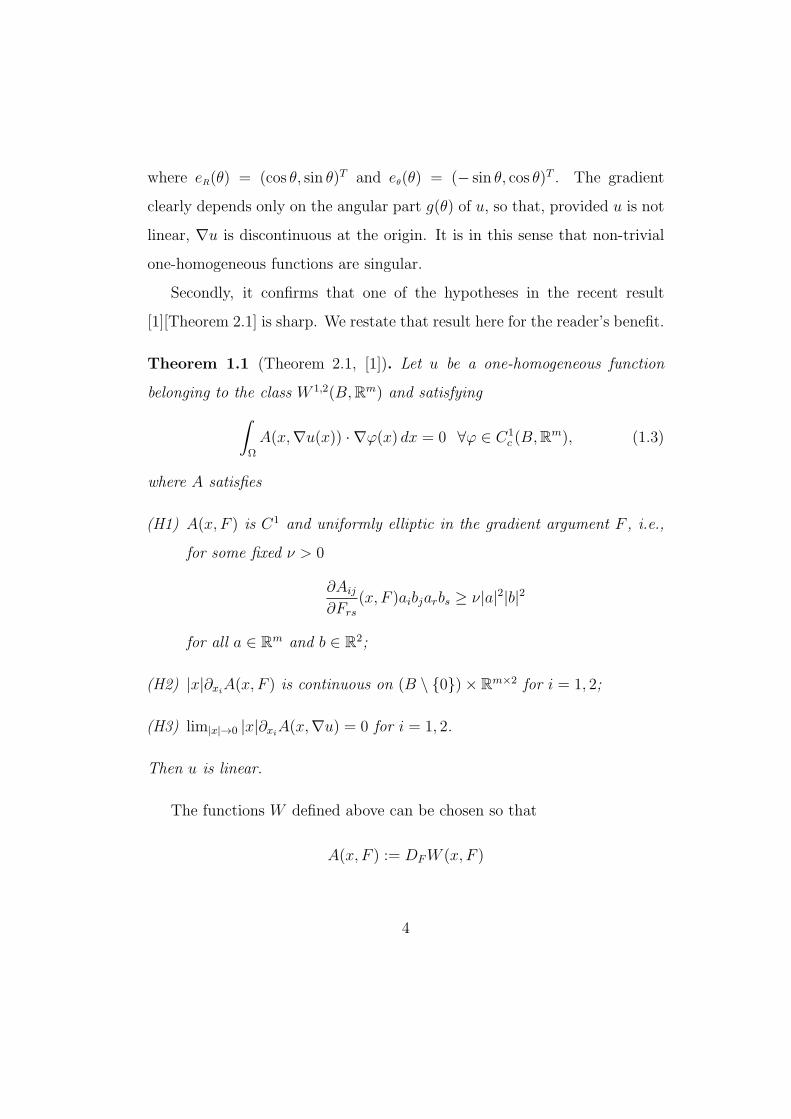
where eR(θ) = (cos θ, sin θ)T and eθ(θ) = (− sin θ, cos θ)T . The gradient

clearly depends only on the angular part g(θ) of u, so that, provided u is not

linear, ∇u is discontinuous at the origin. It is in this sense that non-trivial

one-homogeneous functions are singular.

Secondly, it confirms that one of the hypotheses in the recent result

[1][Theorem 2.1] is sharp. We restate that result here for the reader’s benefit.

Theorem 1.1 (Theorem 2.1, [1]). Let u be a one-homogeneous function

belonging to the class W 1,2(B,Rm) and satisfying

∫

Ω

A(x,∇u(x)) · ∇ϕ(x) dx = 0 ∀ϕ ∈ C1c (B,R

m), (1.3)

where A satisfies

(H1) A(x, F ) is C1 and uniformly elliptic in the gradient argument F , i.e.,

for some fixed ν > 0

∂Aij

∂Frs

(x, F )aibjarbs ≥ ν|a|2|b|2

for all a ∈ Rm and b ∈ R

2;

(H2) |x|∂xiA(x, F ) is continuous on (B \ 0)× R

m×2 for i = 1, 2;

(H3) lim|x|→0 |x|∂xiA(x,∇u) = 0 for i = 1, 2.

Then u is linear.

The functions W defined above can be chosen so that

A(x, F ) := DFW (x, F )

4

solves (1.3) with u a suitable non-trivial one-homogeneous function, and such

that it obeys conditions (H1) and (H2) while violating (H3). We infer from

this that condition (H3) is necessary. See Lemma 3.2 for details.

It is natural to ask whether there are circumstances under which the one-

homogeneous solutions, u, say, that we construct are unique. By studying

the stationarity condition (1.1) in the planar case, we give a necessary and,

under some additional assumptions, sufficient condition for uniqueness. See

Propositions 3.3 and 3.4 for details.

In view of the fact that the u solves an Euler-Lagrange equation, it is

also natural to ask whether these solutions arise as minimizers of appropri-

ate variational problems. It turns out that they do in least two cases: one

corresponding to a problem in which functions u competing in the minimiza-

tion process are constrained to satisfy det∇u = 1 a.e. (see Section 4.1), and

another corresponding to an unconstrained problem (see Section 4.2) which

has some remarkable similarities to a system constructed by Meyers in [10].

The paper is accordingly divided into three parts: Section 2 gives the con-

struction of a general class of one-homogeneous solutions to the PDE problem

(1.1); Section 3 considers among other things the question of uniqueness re-

ferred to above, and Section 4 is devoted to a variational interpretation of

the results of Section 2.

2. One-homogeneous solutions

2.1. Notation

We denote the m×n real matrices by Rm×n, and unless stated otherwise

we sum over repeated indices. Other standard notation includes || · ||k,p;Ω

5

for the norm on the Sobolev space W k,p(Ω), || · ||p;Ω for the norm on Lp(Ω),

and ,∗ to represent weak and weak∗ convergence respectively in both of

these spaces. Here, Ω is a domain in Rn. As usual, we denote by B(a,R) the

ball in Rn centred at a with radius R. When the ball has centre zero and

radius r we write Br, and when the radius is 1 we simply write B for B1.

H1(Ω) represents the Hardy space dual to BMO(Ω), the space of functions of

Bounded Mean Oscillation (see [5, 2]). In keeping with the general literature,

we use H1 and L2 to represent one-dimensional Hausdorff measure and two-

dimensional Lebesgue measure respectively. It will be clear from the context

whether H1 refers to Hardy space or 1− dimensional Hausdorff measure.

Unless stated otherwise, the letters a.e. refer to L2−almost everywhere.

The tensor product of two vectors a ∈ Rm and b ∈ R

n is written a ⊗ b

and is the m × n matrix whose (i, j) entry is aibj. The inner product of

two matrices F1, F2 ∈ Rm×n is F1 · F2 = tr (F T

1 F2). This obviously holds for

vectors too. Throughout, we use this inner product to define the norm |F |on matrices F via |F |2 = F · F .

In plane polar coordinates (R, θ) the gradient of ϕ : R2 → Rm is

∇ϕ = ϕ,R ⊗eR(θ) + ϕ,τ ⊗eθ(θ), (2.1)

where eR(θ) = (cos θ, sin θ)T , eθ(θ) = (− sin θ, cos θ)T and

ϕ,τ =1

Rϕ,θ

provided R 6= 0. We write ϕ,R = for the partial derivative of ϕ with respect

to R, and similarly for ϕ,θ. In this notation the formula

det∇ϕ = Jϕ,R ·ϕ,τ (2.2)

6

holds, where J is the 2 × 2 matrix corresponding to a rotation of π2radians

in the plane, i.e.,

J =

0 1

−1 0

.

Two useful properties of J are that (i) JT = −J , so that in particular

a · Jb = −Ja · b for any two a, b ∈ R2, and (ii) cof A = JTAJ for any 2 × 2

matrix A. For any set Ω we write χΩ for the characteristic (or indicator)

function of Ω. If Ω is an L2−measurable set and g a measurable function

then the integral average of g over Ω is

−∫

Ω

g(x) dx =1

L2(Ω)

∫

Ω

g(x) dx.

A similar definition holds with H1 in place of L2.

2.2. Construction of general one-homogeneous solutions

Let W be as in (1.2). We make some assumptions on the convex function

appearing in (1.2). That is, we suppose that the function f appearing there

is such that:

(h1) f : R+ → R+ is C2 on the open interval (0,∞), with f(0) = f ′(0+) = 0,

and f ′′(t) > 0 for all t > 0;

(h2) f obeys a polynomial growth condition of order p from above, i.e.,

f(|F |) ≤ c(1 + |F |p) ∀ F ∈ Rm×2

for a fixed positive constant c and where p > 1.

Assumptions (h1) and (h2) imply that the function γ : Rm×2 → R defined

by

γ(F ) = f(|F |) (2.3)

7

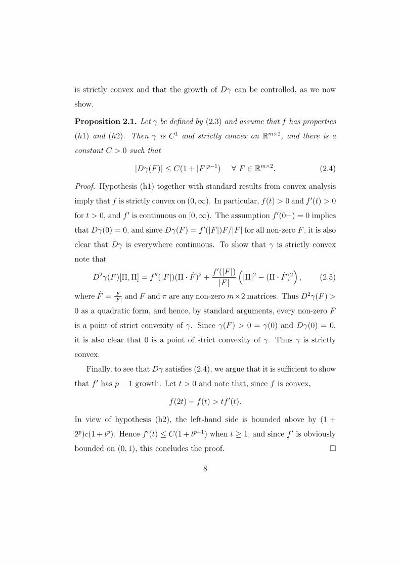
is strictly convex and that the growth of Dγ can be controlled, as we now

show.

Proposition 2.1. Let γ be defined by (2.3) and assume that f has properties

(h1) and (h2). Then γ is C1 and strictly convex on Rm×2, and there is a

constant C > 0 such that

|Dγ(F )| ≤ C(1 + |F |p−1) ∀ F ∈ Rm×2. (2.4)

Proof. Hypothesis (h1) together with standard results from convex analysis

imply that f is strictly convex on (0,∞). In particular, f(t) > 0 and f ′(t) > 0

for t > 0, and f ′ is continuous on [0,∞). The assumption f ′(0+) = 0 implies

that Dγ(0) = 0, and since Dγ(F ) = f ′(|F |)F/|F | for all non-zero F , it is alsoclear that Dγ is everywhere continuous. To show that γ is strictly convex

note that

D2γ(F )[Π,Π] = f ′′(|F |)(Π · F )2 + f ′(|F |)|F |

(|Π|2 − (Π · F )2

), (2.5)

where F = F|F |

and F and π are any non-zerom×2 matrices. Thus D2γ(F ) >

0 as a quadratic form, and hence, by standard arguments, every non-zero F

is a point of strict convexity of γ. Since γ(F ) > 0 = γ(0) and Dγ(0) = 0,

it is also clear that 0 is a point of strict convexity of γ. Thus γ is strictly

convex.

Finally, to see that Dγ satisfies (2.4), we argue that it is sufficient to show

that f ′ has p− 1 growth. Let t > 0 and note that, since f is convex,

f(2t)− f(t) > tf ′(t).

In view of hypothesis (h2), the left-hand side is bounded above by (1 +

2p)c(1 + tp). Hence f ′(t) ≤ C(1 + tp−1) when t ≥ 1, and since f ′ is obviously

bounded on (0, 1), this concludes the proof.

8

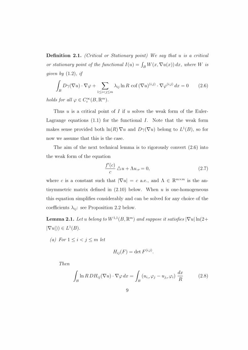
Definition 2.1. (Critical or Stationary point) We say that u is a critical

or stationary point of the functional I(u) =∫BW (x,∇u(x)) dx, where W is

given by (1.2), if∫

B

Dγ(∇u) · ∇ϕ+∑

1≤i<j≤m

λij lnR cof (∇u)(i,j) · ∇ϕ(i,j) dx = 0 (2.6)

holds for all ϕ ∈ C∞c (B,Rm).

Thus u is a critical point of I if u solves the weak form of the Euler-

Lagrange equations (1.1) for the functional I. Note that the weak form

makes sense provided both ln(R)∇u and Dγ(∇u) belong to L1(B), so for

now we assume that this is the case.

The aim of the next technical lemma is to rigorously convert (2.6) into

the weak form of the equation

f ′(c)

cu+ Λu,τ = 0, (2.7)

where c is a constant such that |∇u| = c a.e., and Λ ∈ Rm×m is the an-

tisymmetric matrix defined in (2.10) below. When u is one-homogeneous

this equation simplifies considerably and can be solved for any choice of the

coefficients λij: see Proposition 2.2 below.

Lemma 2.1. Let u belong toW 1,1(B,Rm) and suppose it satisfies |∇u| ln(2+|∇u|)) ∈ L1(B).

(a) For 1 ≤ i < j ≤ m let

Hij(F ) = detF (i,j).

Then∫

B

lnRDHij(∇u) · ∇ϕdx =

∫

B

(ui,τϕj − uj,τϕi)dx

R(2.8)

9

for all ϕ ∈ C∞c (B,Rm).

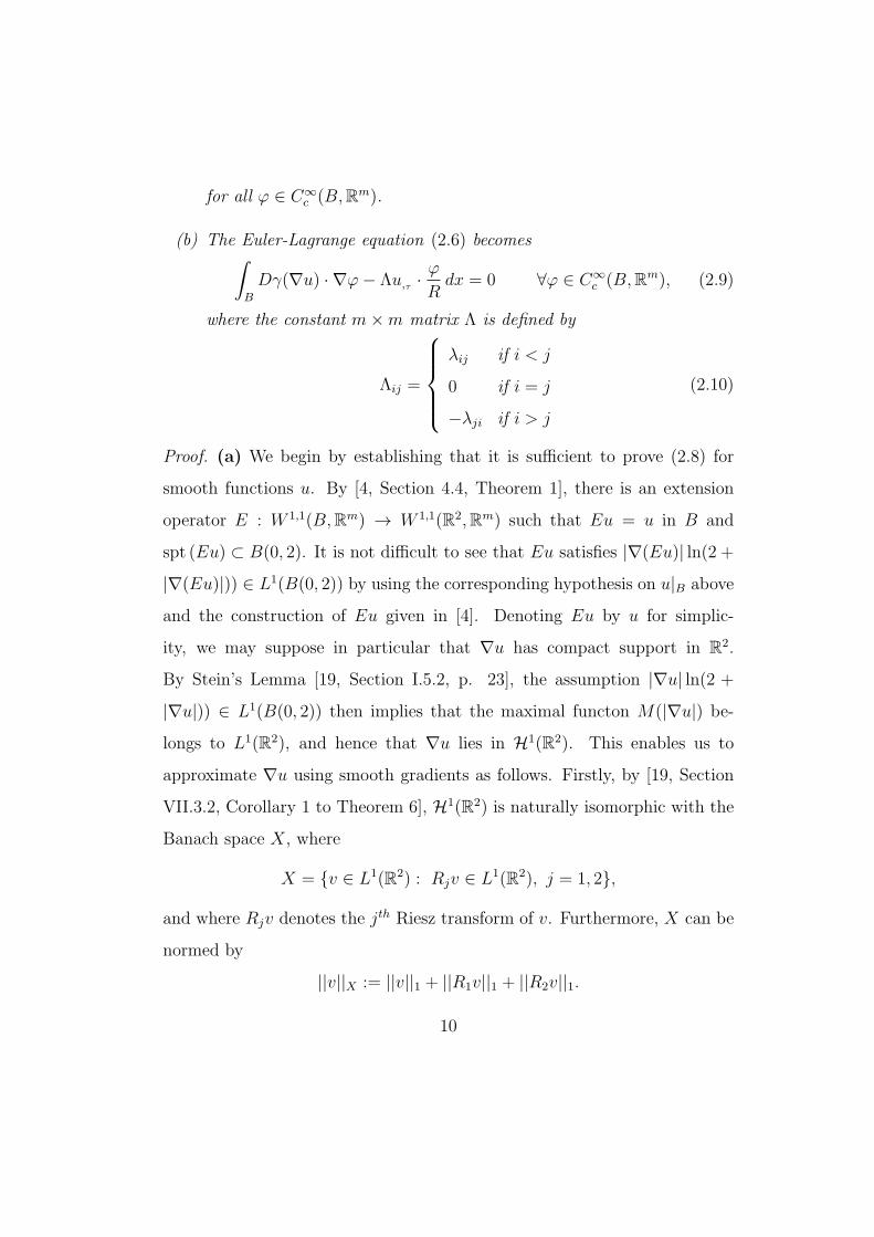
(b) The Euler-Lagrange equation (2.6) becomes∫

B

Dγ(∇u) · ∇ϕ− Λu,τ ·ϕ

Rdx = 0 ∀ϕ ∈ C∞

c (B,Rm), (2.9)

where the constant m×m matrix Λ is defined by

Λij =

λij if i < j

0 if i = j

−λji if i > j

(2.10)

Proof. (a) We begin by establishing that it is sufficient to prove (2.8) for

smooth functions u. By [4, Section 4.4, Theorem 1], there is an extension

operator E : W 1,1(B,Rm) → W 1,1(R2,Rm) such that Eu = u in B and

spt (Eu) ⊂ B(0, 2). It is not difficult to see that Eu satisfies |∇(Eu)| ln(2 +|∇(Eu)|)) ∈ L1(B(0, 2)) by using the corresponding hypothesis on u|B above

and the construction of Eu given in [4]. Denoting Eu by u for simplic-

ity, we may suppose in particular that ∇u has compact support in R2.

By Stein’s Lemma [19, Section I.5.2, p. 23], the assumption |∇u| ln(2 +

|∇u|)) ∈ L1(B(0, 2)) then implies that the maximal functon M(|∇u|) be-

longs to L1(R2), and hence that ∇u lies in H1(R2). This enables us to

approximate ∇u using smooth gradients as follows. Firstly, by [19, Section

VII.3.2, Corollary 1 to Theorem 6], H1(R2) is naturally isomorphic with the

Banach space X, where

X = v ∈ L1(R2) : Rjv ∈ L1(R2), j = 1, 2,

and where Rjv denotes the jth Riesz transform of v. Furthermore, X can be

normed by

||v||X := ||v||1 + ||R1v||1 + ||R2v||1.

10

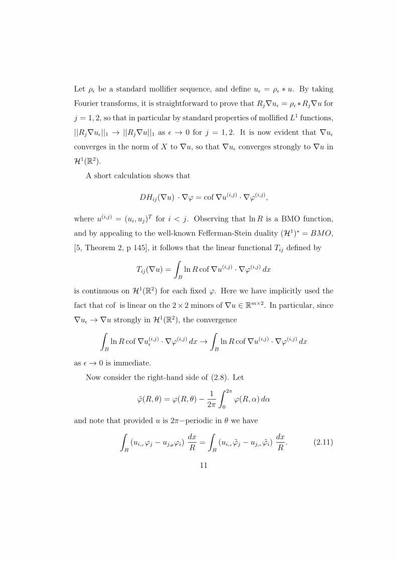
Let ρǫ be a standard mollifier sequence, and define uǫ = ρǫ ∗ u. By taking

Fourier transforms, it is straightforward to prove that Rj∇uǫ = ρǫ∗Rj∇u for

j = 1, 2, so that in particular by standard properties of mollified L1 functions,

||Rj∇uǫ||1 → ||Rj∇u||1 as ǫ → 0 for j = 1, 2. It is now evident that ∇uǫconverges in the norm of X to ∇u, so that ∇uǫ converges strongly to ∇u in

H1(R2).

A short calculation shows that

DHij(∇u) · ∇ϕ = cof∇u(i,j) · ∇ϕ(i,j),

where u(i,j) = (ui, uj)T for i < j. Observing that lnR is a BMO function,

and by appealing to the well-known Fefferman-Stein duality (H1)∗ = BMO,

[5, Theorem 2, p 145], it follows that the linear functional Tij defined by

Tij(∇u) =∫

B

lnR cof∇u(i,j) · ∇ϕ(i,j) dx

is continuous on H1(R2) for each fixed ϕ. Here we have implicitly used the

fact that cof is linear on the 2×2 minors of ∇u ∈ Rm×2. In particular, since

∇uǫ → ∇u strongly in H1(R2), the convergence

∫

B

lnR cof∇u(i,j)ǫ · ∇ϕ(i,j) dx→∫

B

lnR cof∇u(i,j) · ∇ϕ(i,j) dx

as ǫ→ 0 is immediate.

Now consider the right-hand side of (2.8). Let

ϕ(R, θ) = ϕ(R, θ)− 1

2π

∫ 2π

0

ϕ(R,α) dα

and note that provided u is 2π−periodic in θ we have

∫

B

(ui,τϕj − uj,θϕi)dx

R=

∫

B

(ui,τ ϕj − uj,τ ϕi)dx

R. (2.11)

11

Since ϕ is smooth, it follows in particular that ϕRhas a removable singularity

at the origin, and is otherwise bounded. Writing the right-hand side of (2.11)

as ∫

B

ϕ(i,j)

R· J∇u(i,j)eR dx,

it is therefore clear that we can pass to the limit ǫ→ 0 in

∫

B

ϕ(i,j)

R· J∇u(i,j)ǫ eR dx,

and replace ϕ with ϕ. In summary, it is sufficient to prove (2.8) for smooth

functions u.

To that end, in the following we integrate by parts and then use the fact

that cof∇u is divergence free whenever u is a smooth planar map.

∫

B

lnRDHij(∇u) · ∇ϕdx =

∫

B

lnR cof∇u(i,j) · ∇ϕ(i,j) dx

= −∫

B

ϕ(i,j) · cof∇u(i,j) eRRdx

=

∫

B

ϕ(i,j) · Ju(i,j)τ

dx

R

=

∫

B

(ui,τϕj − uj,τϕi)dx

R,

so proving (2.8).

(b) The Euler-Lagrange equation (2.6) may be written

∫

B

Dγ(∇u) · ∇ϕ+∑

1≤i<j≤m

λij lnR DHij(∇u) · ∇ϕdx = 0.

Applying (2.8) it follows that

∫

B

Dγ(∇u) · ∇ϕdx+∑

1≤i<j≤m

∫

B

λij (ui,τϕj − uj,τϕi)dx

R= 0.

12

Fix an index k in 1, . . . ,m and note that the terms involving ϕk in the

second of these integrals are

−∫

B

∑

k<j≤m

λkjuj,τϕkdx

R+

∫

B

∑

1≤i<k

λikui,τϕkdx

R,

which, in terms of the matrix Λ defined in (2.10), equals∫B−Λu,τ · ϕ

Rdx, as

required.

Proposition 2.2. Let the m×m matrix Λ defined by (2.10) in the statement

of Lemma 2.1 be non-zero. Assume that the function f appearing in (3.4)

satisfies hypothesis (h1). Then

(a) there exist one-homogeneous solutions u(R, θ) = Rg(θ) to the Euler-

Lagrange equation (2.9) such that g obeys the equation

|g|2 + |g′|2 = c2 (2.12)

for some constant c, and such that

(i) u is linear if m is an odd integer, or if m is even and Λ has a

non-trivial kernel;

(ii) u is non-linear and the set u(B) is homeomorphic to a two dimen-

sional disk in Rm covered k times, k ∈ N \ 1, provided f is such

that ((k2 − 1)f ′(t)

kt

)2

lies in the (non-zero) spectrum of −Λ2 for some t > 0.

(b) Any one-homogeneous solution u = Rg to (2.9) such that g is of class

C2(S1,Rm) satisfies (2.12) for some constant c. In particular, g satis-

13

fiesf ′(c)

c(g′′ + g) + Λg′ = 0 (2.13)

on [0, 2π].

Proof. (a) Let g(θ) = ξ cos(kθ)+η sin(kθ) for fixed orthogonal vectors ξ, η ∈R

m and an integer k to be determined shortly. With u = Rg(θ), (2.1) implies

that

∇u = g(θ)⊗ eR(θ) + g′(θ)⊗ eθ(θ),

and so (2.12) is equivalent to the statement |∇u| = c. It holds if and only if

either k2 = 1 or |ξ| = |η|. In either case, (2.9) becomes

∫

B

(f ′(c)

c(g′′ + g) + Λg′

)· ϕRdx = 0

for all ϕ ∈ C∞c (B,Rm). Therefore in order to solve (2.9), and hence (2.6), it

is sufficient to ensure that g satisfies (2.13). We consider two cases, the first

of which corresponds to finding a linear solution of (2.9).

Case (a)(i) If k2 = 1 then clearly g′′+g = 0, and (2.13) holds only if Λξ and

Λη both vanish. If m is odd then the skew-symmetry of Λ guarantees the

existence of ξ (and hence of η by taking η = ξ), while if m is even solutions

corresponding to k2 = 1 exist only if ker Λ is non-zero.

Case (a)(ii) When k 6= 1 equation (2.13) holds only if

ρξ + Λη = 0 (2.14)

ρη − Λξ = 0,

where ρ := f ′(c)(1−k2)kc

. Necessarily, Λ2ξ = −ρ2ξ. Note that if this can be

solved for ρ 6= 0 then defining η by the second of the above equations, namely

14

η = 1ρΛξ, yields a solution to the first. Moreover, η so defined automatically

satisfies |η| = |ξ|, which is needed in order that (2.12) holds, and since

ξ · Λξ = 0 (because Λ is skew), it follows that ξ and η are orthogonal.

Therefore it is sufficient to find ξ such that Λξ = −ρ2ξ for some non-zero

ρ. To this end, observe that the matrix −Λ2 is positive semi-definite and

symmetric, and so has a diagonal representation Diag(ρ12, . . . , ρm

2) in terms

of an appropriate basis, with ρj real for 1 ≤ j ≤ m. Therefore there exists

a non-zero eigenvalue for Λ2 provided Λ2 6= 0. But Λ2 = 0 only if all its

diagonal entries vanish, and since each such entry is the Euclidean norm of a

row (equivalently column) of Λ it must be that Λ2 = 0 is possible only when

Λ = 0, contradicting our hypothesis. Finally, we suppose that the integer k

is such that the condition on f stated in (a)(ii) above holds, so that there is

a non-zero eigenvalue ρ02 of −Λ2 such that

(k2 − 1)f ′(t)

kt= ρ0 (2.15)

for some t > 0. Choose ξ so that |ξ| = t(k2 + 1)−1

2 . Recalling that c2 =

(1 + k2)|ξ|2, we see that this choice implies t = c, and hence from (2.15)

(k2 − 1)f ′(c)

kc= ρ0.

From this it follows that equations (2.14) hold with ρ = ρ0 and ξ, η as

described above.

(b) Let P (θ) = |g|2 + |g′|2 and suppose that (2.9) holds. Let

z =f ′(

√P )√P

when P > 0, and set z = 0 when P = 0. It is straightforward to check that

the assumptions on f imply that z vanishes if and only if P vanishes.

15

Integrating by parts in (2.9) we obtain

∫

B

((zg′)′ + zg + Λg′) · ϕdR dθ = 0

for all ϕ ∈ C∞c (B,Rm), and the regularity assumptions on g then imply that

(zg′)′ + zg + Λg′ = 0 (2.16)

at all θ such that P (θ) > 0. Now let N = θ ∈ [0, 2π] : P (θ) > 0. We

shall show in the following that N is either empty, in which case (2.12) holds

trivially, or N = [0, 2π].

First note that since Λ is skew, it follows that g′ ·Λg′ = 0, and hence from

(2.16) that

z(g′′ · g′ + g′ · g) + z′|g′|2 = 0

for θ ∈ N . Furthermore, z(θ) > 0 for θ ∈ N , so that the latter equation

implies in particular that

1

2zP ′ + z′|g′|2 = 0

on N . On using the definition of z given above, we obtain

1

2P ′

(z(√P ) +

z(√P )|g′|2√P

)= 0 (2.17)

on N . Here, z(t) = ddt(f ′(t)/t).

We claim that (2.17) implies that P ′ = 0 on N . Suppose for a contradic-

tion that P ′(θ) 6= 0 for some θ ∈ N . Then, by (2.17),

z(√P ) +

z(√P )|g′|2√P

= 0,

16

which holds only if both terms are non-zero, and in particular when z(√P ) <

0. But then

z(√P ) = |z(

√P )| |g

′|2√P

≤ |z(√P )|

√P

= −f ′′(√P ) +

f ′(√P )√P

,

which, when the definition of z is recalled, gives f ′′(√P ) ≤ 0, contradict-

ing the hypothesis on f . It follows that P ′ = 0 on the set N , and since P

is continuous it must be that if N is non-empty then it covers all of [0, 2π].

Clearly (2.12) then holds, which concludes the proof of part (b) of the propo-

sition.

3. Properties of and conditions for uniqueness of critical points

In this section we restrict attention to the planar case m = 2 and consider

the functionals

G(u) :=

∫

Br

γ(∇u) + λ lnR det∇u dx (3.1)

where Br ⊂ R2. The function γ is defined in (2.3) and f is assumed to satisfy

hypotheses (h1) and (h2). Admissible functions u belong to the class

Ap := u ∈ W 1,p(Br;R2) : u = u on ∂Br, G(u) > −∞, (3.2)

where λ 6= 0 and the exponent p satisfies p > 1. The function u appearing

as a boundary condition in (3.2) will be a one-homogeneous critical point of

the functional G, whose existence is proved in Proposition 3.2 below.

17

That u defined in (3.4) is a critical point of G then implies various facts

about other, suitably regular critical points of the functional G, should they

exist, in the class Ap defined in (3.2). For further details see Propositions

3.3 and 3.4 below. In particular, we give a geometric condition which, when

satisfied, implies that u is the unique critical point of G. The strict mono-

tonicity of Dγ, which can be inferred Proposition (2.1), plays an important

role in the calculations: see Lemma 3.2 for the details.

Proposition 3.1. Let f satisfy hypotheses (h1) and (h2) and suppose that

either f or λ is chosen so that

(k2 − 1)f ′(t)

kt= λ (3.3)

for some t > 0 and some natural number k. Then the k-covering map

u(R, θ) = t(1 + k2)−1

2ReR(kθ) (3.4)

is a stationary point of the functional G defined in (3.1).

Proof. Let u = Rg(θ), where g : S1 → R

2 is C2. Then, by part (b) of

Proposition 2.2, |∇u|2 = c2 for some constant c, and equation (2.13) holds

with

Λ =

0 λ

−λ 0

. (3.5)

According to part (a)(i) of Proposition 2.2, linear solutions exist only if Λ has

a non-trivial kernel, which it plainly does not. Applying (3.3), we suppose

there is an integer k > 1 and t > 0 such that

(k2 − 1)f ′(t)

kt= λ.

18

In these circumstances,

g(θ) = ξ cos kθ + η sin kθ

where −Λ2ξ = λ2ξ and η = 1λΛξ. But −Λ2 = λ21, so that the choice of ξ

|ξ|is

free. We may therefore let ξ = |ξ|e1 and η = |ξ|e2, where

|ξ| = t(1 + k2)−1

2 ,

and hence

g(θ) = t(1 + k2)−1

2 eR(kθ)

for all θ. Hence (3.4).

The resulting one-homogeneous map u is thus proportional to the k-

covering map. Let us write the constant of proportionality as

a = t(1 + k2)−1

2 , (3.6)

so that (3.4) can equivalently be written as

u(R, θ) = aReR(kθ). (3.7)

We briefly return to the discussion of Theorem 1.1, where it was claimed

that if hypothesis (H3) is dropped then the result no longer holds. The result

of Proposition 3.1 above can be used to prove this claim, as follows.

Proposition 3.2. Let γ be defined by (2.3) and assume that f has properties

(h1) and (h2) and that equation (3.3) holds. Suppose in addition that there

is a constant ν > 0 such that f ′′(t) ≥ ν for all t > 0. Then the function

W (x, F ) = γ(F ) + λ lnR detF

19

is such that

A(x, F ) := DFW (x, F )

satisfies hypotheses (H1), (H2) but not (H3) of Theorem 1.1. System (1.3)

is solved by the one-homogeneous function u defined in (3.4).

Proof. The first three assumptions on f ensure that Proposition (3.1) applies,

so that u defined by (3.4) solves (1.3). Next, using the calculation of D2γ

given in (2.5) together with the assumption f ′′ ≥ ν, we find that

D2γ(F )[Π,Π] ≥ ν|Π|2

for all F 6= 0 and all 2× 2 matrices Π. To confirm hypotheses (H1) we must

check that

D2FW (x, F )[a⊗ b, a⊗ b] ≥ ν|a⊗ b|2

independently of x. But

D2FW (x, F )[a⊗ b, a⊗ b] = D2γ(F )[a⊗ b, a⊗ b] + 2λ lnR det(a⊗ b)

≥ ν|a⊗ b|2,

and so (H1) holds. (H2) holds because

R∂xiDFW (x, F ) = λ cof F (3.8)

is continuous everywhere. Hypothesis (H3), however is violated: if it were to

hold we would require

limR→0

R∂xiDFW (x, F ) = 0.

But by (3.8) above this is false whenever F 6= 0.

20

The next result will be used in connection with Lemma 3.3.

Lemma 3.1. Let f satisfy hypotheses (h1) and (h2) and equation (3.3).

Suppose that u ∈ Ap is a critical point of the functional G defined in (3.1)

that is C1 in a semi-open annulus x ∈ Br : r − δ < |x| ≤ r for some

δ > 0. Then

∇u(x) = ∇u(x) x ∈ ∂Br.

Proof. Proposition 3.1 implies that u defined by (3.4) is a critical point of G.

An approximation argument using the regularity assumption on u implies

that ∫

Br

Dγ(∇u) · ∇ϕ+ λ lnR cof∇u · ∇ϕdx = 0

holds in particular when ϕ merely vanishes at ∂Br. Similarly,

∫

Br

Dγ(∇u) · ∇ϕ+ λ lnR cof∇u · ∇ϕdx = 0,

so that by subtracting the two and letting

∆ = Dγ(∇u)−Dγ(∇u)

the equation

∫

Br

∆ · ∇ϕ+ λ lnR cof (∇u−∇u) · ∇ϕdx = 0

follows. Using (2.9) and (3.5), the term involving cof (∇u−∇u) ·∇ϕ can be

rewritten as ∫

Br

λJ(∂,τ (u− u)) · ϕR

dx,

giving ∫

Br

∆ · ∇ϕ+λJ(∂,τ (u− u)) · ϕ

Rdx = 0. (3.9)

21

Define the function η(t, ǫ) by

η(t, ǫ) =

0 if 0 ≤ t ≤ r − ǫ

t−(r−ǫ)ǫ

if r − ǫ ≤ t ≤ r,

let ψ = u− u and take ϕ = ηψ in (3.9). The resulting expression involves in

particular the term

∫

Br\Br−ǫ

∆ · ψ ⊗ eRǫ

dx = −∫

Br\Br−ǫ

∆ ·((u,R (r, θ)− u,R (r, θ))⊗ eR +

l(ǫ)

ǫ

),

where the term ǫ−1l(ǫ) → 0 as ǫ→ 0. Using this, (3.9) reads

∫

Br\Br−ǫ

∆ · (η(u,R − u,R)⊗ eR − (u,R(r, θ)− u,R(r, θ))⊗ eR) dx+

+

∫

Br\Br−ǫ

∆ · l(ǫ)ǫ

dx+

+

∫

Br\Br−ǫ

η∆ · (u,θ − u,θ)⊗eθR

+λJ(∂τ (u− u)) · ϕ

Rdx = 0. (3.10)

Since1

ǫ

∫

Br\Br−ǫ

η(x) dx→ r

2as ǫ→ 0,

it is clear from the assumed regularity of u that

1

ǫ

∫

Br\Br−ǫ

η∆ · (u,R − u,R)⊗ eR dx→ 1

2

∫

∂Br

∆ · (u,R (r, θ)− u,R (r, θ))⊗ eR ds.

Similarly,

1

ǫ

∫

Br\Br−ǫ

η∆·(u,R (r, θ)−u,R (r, θ))⊗eR dx→∫

∂Br

∆·(u,R (r, θ)−u,R (r, θ))⊗eR ds.

Dividing (3.10) by ǫ and letting ǫ→ 0, it follows that

∫

∂Br

∆ · (u,R (r, θ)− u,R (r, θ))⊗ eR ds = 0. (3.11)

22

Now, in view of u = u on ∂Br, ∇u − ∇u = (u,R (r, θ) − u,R (r, θ)) ⊗ eR on

∂Br, so that (3.11) becomes

∫

∂Br

(Dγ(∇u)−Dγ(∇u)) · (∇u−∇u) ds = 0. (3.12)

By Proposition 2.1, γ is C1 and strictly convex, and hence, by standard

results from convex analysis, Dγ is strictly monotone. It follows that (3.12)

holds only if ∇u = ∇u on ∂Br, concluding the proof.

A second and more immediate consequence of the strict monotonicity of

Dγ is contained in the next result. Note that it applies to any two critical

points of G.

Proposition 3.3. Let G be defined by (3.1) and let u1 and u2 be critical

points of G in Ap. Then

∫

Br

lnR det(∇u1 −∇u2) dx ≤ 0

with equality if and only if u1 = u2 a.e. in Br.

Proof. By definition, the critical points u1 and u2 satisfy

∫

Br

Dγ(∇uj) · ∇ϕ+ λ lnR cof∇uj · ∇ϕdx = 0,

j = 1, 2, for all smooth test functions ϕ with compact support in the ball Br.

Subtracting the two equations and letting w = u1 − u2 yields

∫

Br

(Dγ(∇u1)−Dγ(∇u2)) · ∇ϕ+ λ lnR cof∇w · ∇ϕdx = 0

for all such ϕ. By an approximation argument we may take ϕ = w in the

above. To be specific, the first term can be approximated by first applying

23

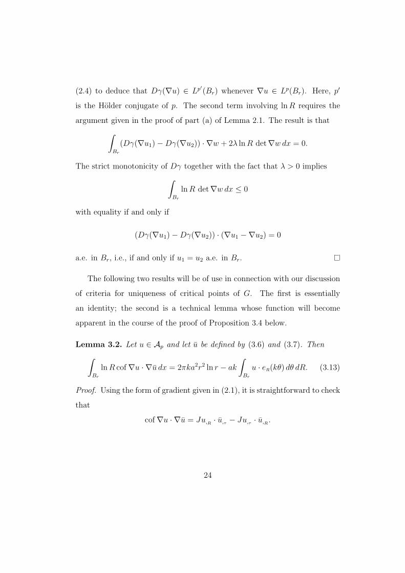
(2.4) to deduce that Dγ(∇u) ∈ Lp′(Br) whenever ∇u ∈ Lp(Br). Here, p′

is the Holder conjugate of p. The second term involving lnR requires the

argument given in the proof of part (a) of Lemma 2.1. The result is that

∫

Br

(Dγ(∇u1)−Dγ(∇u2)) · ∇w + 2λ lnR det∇w dx = 0.

The strict monotonicity of Dγ together with the fact that λ > 0 implies

∫

Br

lnR det∇w dx ≤ 0

with equality if and only if

(Dγ(∇u1)−Dγ(∇u2)) · (∇u1 −∇u2) = 0

a.e. in Br, i.e., if and only if u1 = u2 a.e. in Br.

The following two results will be of use in connection with our discussion

of criteria for uniqueness of critical points of G. The first is essentially

an identity; the second is a technical lemma whose function will become

apparent in the course of the proof of Proposition 3.4 below.

Lemma 3.2. Let u ∈ Ap and let u be defined by (3.6) and (3.7). Then

∫

Br

lnR cof∇u · ∇u dx = 2πka2r2 ln r − ak

∫

Br

u · eR(kθ) dθ dR. (3.13)

Proof. Using the form of gradient given in (2.1), it is straightforward to check

that

cof∇u · ∇u = Ju,R · u,τ − Ju,τ · u,R .

24

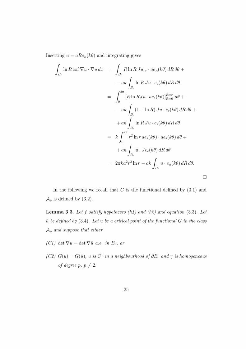
Inserting u = aReR(kθ) and integrating gives

∫

Br

lnR cof∇u · ∇u dx =

∫

Br

R lnRJu,R · aeR(kθ) dR dθ +

− ak

∫

Br

lnRJu · eθ(kθ) dR dθ

=

∫ 2π

0

[R lnRJu · aeθ(kθ)]R=rR=0 dθ +

− ak

∫

Br

(1 + lnR) Ju · eθ(kθ) dR dθ +

+ ak

∫

Br

lnRJu · eθ(kθ) dR dθ

= k

∫ 2π

0

r2 ln r aeθ(kθ) · aeθ(kθ) dθ +

+ ak

∫

Br

u · Jeθ(kθ) dR dθ

= 2πka2r2 ln r − ak

∫

Br

u · eR(kθ) dR dθ.

In the following we recall that G is the functional defined by (3.1) and

Ap is defined by (3.2).

Lemma 3.3. Let f satisfy hypotheses (h1) and (h2) and equation (3.3). Let

u be defined by (3.4). Let u be a critical point of the functional G in the class

Ap and suppose that either

(C1) det∇u = det∇u a.e. in Br, or

(C2) G(u) = G(u), u is C1 in a neighbourhood of ∂Br and γ is homogeneous

of degree p, p 6= 2.

25

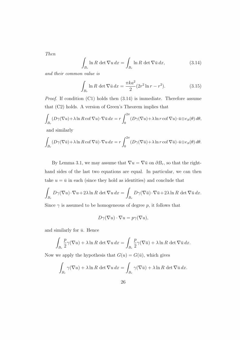
Then ∫

Br

lnR det∇u dx =

∫

Br

lnR det∇u dx, (3.14)

and their common value is∫

Br

lnR det∇u dx =πka2

2(2r2 ln r − r2). (3.15)

Proof. If condition (C1) holds then (3.14) is immediate. Therefore assume

that (C2) holds. A version of Green’s Theorem implies that∫

Br

(Dγ(∇u)+λ lnR cof∇u)·∇u dx = r

∫ 2π

0(Dγ(∇u)+λ ln r cof∇u)·u⊗eR(θ) dθ,

and similarly∫

Br

(Dγ(∇u)+λ lnR cof∇u)·∇u dx = r

∫ 2π

0(Dγ(∇u)+λ ln r cof∇u)·u⊗eR(θ) dθ.

By Lemma 3.1, we may assume that ∇u = ∇u on ∂Br, so that the right-

hand sides of the last two equations are equal. In particular, we can then

take u = u in each (since they hold as identities) and conclude that∫

Br

Dγ(∇u) ·∇u+2λ lnR det∇u dx =

∫

Br

Dγ(∇u) ·∇u+2λ lnR det∇u dx.

Since γ is assumed to be homogeneous of degree p, it follows that

Dγ(∇u) · ∇u = pγ(∇u),

and similarly for u. Hence∫

Br

p

2γ(∇u) + λ lnR det∇u dx =

∫

Br

p

2γ(∇u) + λ lnR det∇u dx.

Now we apply the hypothesis that G(u) = G(u), which gives∫

Br

γ(∇u) + λ lnR det∇u dx =

∫

Br

γ(∇u) + λ lnR det∇u dx.

26

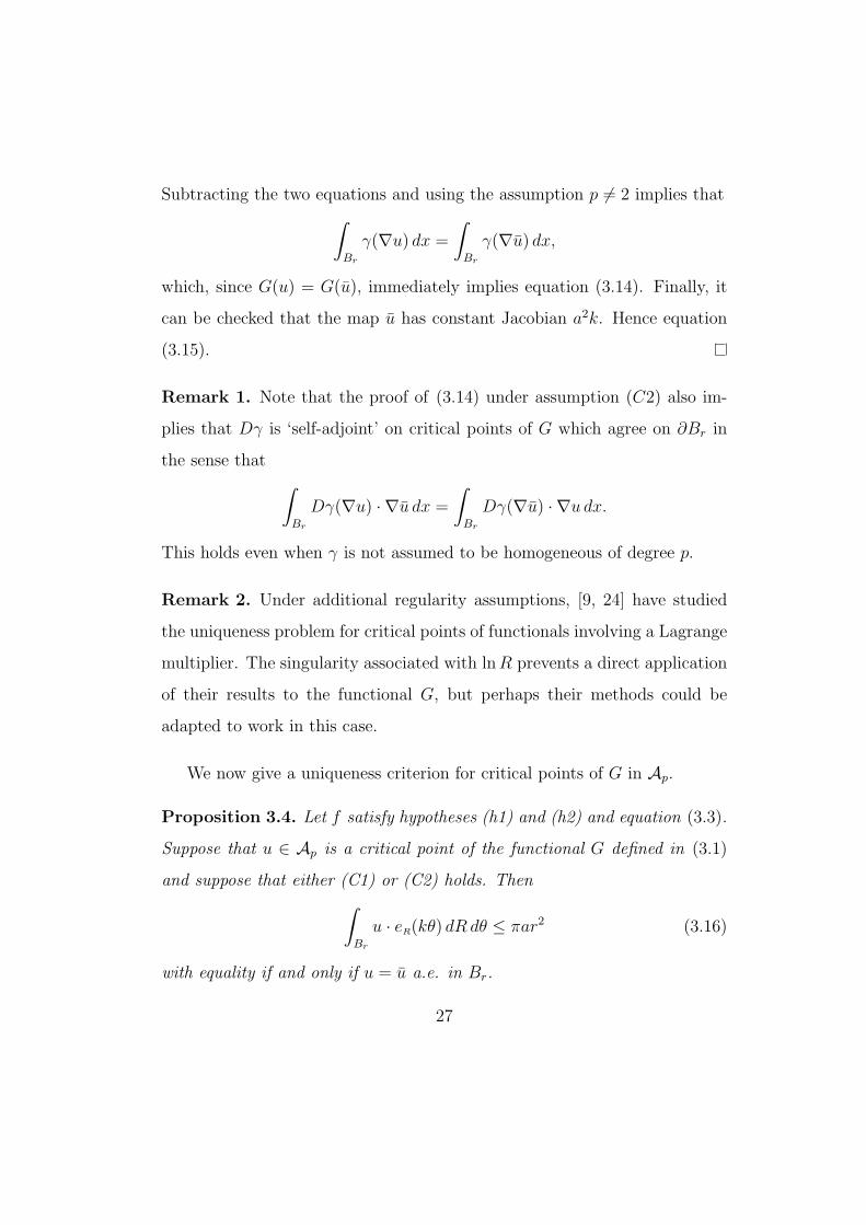
Subtracting the two equations and using the assumption p 6= 2 implies that

∫

Br

γ(∇u) dx =

∫

Br

γ(∇u) dx,

which, since G(u) = G(u), immediately implies equation (3.14). Finally, it

can be checked that the map u has constant Jacobian a2k. Hence equation

(3.15).

Remark 1. Note that the proof of (3.14) under assumption (C2) also im-

plies that Dγ is ‘self-adjoint’ on critical points of G which agree on ∂Br in

the sense that

∫

Br

Dγ(∇u) · ∇u dx =

∫

Br

Dγ(∇u) · ∇u dx.

This holds even when γ is not assumed to be homogeneous of degree p.

Remark 2. Under additional regularity assumptions, [9, 24] have studied

the uniqueness problem for critical points of functionals involving a Lagrange

multiplier. The singularity associated with lnR prevents a direct application

of their results to the functional G, but perhaps their methods could be

adapted to work in this case.

We now give a uniqueness criterion for critical points of G in Ap.

Proposition 3.4. Let f satisfy hypotheses (h1) and (h2) and equation (3.3).

Suppose that u ∈ Ap is a critical point of the functional G defined in (3.1)

and suppose that either (C1) or (C2) holds. Then

∫

Br

u · eR(kθ) dR dθ ≤ πar2 (3.16)

with equality if and only if u = u a.e. in Br.

27

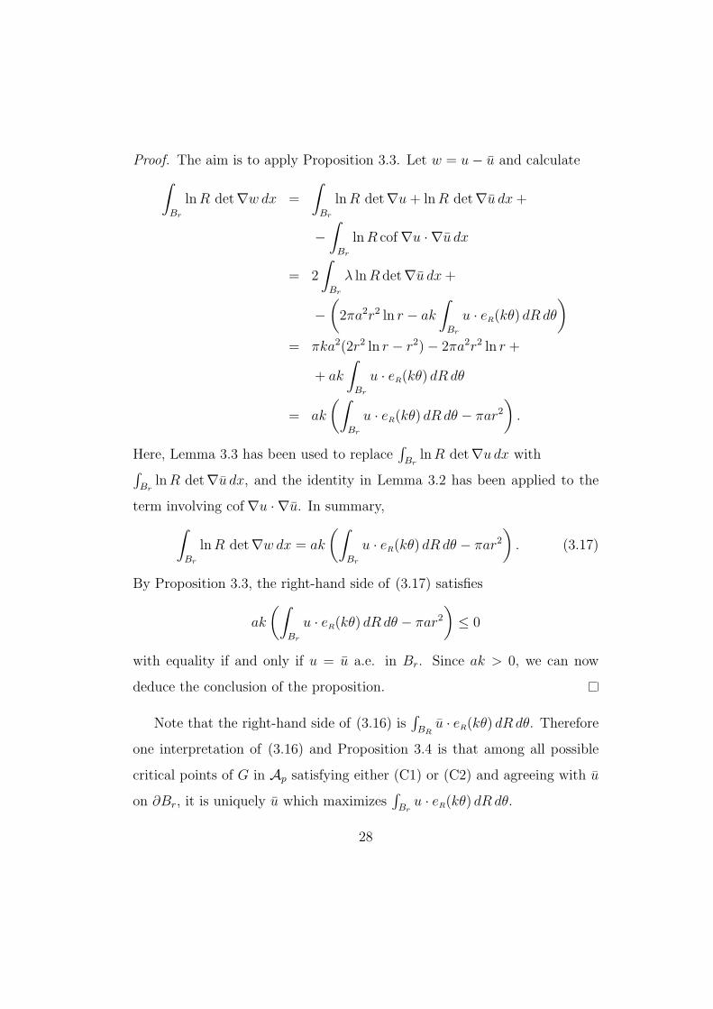
Proof. The aim is to apply Proposition 3.3. Let w = u− u and calculate

∫

Br

lnR det∇w dx =

∫

Br

lnR det∇u+ lnR det∇u dx+

−∫

Br

lnR cof∇u · ∇u dx

= 2

∫

Br

λ lnR det∇u dx+

−(2πa2r2 ln r − ak

∫

Br

u · eR(kθ) dR dθ)

= πka2(2r2 ln r − r2)− 2πa2r2 ln r +

+ ak

∫

Br

u · eR(kθ) dR dθ

= ak

(∫

Br

u · eR(kθ) dR dθ − πar2).

Here, Lemma 3.3 has been used to replace∫Br

lnR det∇u dx with∫Br

lnR det∇u dx, and the identity in Lemma 3.2 has been applied to the

term involving cof∇u · ∇u. In summary,

∫

Br

lnR det∇w dx = ak

(∫

Br

u · eR(kθ) dR dθ − πar2). (3.17)

By Proposition 3.3, the right-hand side of (3.17) satisfies

ak

(∫

Br

u · eR(kθ) dR dθ − πar2)

≤ 0

with equality if and only if u = u a.e. in Br. Since ak > 0, we can now

deduce the conclusion of the proposition.

Note that the right-hand side of (3.16) is∫BRu · eR(kθ) dR dθ. Therefore

one interpretation of (3.16) and Proposition 3.4 is that among all possible

critical points of G in Ap satisfying either (C1) or (C2) and agreeing with u

on ∂Br, it is uniquely u which maximizes∫Bru · eR(kθ) dR dθ.

28

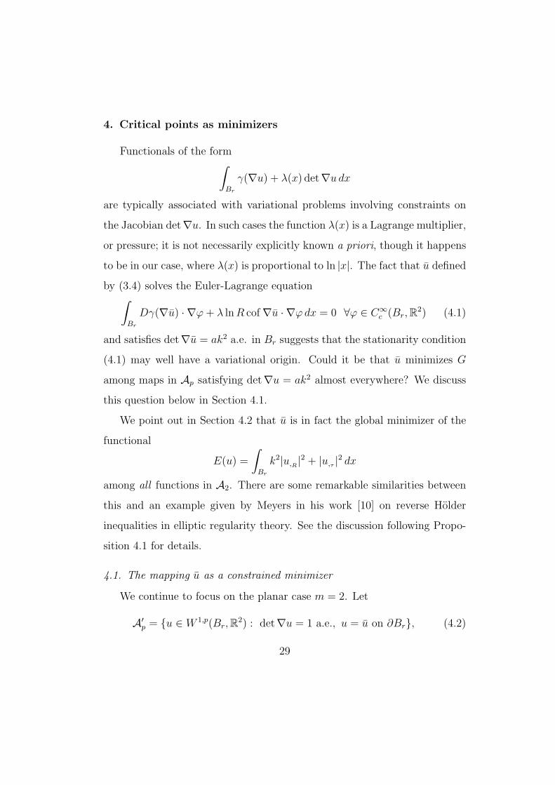
4. Critical points as minimizers

Functionals of the form∫

Br

γ(∇u) + λ(x) det∇u dx

are typically associated with variational problems involving constraints on

the Jacobian det∇u. In such cases the function λ(x) is a Lagrange multiplier,

or pressure; it is not necessarily explicitly known a priori, though it happens

to be in our case, where λ(x) is proportional to ln |x|. The fact that u defined

by (3.4) solves the Euler-Lagrange equation∫

Br

Dγ(∇u) · ∇ϕ+ λ lnR cof∇u · ∇ϕdx = 0 ∀ϕ ∈ C∞c (Br,R

2) (4.1)

and satisfies det∇u = ak2 a.e. in Br suggests that the stationarity condition

(4.1) may well have a variational origin. Could it be that u minimizes G

among maps in Ap satisfying det∇u = ak2 almost everywhere? We discuss

this question below in Section 4.1.

We point out in Section 4.2 that u is in fact the global minimizer of the

functional

E(u) =

∫

Br

k2|u,R |2 + |u,τ |2 dx

among all functions in A2. There are some remarkable similarities between

this and an example given by Meyers in his work [10] on reverse Holder

inequalities in elliptic regularity theory. See the discussion following Propo-

sition 4.1 for details.

4.1. The mapping u as a constrained minimizer

We continue to focus on the planar case m = 2. Let

A′p = u ∈ W 1,p(Br,R

2) : det∇u = 1 a.e., u = u on ∂Br, (4.2)

29

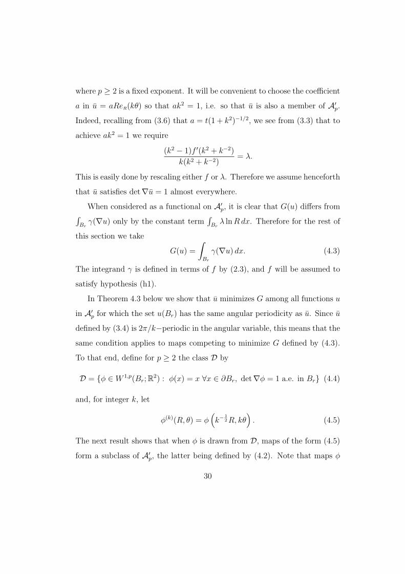
where p ≥ 2 is a fixed exponent. It will be convenient to choose the coefficient

a in u = aReR(kθ) so that ak2 = 1, i.e. so that u is also a member of A′p.

Indeed, recalling from (3.6) that a = t(1 + k2)−1/2, we see from (3.3) that to

achieve ak2 = 1 we require

(k2 − 1)f ′(k2 + k−2)

k(k2 + k−2)= λ.

This is easily done by rescaling either f or λ. Therefore we assume henceforth

that u satisfies det∇u = 1 almost everywhere.

When considered as a functional on A′p, it is clear that G(u) differs from

∫Brγ(∇u) only by the constant term

∫Brλ lnRdx. Therefore for the rest of

this section we take

G(u) =

∫

Br

γ(∇u) dx. (4.3)

The integrand γ is defined in terms of f by (2.3), and f will be assumed to

satisfy hypothesis (h1).

In Theorem 4.3 below we show that u minimizes G among all functions u

in A′p for which the set u(Br) has the same angular periodicity as u. Since u

defined by (3.4) is 2π/k−periodic in the angular variable, this means that the

same condition applies to maps competing to minimize G defined by (4.3).

To that end, define for p ≥ 2 the class D by

D = φ ∈ W 1,p(Br;R2) : φ(x) = x ∀x ∈ ∂Br, det∇φ = 1 a.e. in Br (4.4)

and, for integer k, let

φ(k)(R, θ) = φ(k−

1

2R, kθ). (4.5)

The next result shows that when φ is drawn from D, maps of the form (4.5)

form a subclass of A′p, the latter being defined by (4.2). Note that maps φ

30

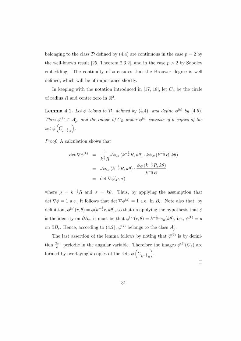
belonging to the class D defined by (4.4) are continuous in the case p = 2 by

the well-known result [25, Theorem 2.3.2], and in the case p > 2 by Sobolev

embedding. The continuity of φ ensures that the Brouwer degree is well

defined, which will be of importance shortly.

In keeping with the notation introduced in [17, 18], let CR be the circle

of radius R and centre zero in R2.

Lemma 4.1. Let φ belong to D, defined by (4.4), and define φ(k) by (4.5).

Then φ(k) ∈ A′p, and the image of CR under φ(k) consists of k copies of the

set φ(C

k−12 R

).

Proof. A calculation shows that

det∇φ(k) =1

k1

2RJφ,R (k

− 1

2R, kθ) · kφ,θ (k−1

2R, kθ)

= Jφ,R (k− 1

2R, kθ) · φ,θ (k− 1

2R, kθ)

k−1

2R= det∇φ(ρ, σ)

where ρ = k−1

2R and σ = kθ. Thus, by applying the assumption that

det∇φ = 1 a.e., it follows that det∇φ(k) = 1 a.e. in Br. Note also that, by

definition, φ(k)(r, θ) = φ(k−1

2 r, kθ), so that on applying the hypothesis that φ

is the identity on ∂Br, it must be that φ(k)(r, θ) = k−1

2 reR(kθ), i.e., φ(k) = u

on ∂Br. Hence, according to (4.2), φ(k) belongs to the class A′p.

The last assertion of the lemma follows by noting that φ(k) is by defini-

tion 2πk−periodic in the angular variable. Therefore the images φ(k)(CR) are

formed by overlaying k copies of the sets φ(C

k−12 R

).

31

Let us suppose that the k appearing in equation (3.4) defining u is fixed.

Define

A′′p = u ∈ W 1,p(Br,R

2) : u = φ(k), φ ∈ D, (4.6)

where p ≥ 2. Note that, by Lemma 4.1, A′′p ⊂ A′

p, and, by inspection, u

belongs to A′′p.

We show in the next two results that u is the global minimizer of G among

maps in the class A′′p. The technical methods we use are an adaptation of

those presented in Sivaloganathan and Spector [17, 18]; we include details of

proofs only to keep the paper self-contained and to avoid confusion with the

scalings involved. In practice, if the reader is already familiar with [17] then

he or she should be able to deduce Theorem 4.3 from Lemma 4.1 and [17,

Section 5].

The notation φtop(Bρ) will be used to denote the topological image of Bρ

under φ: it is defined in terms of the Brouwer degree by

φtop(Bρ) = y ∈ R2 \ φ(Cρ) : d(φ,Bρ, y) 6= 0.

See e.g. [6] for details of the Brouwer degree.

Lemma 4.2. Let u = φ(k) ∈ A′′p. Then for a.e. R ∈ (0, r),

∫

CR

∣∣φ(k),τ∣∣ dH1 ≥ 2πk

1

2R.

Proof. By a change of variables, we see that for all R ∈ (0, r)

∫

CR

∣∣φ(k),τ∣∣ dH1 = k

∫

Ck−

12 R

|φ,τ | dH1. (4.7)

32

Let ρ = k−1

2R. Since φ ∈ W 1,p(Br), it is known that φ|Cρ∈ W 1,p(Cρ) for a.e.

ρ ∈ (0, r). (See [6, Theorem 5.16], for example.) Thus by [20, Theorem 1],

∫

Ck−

12 R

|φ,τ | dH1 ≥ H1(φ(Cρ)) (4.8)

for a.e. ρ ∈ (0, k−1

2 r). Now, by assertion (a) of [12, Lemma 3.5, Step 3],

φ(Cρ) and ∂∗(φtop(Bρ)) are H1−measurable and differ only by a set of H1−

measure zero, with H1(φ(Cρ)) < ∞. Thus a version of the isoperimetric

inequality [26, Theorem 5.4.3] applies to the set φtop(Bρ), giving

H1(∂∗(φtop(Bρ))) ≥ 2π1

2

(L2(φtop(Bρ))

) 1

2 , (4.9)

and hence

H1(φ(Cρ)) ≥ 2π1

2

(L2(φtop(Bρ))

) 1

2 . (4.10)

The proof can be concluded by showing that L2(φtop(Bρ)) = L2(Bρ). To see

this we first claim that d(φ,Bρ, y) = 1 for a.e. y in φ(Bρ), which can be seen

as a consequence of the set

V := y ∈ R2 \ φ(Cρ) : d(φ,Bρ, y) 6= 1 ∩ φ(Bρ).

having L2−measure zero. Let y ∈ V . By the excision and domain decompo-

sition properties of the degree,

d(φ,Br, y) = d(φ,Br \Bρ, y) + d(φ,Bρ, y),

and since φ agrees with the identity map on ∂Br, the left-hand side is 1.

Hence

d(φ,Br \Bρ, y) = 1− d(φ,Bρ, y),

33

which, on using the definition of V , must be non-zero. Thus y has at least

two preimages in Br: at least one in Bρ and at least one in Br \ Bρ. By

[20, Lemma 5.1], the set of such y is L2−null. It follows that L2(V ) = 0, as

claimed, and hence that

(a) d(φ,Bρ, y) = 1 for L2− a.e. y ∈ φ(Bρ) \ φ(Cρ), and

(b) φ(Bρ) and φtop(Bρ) differ by an L2− null set.

To see part (b), note the inclusions φtop(Bρ) ⊂ φ(Bρ) and φ(Bρ)\φtop(Bρ) ⊂V , and then apply L2(V ) = 0.

Finally, we note that the hypotheses of [6, Theorem 5.25] are satisfied, so

that the change of variables formula∫

Bρ

det∇φ dx =

∫

R2

d(φ,Bρ, y) dy.

holds. By hypothesis, det∇φ = 1 a.e., so the left-hand side is L2(Bρ). By (a),

the integral on the right is L2(φ(Bρ)), which by (b) is equal to L2(φtop(Bρ)).

Inserting this information into (4.10), using (4.8), and changing variables

from ρ to R yields the inequality appearing in the statement of the lemma.

We now apply Lemma 4.2 to the functional G defined in (4.3), following

the method of [17, Remark 3.10]

Theorem 4.3. Let u ∈ A′′p, defined by (4.6), let G be the functional defined

by (4.3), and suppose u is given by (3.4). Then G(u) ≥ G(u).

Proof. Let u = φ(k) for some φ ∈ D. Note that since det∇φ(k) = 1 a.e. in

Br, it follows from (2.2) and the Cauchy-Schwarz inequality that

|φ(k),R | ≥1

|φ(k),τ |(4.11)

34

a.e. in Br. Following [17], we first show

∫

Br

|∇u| dx ≥∫

Br

|∇u| dx.

To that end, let

h(s) = (s2 + s−2)1

2

for all s > 0. Note that h is convex on (0,∞) and strictly increasing on

[1,∞). By the coarea formula ([4, Theorem 1, Section 3.4.2]), (4.11), and

Jensen’s inequality,

∫

Br

|∇u| dx =

∫ r

0

∫

CR

(|φ(k),R |2 + |φ(k),τ |2

) 1

2 dH1 dR

≥∫ r

0

∫

CR

(|φ(k),τ |−2 + |φ(k),τ |2

) 1

2 dH1 dR

=

∫ r

0

∫

CR

h(|φ(k),τ |

)dH1 dR

≥∫ r

0

2πRh

(−∫

CR

|φ(k),τ | dH1

)dR. (4.12)

By Lemma 4.2,

−∫

CR

|φ(k),τ | dH1 ≥ k1

2

for a.e. R ∈ (0, r). Since k is a positive integer, it follows that

h

(−∫

CR

|φ(k),τ | dH1

)≥ h(k

1

2 ).

Inserting this into (4.12) and using the fact that u = k−1

2ReR(kθ) satisfies

|∇u| = h(k1

2 ),

we conclude that ∫

Br

|∇u| dx ≥∫

Br

|∇u| dx. (4.13)

35

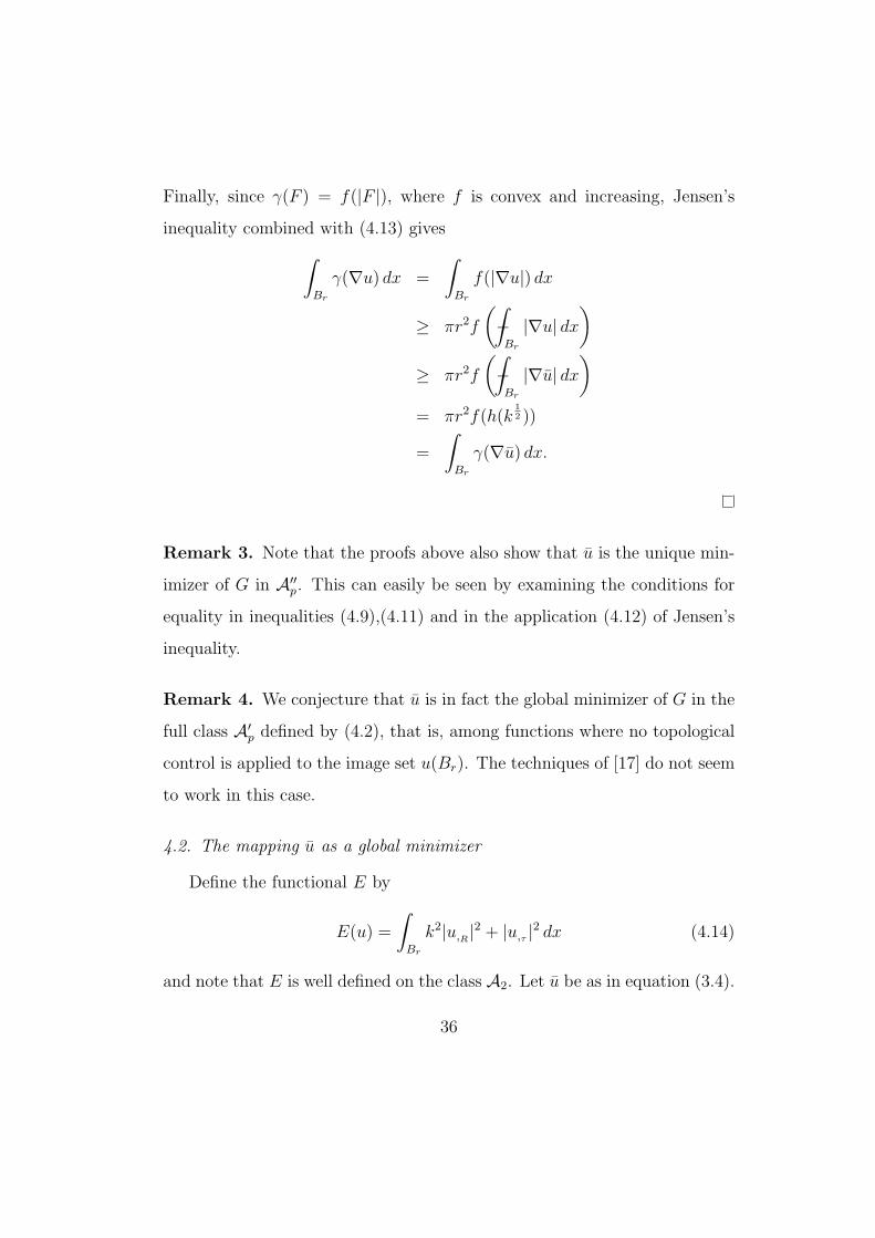
Finally, since γ(F ) = f(|F |), where f is convex and increasing, Jensen’s

inequality combined with (4.13) gives

∫

Br

γ(∇u) dx =

∫

Br

f(|∇u|) dx

≥ πr2f

(−∫

Br

|∇u| dx)

≥ πr2f

(−∫

Br

|∇u| dx)

= πr2f(h(k1

2 ))

=

∫

Br

γ(∇u) dx.

Remark 3. Note that the proofs above also show that u is the unique min-

imizer of G in A′′p. This can easily be seen by examining the conditions for

equality in inequalities (4.9),(4.11) and in the application (4.12) of Jensen’s

inequality.

Remark 4. We conjecture that u is in fact the global minimizer of G in the

full class A′p defined by (4.2), that is, among functions where no topological

control is applied to the image set u(Br). The techniques of [17] do not seem

to work in this case.

4.2. The mapping u as a global minimizer

Define the functional E by

E(u) =

∫

Br

k2|u,R |2 + |u,τ |2 dx (4.14)

and note that E is well defined on the class A2. Let u be as in equation (3.4).

36

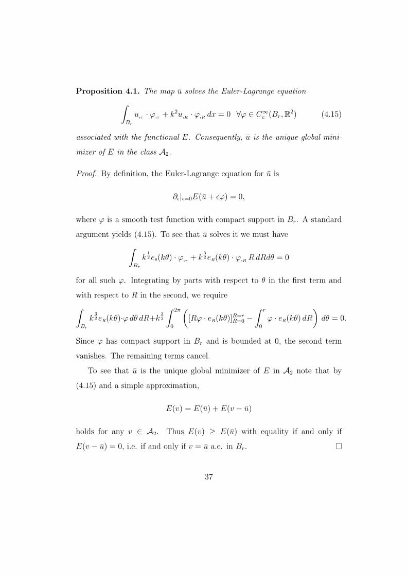
Proposition 4.1. The map u solves the Euler-Lagrange equation

∫

Br

u,τ · ϕ,τ + k2u,R · ϕ,R dx = 0 ∀ϕ ∈ C∞c (Br,R

2) (4.15)

associated with the functional E. Consequently, u is the unique global mini-

mizer of E in the class A2.

Proof. By definition, the Euler-Lagrange equation for u is

∂ǫ|ǫ=0E(u+ ǫϕ) = 0,

where ϕ is a smooth test function with compact support in Br. A standard

argument yields (4.15). To see that u solves it we must have

∫

Br

k1

2 eθ(kθ) · ϕ,τ + k3

2 eR(kθ) · ϕ,R RdRdθ = 0

for all such ϕ. Integrating by parts with respect to θ in the first term and

with respect to R in the second, we require

∫

Br

k3

2 eR(kθ)·ϕdθ dR+k3

2

∫ 2π

0

([Rϕ · eR(kθ)]R=r

R=0 −∫ r

0

ϕ · eR(kθ) dR)dθ = 0.

Since ϕ has compact support in Br and is bounded at 0, the second term

vanishes. The remaining terms cancel.

To see that u is the unique global minimizer of E in A2 note that by

(4.15) and a simple approximation,

E(v) = E(u) + E(v − u)

holds for any v ∈ A2. Thus E(v) ≥ E(u) with equality if and only if

E(v − u) = 0, i.e. if and only if v = u a.e. in Br.

37

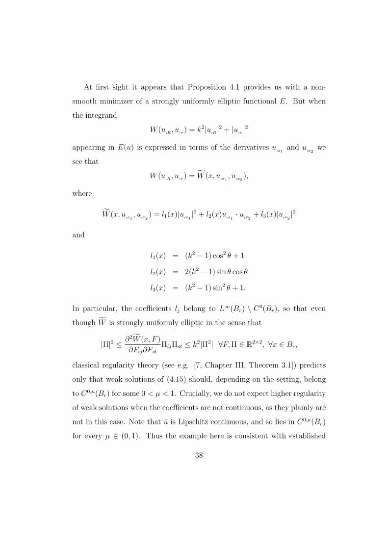
At first sight it appears that Proposition 4.1 provides us with a non-

smooth minimizer of a strongly uniformly elliptic functional E. But when

the integrand

W (u,R , u,τ ) = k2|u,R |2 + |u,τ |2

appearing in E(u) is expressed in terms of the derivatives u,x1 and u,x2 we

see that

W (u,R , u,τ ) = W (x, u,x1 , u,x2 ),

where

W (x, u,x1 , u,x2 ) = l1(x)|u,x1 |2 + l2(x)u,x1 · u,x2 + l3(x)|u,x2 |

2

and

l1(x) = (k2 − 1) cos2 θ + 1

l2(x) = 2(k2 − 1) sin θ cos θ

l3(x) = (k2 − 1) sin2 θ + 1.

In particular, the coefficients lj belong to L∞(Br) \ C0(Br), so that even

though W is strongly uniformly elliptic in the sense that

|Π|2 ≤ ∂2W (x, F )

∂Fij∂Fst

ΠijΠst ≤ k2|Π2| ∀F,Π ∈ R2×2, ∀x ∈ Br,

classical regularity theory (see e.g. [7, Chapter III, Theorem 3.1]) predicts

only that weak solutions of (4.15) should, depending on the setting, belong

to C0,µ(Br) for some 0 < µ < 1. Crucially, we do not expect higher regularity

of weak solutions when the coefficients are not continuous, as they plainly are

not in this case. Note that u is Lipschitz continuous, and so lies in C0,µ(Br)

for every µ ∈ (0, 1). Thus the example here is consistent with established

38

theory. We also remark that this example is consistent with Morrey’s more

powerful result [11, Theorem 4.3.1]. (Or see [7, Chapter V, Corollary 3.1].)

Finally, we remark that the system (4.15) and its solution u bear a striking

resemblance to one constructed by Meyers in [10]. His example, which is

discussed below, showed that the improved regularity of elliptic systems with

merely L∞ coefficients is controlled by the ‘strength of ellipticity’ of the

system. We refer the reader to [10] or [7, Chapter V, Theorem 2.5] for

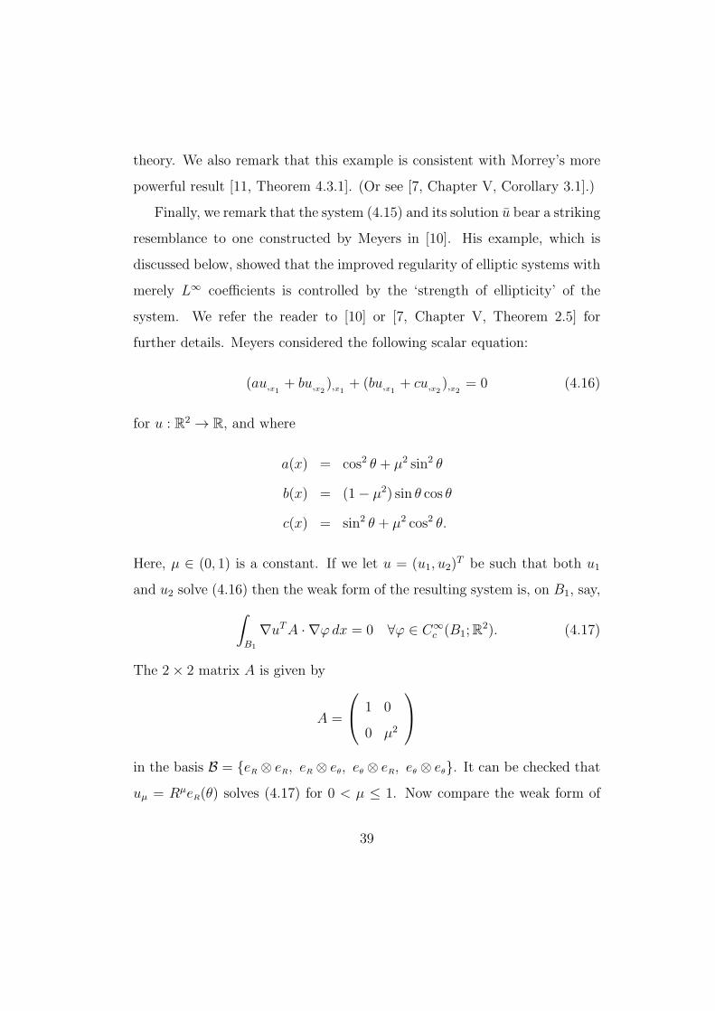
further details. Meyers considered the following scalar equation:

(au,x1 + bu,x2 ),x1 + (bu,x1 + cu,x2 ),x2 = 0 (4.16)

for u : R2 → R, and where

a(x) = cos2 θ + µ2 sin2 θ

b(x) = (1− µ2) sin θ cos θ

c(x) = sin2 θ + µ2 cos2 θ.

Here, µ ∈ (0, 1) is a constant. If we let u = (u1, u2)T be such that both u1

and u2 solve (4.16) then the weak form of the resulting system is, on B1, say,

∫

B1

∇uTA · ∇ϕdx = 0 ∀ϕ ∈ C∞c (B1;R

2). (4.17)

The 2× 2 matrix A is given by

A =

1 0

0 µ2

in the basis B = eR ⊗ eR, eR ⊗ eθ, eθ ⊗ eR, eθ ⊗ eθ. It can be checked that

uµ = RµeR(θ) solves (4.17) for 0 < µ ≤ 1. Now compare the weak form of

39

(4.15): in the same coordinate system it is

∫

Br

∇uA · ∇ϕdx = 0 ∀ϕ ∈ C∞c (B1;R

2),

where the 2× 2 matrix A is given by

A =

k2 0

0 1

.

We can see that Meyers used the same mechanism to ensure that a, b, c belong

to L∞(B1) \ C0(B1).

References

[1] J. Bevan. On one-homogeneous solutions to elliptic systems with spatial

variable dependence in two dimensions. Proceedings of the Royal Society

of Edinburgh: Section A Mathematics, 140 (2010), pp 449–475.

[2] R. Coifman, P.-L. Lions, Y. Meyer, and S. Semmes. Compensated com-

pactness and Hardy spaces. J. Math. Pures Appl. (9) 72 (1993), no. 3,

pp 247–286.

[3] B. Dacorogna. Direct methods in the calculus of variations. Second edi-

tion. Applied Mathematical Sciences, 78. Springer, New York, 2008.

[4] L. C. Evans and R. F. Gariepy. Measure theory and fine properties of

functions. Studies in Advanced Mathematics. CRC Press, Boca Raton,

FL, 1992.

[5] C. Fefferman and E. Stein. Hp spaces of several variables. Acta Math.

129 (1972), no. 3-4, 137–193.

40

[6] I. Fonseca and W. Gangbo. Degree theory in analysis and applications.

Oxford Lecture Series in Mathematics and its Applications, 2. Oxford

Science Publications. The Clarendon Press, Oxford University Press,

New York, 1995.

[7] M. Giaquinta. Multiple integrals in the calculus of variations and non-

linear elliptic systems. Annals of Mathematics Studies, 105. Princeton

University Press, Princeton, NJ, 1983.

[8] W. Hao, S. Leonardi and J. Necas. An example of irregular solution to a

nonlinear Euler-Lagrange elliptic system with real analytic coefficients.

Ann. Scuola Norm. Sup. Pisa Cl. Sci. (4) 23 (1996), no. 1, 57–67.

[9] R. Knops and C. Stuart. Quasiconvexity and uniqueness of equilibrium

solutions in nonlinear elasticity. Arch. Rational Mech. Anal. 86 (1984),

no. 3, 233–249.

[10] N. G. Meyers. An Lp-estimate for the gradient of solutions of second

order elliptic divergence equations. Ann. Scuola Norm. Sup. Pisa (3) 17

1963 189–206.

[11] C. B. Morrey. Multiple Integrals in the Calculus of Variations. Classics

in Mathematics, Springer, 2008.

[12] S. Muller and S. Spector. An existence theory for nonlinear elasticity

that allows for cavitation. Arch. Rational Mech. Anal. 131 (1995), no.

1, 1–66.

[13] S. Muller and V. Sverak. Convex integration for Lipschitz mappings

41

and counterexamples to regularity. Ann. of Math. (2) 157 (2003), no. 3,

715–742.

[14] J. Necas. Example of an irregular solution to a nonlinear elliptic sys-

tem with analytic coefficients and conditions for regularity. Theory of

nonlinear operators (Proc. Fourth Internat. Summer School, Acad. Sci.,

Berlin, 1975), pp. 197–206.

[15] D. Phillips. On one-homogeneous solutions to elliptic systems in two

dimensions. C. R. Math. Acad. Sci. Paris 335 (2002), no. 1, 39–42.

[16] R. T. Rockafellar. Convex Analysis. Princeton Landmarks in Mathemat-

ics and Physics, 1997.

[17] J. Sivaloganathan and S. Spector. On the symmetry of energy-

minimising deformations in nonlinear elasticity. I. Incompressible ma-

terials. Arch. Ration. Mech. Anal. 196 (2010), no. 2, 363–394.

[18] J. Sivaloganathan and S. Spector. On the symmetry of energy-

minimising deformations in nonlinear elasticity. II. Compressible ma-

terials. Arch. Ration. Mech. Anal. 196 (2010), no. 2, 395–431.

[19] E. Stein. Singular integrals and differentiability properties of functions.

Princeton University Press, 1970.

[20] V. Sverak. Regularity properties of deformations with finite energy.

Arch. Rational Mech. Anal. 100 (1988), no. 2, 105–127.

[21] V. Sverak and X. Yan. A singular minimizer of a smooth strongly convex

42

functional in three dimensions. Calc. Var. Partial Differential Equations

10 (2000), no. 3, 213–221.

[22] V. Sverak and X. Yan. Non-Lipschitz minimizers of smooth uniformly

convex functionals. Proc. Natl. Acad. Sci. USA 99 (2002), no. 24, 15269–

15276

[23] L. Szekelyhidi, Jr. The regularity of critical points of polyconvex func-

tionals. Arch. Ration. Mech. Anal. 172 (2004), no. 1, 133–152.

[24] M. Shahrokhi-Dehkordi and A. Taheri. Quasiconvexity and uniqueness

of stationary points on a space of measure preserving maps. J. Convex

Anal. 17 (2010), no. 1, 69–79.

[25] S.K. Vodopyanov and V.M. Goldstein. Quasiconformal mappings and

spaces of functions with generalized first derivatives. Siberian Math. J.

17 (No. 3) 1977, 515-531.

[26] W.P. Ziemer. Weakly differentiable functions. Graduate Texts in Math-

ematics, 120. Springer-Verlag, New York, 1989.

43