FMB - NLA

Block-tridiagonal matrices

. – p.1/31

FMB - NLA

Block-tridiagonal matrices - where do these arise?

- as a result of a particular mesh-point ordering

- as a part of a factorization procedure, for example when we compute

the eigenvalues of a matrix.

. – p.2/31

FMB - NLA Block-tridiagonal matrices

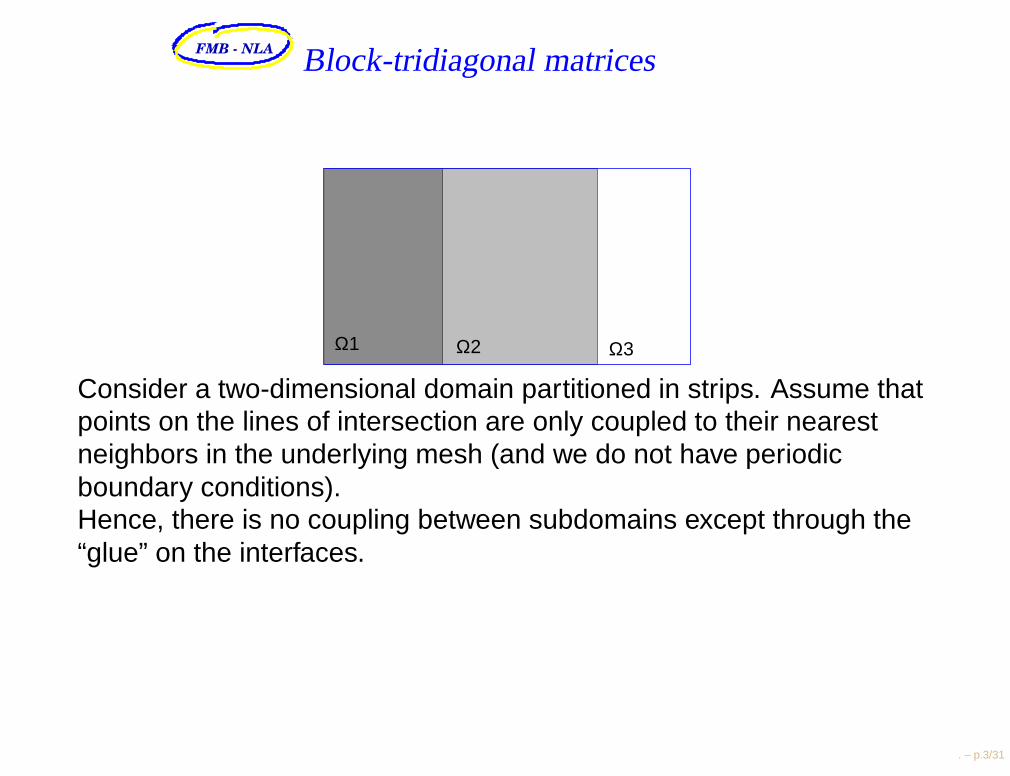
Ω1 Ω3Ω2

Consider a two-dimensional domain partitioned in strips. Assume thatpoints on the lines of intersection are only coupled to their nearestneighbors in the underlying mesh (and we do not have periodicboundary conditions).Hence, there is no coupling between subdomains except through the“glue” on the interfaces.

. – p.3/31

FMB - NLA Block-tridiagonal matrices

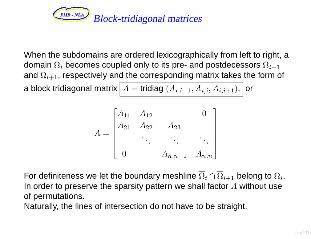
When the subdomains are ordered lexicographically from left to right, adomain Ωi becomes coupled only to its pre- and postdecessors Ωi1

and Ωi+1, respectively and the corresponding matrix takes the form of

a block tridiagonal matrix A = tridiag (Ai;i1; Ai;i; Ai;i+1), or

A =

266664A11 A12 0A21 A22 A23

. . .. . .

. . .

0 An;n1 An;n377775

For definiteness we let the boundary meshline Ωi \ Ωi+1 belong to Ωi.In order to preserve the sparsity pattern we shall factor A without useof permutations.Naturally, the lines of intersection do not have to be straight.

. – p.4/31

FMB - NLA Block-tridiagonal matrices

How do we factorize

a (block)-tridiagonal matrix ?

. – p.5/31

FMB - NLA

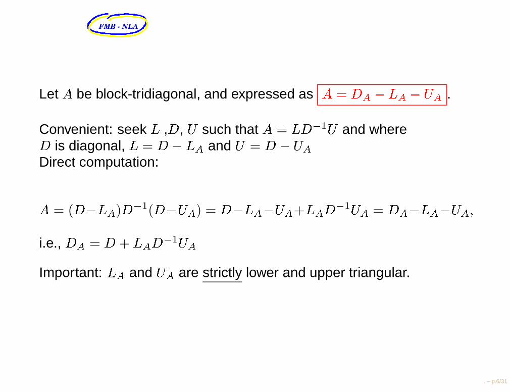
Let A be block-tridiagonal, and expressed as A = DA LA UA .

Convenient: seek L ,D, U such that A = LD1U and whereD is diagonal, L = D LA and U = D UADirect computation:

A = (DLA)D1(DUA) = DLAUA+LAD1UA = DALAUA;

i.e., DA = D + LAD1UAImportant: LA and UA are strictly lower and upper triangular.

. – p.6/31

FMB - NLA A = LD1U for pointwise tridiagonal matrices

2

6

6

6

6

6

6

4

a1;1 a2;2. . . an;n

3

7

7

7

7

7

7

5

=

2

6

6

6

6

6

6

4

d1 d2

. . . dn

3

7

7

7

7

7

7

5

+

2

6

6

6

6

6

6

4

0a2;1 0

. . .an;n1 0

3

7

7

7

7

7

7

5

2

6

6

6

6

6

6

4

1=d1

1=d2

. . .

1=dn3

7

7

7

7

7

7

5

2

6

6

6

6

6

6

4

0 a1;20 a2;3

. . .

0

3

7

7

7

7

7

7

5

Factorization algorithm:d1 = a1;1di = ai;i ai;i1ai1;idi1

. – p.7/31

FMB - NLA A = LD1U for pointwise tridiagonal matrices

Solution of systems with LD1U. – p.8/31

FMB - NLA Block-tridiagonal matrices

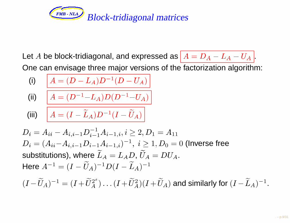
Let A be block-tridiagonal, and expressed as A = DA LA UA .

One can envisage three major versions of the factorization algorithm:

(i) A = (D LA)D1(D UA)

(ii) A = (D1LA)D(D1UA)

(iii) A = (I eLA)D1(I eUA)Di = Aii Ai;i1D1i1Ai1;i; i 2; D1 = A11Di = (AiiAi;i1Di1Ai1;i)1; i 1; D0 = 0 (Inverse free

substitutions), where eLA = LAD, eUA = DUA.Here A1 = (I eUA)1D(I eLA)1

(I eUA)1 = (I+ eU2sA ) : : : (I+ eU2A)(I+ eUA) and similarly for (I eLA)1.

. – p.9/31

FMB - NLA Existence of factorization for block-tridiagonal matrices

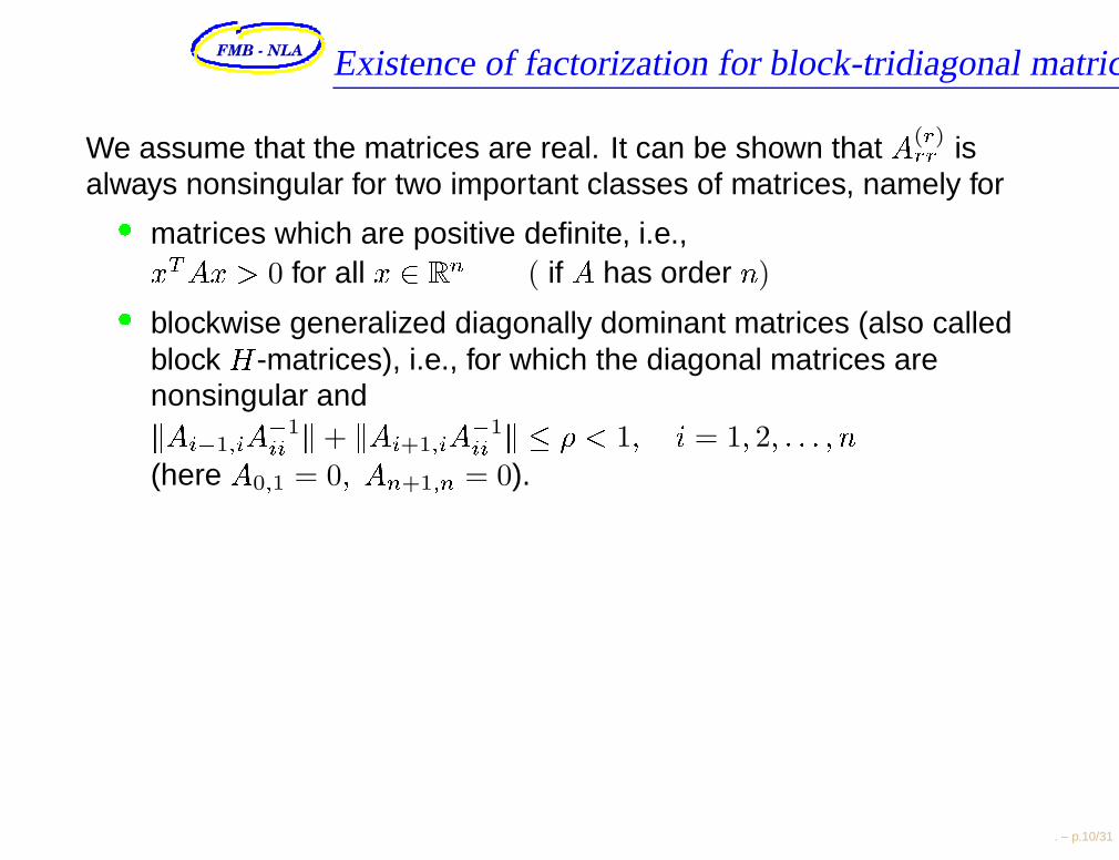
We assume that the matrices are real. It can be shown that A(r)rr isalways nonsingular for two important classes of matrices, namely for matrices which are positive definite, i.e.,xTAx > 0 for all x 2 R n ( if A has order n) blockwise generalized diagonally dominant matrices (also called

block H-matrices), i.e., for which the diagonal matrices arenonsingular andkAi1;iA1ii k + kAi+1;iA1ii k < 1; i = 1; 2; : : : ; n(here A0;1 = 0; An+1;n = 0).

. – p.10/31

FMB - NLA A factorization passes through stages r = 1; 2; : : : ; n 1

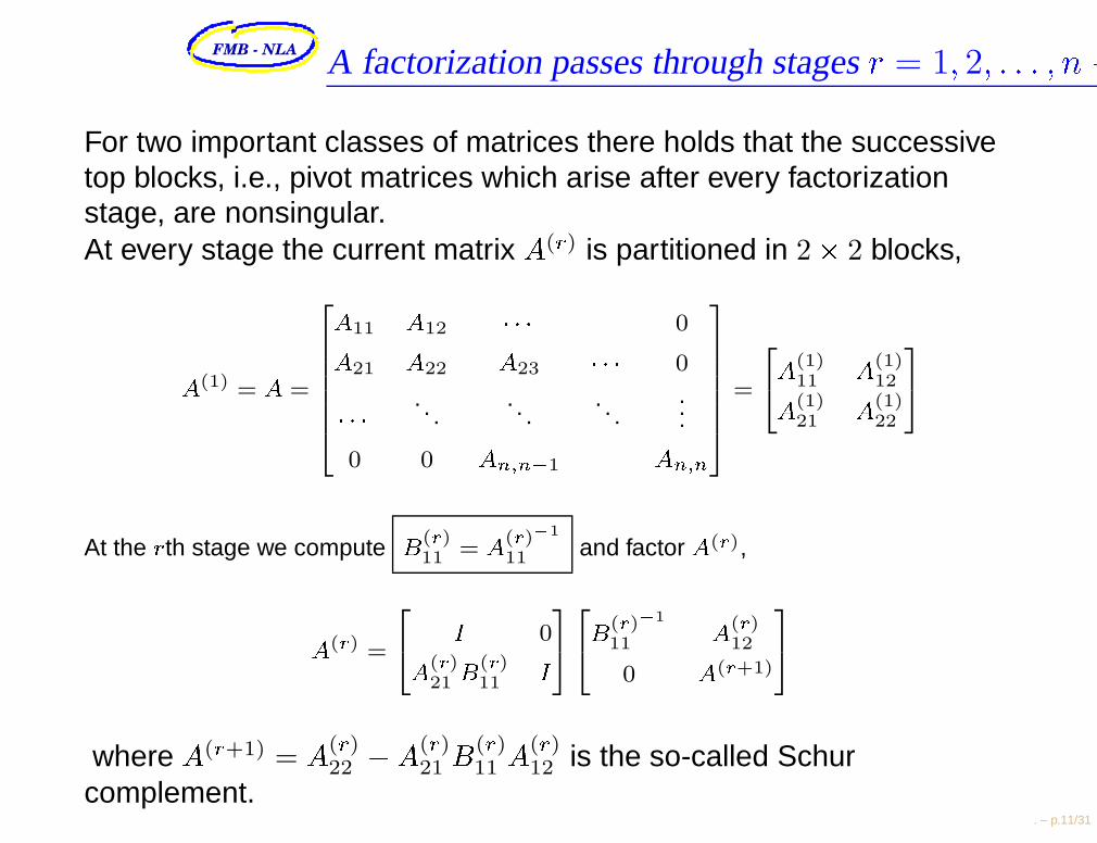
For two important classes of matrices there holds that the successivetop blocks, i.e., pivot matrices which arise after every factorizationstage, are nonsingular.At every stage the current matrix A(r) is partitioned in 2 2 blocks,

A(1) = A =

2

6

6

6

6

6

6

4

A11 A12 0A21 A22 A23 0 . . .. . .

. . ....

0 0 An;n1 An;n3

7

7

7

7

7

7

5

=

2

4

A(1)11 A(1)

12A(1)21 A(1)

22

3

5

At the rth stage we compute B(r)11 = A(r)1

11 and factor A(r),

A(r) =

2

4

I 0A(r)21 B(r)

11 I3

5

2

4

B(r)1

11 A(r)12

0 A(r+1)

3

5

where A(r+1) = A(r)22 A(r)

21 B(r)11 A(r)

12 is the so-called Schurcomplement.

. – p.11/31

FMB - NLA Existence of factorization for block-tridiagonal matrices

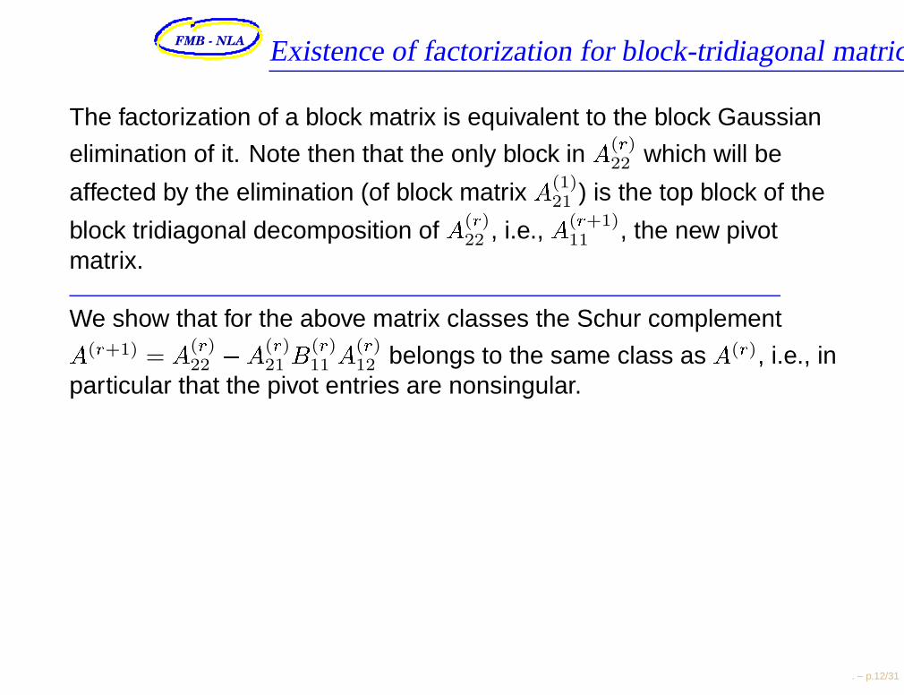
The factorization of a block matrix is equivalent to the block Gaussian

elimination of it. Note then that the only block in A(r)22 which will be

affected by the elimination (of block matrix A(1)21 ) is the top block of the

block tridiagonal decomposition of A(r)22 , i.e., A(r+1)

11 , the new pivotmatrix.

We show that for the above matrix classes the Schur complementA(r+1) = A(r)22 A(r)

21 B(r)11 A(r)

12 belongs to the same class as A(r), i.e., inparticular that the pivot entries are nonsingular.

. – p.12/31

FMB - NLA

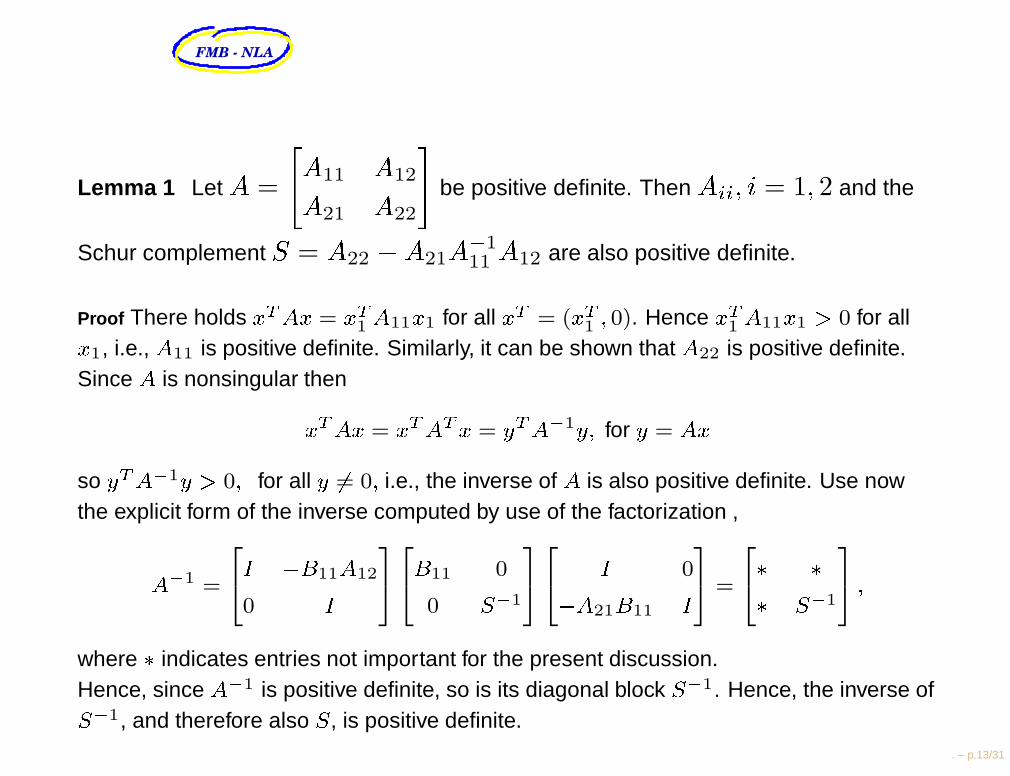
Lemma 1 Let A =

"A11 A12A21 A22

#

be positive definite. Then Aii; i = 1; 2 and the

Schur complement S = A22 A21A111 A12 are also positive definite.

Proof There holds xTAx = xT1 A11x1 for all xT = (xT1 ; 0). Hence xT1 A11x1 > 0 for allx1, i.e., A11 is positive definite. Similarly, it can be shown that A22 is positive definite.Since A is nonsingular thenxTAx = xTATx = yTA1y; for y = Axso yTA1y > 0; for all y 6= 0; i.e., the inverse of A is also positive definite. Use nowthe explicit form of the inverse computed by use of the factorization ,A1 =

2

4

I B11A12

0 I 3

5

2

4

B11 0

0 S1

3

5

2

4

I 0A21B11 I3

5 =

2

4

S1

3

5 ;

where indicates entries not important for the present discussion.Hence, since A1 is positive definite, so is its diagonal block S1. Hence, the inverse ofS1, and therefore also S, is positive definite.

. – p.13/31

FMB - NLA

Corollary 1 When A(r) is positive definite, A(r+1) and in particular, A(r+1)11 are

positive definite.

Proof A(r+1) is a Schur complement of A(r) so by Lemma 1, A(r+1)

is positive definite when A(r) is. In particular, its top diagonal block is

positive definite.

. – p.14/31

FMB - NLA

Lemma 2 Let A =

"A11 A12A21 A22

#

be blockwise generalized diagonally dominant

where A is block tridiagonal. Then the Schur complement S = A22 A21A111 A12

is also generalized diagonally dominant.

Proof (Hint) Since the only matrix block in S which has been changed

from A22 is its top block B11 to A(r+1)11 it suffices to show that A11 is non-

singular and the first block column is generalized diagonally dominant.

. – p.15/31

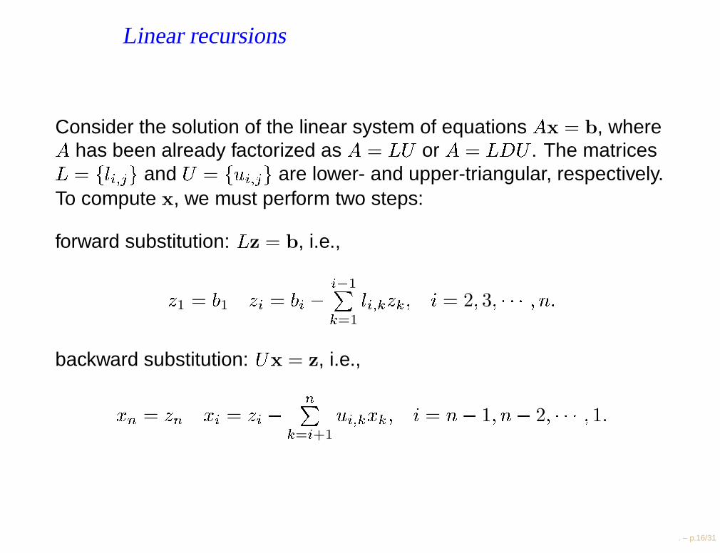
Linear recursions

Consider the solution of the linear system of equations Ax = b, whereA has been already factorized as A = LU or A = LDU . The matricesL = fli;jg and U = fui;jg are lower- and upper-triangular, respectively.To compute x, we must perform two steps:

forward substitution: Lz = b, i.e.,

z1 = b1 zi = bi i1Pk=1

li;kzk; i = 2; 3; ; n:

backward substitution: Ux = z, i.e.,xn = zn xi = zi nPk=i+1

ui;kxk; i = n 1; n 2; ; 1:

. – p.16/31

FMB - NLA

While the implementation of the forward and back-substitution on aserial computer is trivial, to implement them on a vector or parallelcomputer system is problematic. The reason is that the relations areparticular examples of a linear recursion which is an inherentlysequential process. A general m-level recurrence relation reads asxi = a1;ixi1 + a2;ixi2 + + am;ixim + bi;

and the performance of its straightforward vector or parallelimplementation is degraded due to the existing backwards datadependencies.

. – p.17/31

FMB - NLA Block-tridiagonal matrices

Can we speedup somehow

the solution of systems

with bi- or tri-diagonal matrices ?

. – p.18/31

FMB - NLA Multifrontal solution methods

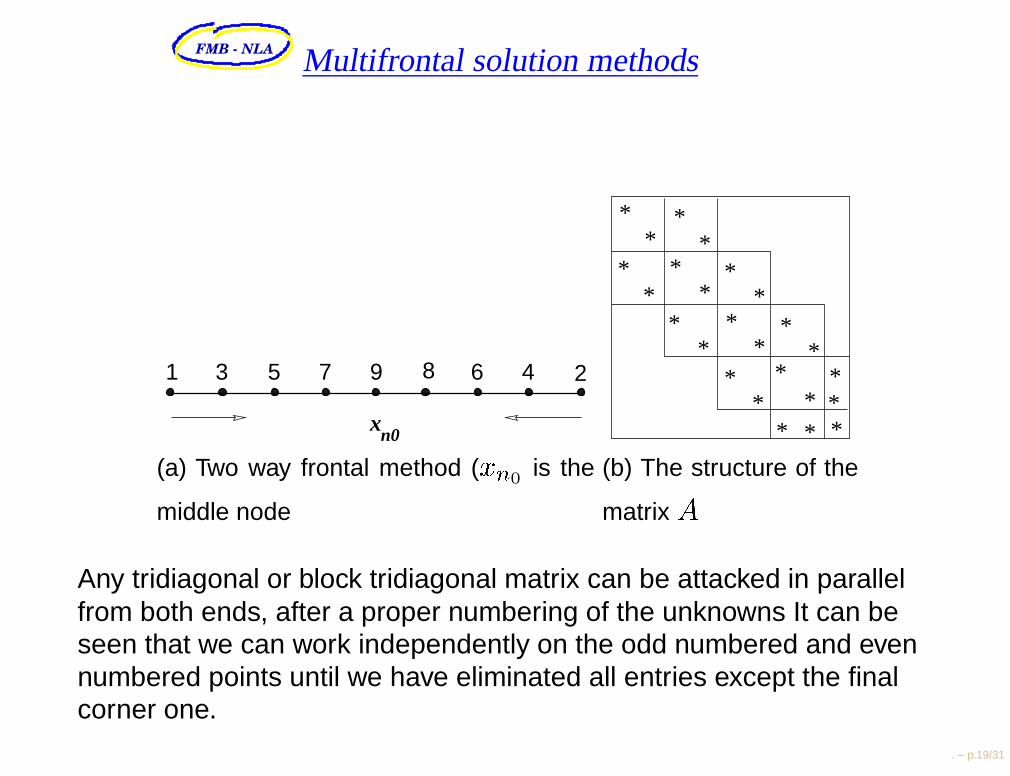
1 3 5 7 9 8 6 4 2

xn0

(a) Two way frontal method (xn0 is the

middle node

**

**

**

**

***

**

**

**

**

**

**

**

(b) The structure of the

matrix A

Any tridiagonal or block tridiagonal matrix can be attacked in parallelfrom both ends, after a proper numbering of the unknowns It can beseen that we can work independently on the odd numbered and evennumbered points until we have eliminated all entries except the finalcorner one.

. – p.19/31

FMB - NLA

Hence, the factorization and forward substitution can occur in parallelfor the two fronts (the even and the odd).At the final point we can either continue in parallel with the backsubstitution to compute the solution at all the other interior points, orwe can use the same type of two way frontal method now for each ofthe two structures which have been split by the already computedsolution at the middle point.

This method of recursively dividing the domain in smaller and smallerpieces which can be handled all in parallel, can be continued dlog2 ne

steps, after which we have just one unknown per subinterval.

. – p.20/31

FMB - NLA

The idea to perform Gaussian elimination from both ends of atridiagonal matrix, called also twisted factorization, was proposed firstby Babushka in 1972.

Note that in this method no back substitution is required.

. – p.21/31

FMB - NLA Odd-even elimination/cyclic reduction/divide-

and-conquer

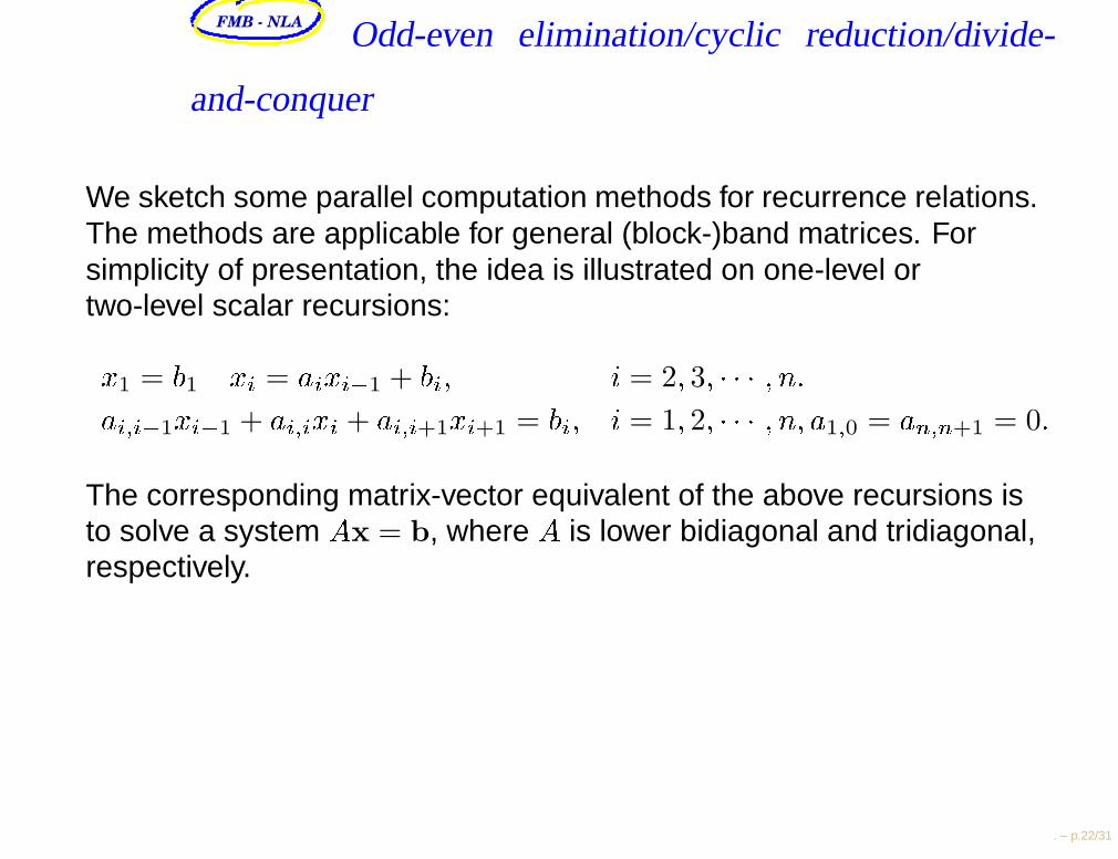
We sketch some parallel computation methods for recurrence relations.The methods are applicable for general (block-)band matrices. Forsimplicity of presentation, the idea is illustrated on one-level ortwo-level scalar recursions:x1 = b1 xi = aixi1 + bi; i = 2; 3; ; n:ai;i1xi1 + ai;ixi + ai;i+1xi+1 = bi; i = 1; 2; ; n; a1;0 = an;n+1 = 0:

The corresponding matrix-vector equivalent of the above recursions isto solve a system Ax = b, where A is lower bidiagonal and tridiagonal,respectively.

. – p.22/31

FMB - NLA

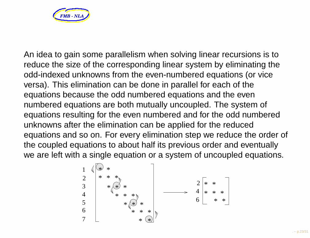
An idea to gain some parallelism when solving linear recursions is toreduce the size of the corresponding linear system by eliminating theodd-indexed unknowns from the even-numbered equations (or viceversa). This elimination can be done in parallel for each of theequations because the odd numbered equations and the evennumbered equations are both mutually uncoupled. The system ofequations resulting for the even numbered and for the odd numberedunknowns after the elimination can be applied for the reducedequations and so on. For every elimination step we reduce the order ofthe coupled equations to about half its previous order and eventuallywe are left with a single equation or a system of uncoupled equations.

642

**

**

234

67

1

* * ** * *

* * ** * *

* * ** *

5

* *

**

*

. – p.23/31

FMB - NLA

In the odd-even elimination (or odd-even reduction) method weeliminate the odd numbered unknowns (i.e., numbers 1 (mod 2)) andwe are left with a tridiagonal system for the even numbered (i.e.,numbers 2 (mod 2)) unknowns. The method is repeated, i.e., weeliminate the unknowns 2 (mod 4) and are left with the unknownsnumbered 4 (mod 4) and so on. Eventually we are left with just a singleequation which we solve. At this point we can use back substitution tocompute the remaining unknowns.

. – p.24/31

FMB - NLA ...the odd-even simultaneous ...

There exist a second version of this method, called the odd-evensimultaneous elimination. In the odd-even simultaneous eliminationmethod we eliminate the odd-numbered unknowns from the evennumbered equations and simultaneously the even numberedunknowns from the odd equations. In this way we are left with twodecoupled equations, one for the even numbered unknowns and onefor the odd numbered unknowns. The same method can be recursivelyapplied for these two sets in parallel.

Hence, in this method we do not reduce the size of the problem but wesuccessively decouple the problems into smaller and smaller sizes ofsubproblems. Eventually we arrive at a system on diagonal form whichwe solve for all unknowns in parallel. Therefore, in this method there isno need to perform back substitution.

. – p.25/31

FMB - NLA ...the odd-even...

4627351

8642753

8

1

8

**

*

* **

*

*

**

*

* **

*

*

*

*

* ** * *

*

*

*

*

234

67

1

5 *

**

* * ** * *

* * ** * *

*****

*****

***

*

*

*

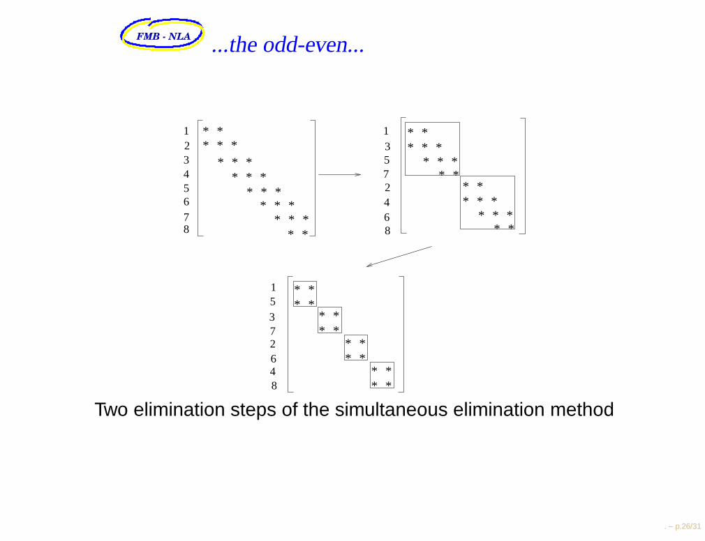
Two elimination steps of the simultaneous elimination method

. – p.26/31

FMB - NLA ...the odd-even...

The computational complexity of the sequential LU factorization andforward and back substitution method for three-diagonal matrices is 8n.

While performing the odd-even simultaneous elimination we perform9ndlog2 ne flops to transform the system and n flops to solve the lastdiagonal system.

Hence, the redundancy of the odd-even simultaneous eliminationmethod is 9=8dlog2 ne which is the price we pay to get a fully parallelmethod.

. – p.27/31

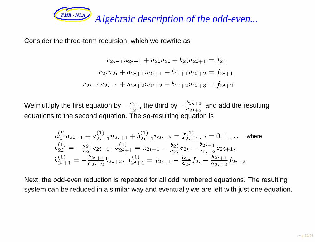
FMB - NLA Algebraic description of the odd-even...

Consider the three-term recursion, which we rewrite as 2i1u2i1 + a2iu2i + b2iu2i+1 = f2i 2iu2i + a2i+1u2i+1 + b2i+1u2i+2 = f2i+1 2i+1u2i+1 + a2i+2u2i+2 + b2i+2u2i+3 = f2i+2

We multiply the first equation by 2ia2i , the third by b2i+1a2i+2and add the resulting

equations to the second equation. The so-resulting equation is (i)2i u2i1 + a(1)

2i+1u2i+1 + b(1)2i+1u2i+3 = f (1)

2i+1; i = 0; 1; : : : where (1)2i = 2ia2i 2i1; a(1)

2i+1 = a2i+1 b2ia2i 2i b2i+1a2i+2

2i+1;b(1)2i+1 = b2i+1a2i+2

b2i+2; f (1)2i+1 = f2i+1 2ia2i f2i b2i+1a2i+2

f2i+2

Next, the odd-even reduction is repeated for all odd numbered equations. The resultingsystem can be reduced in a similar way and eventually we are left with just one equation.

. – p.28/31

FMB - NLA

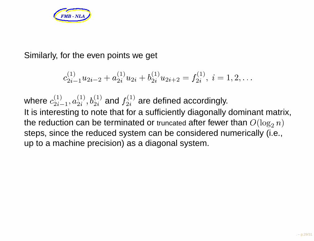
Similarly, for the even points we get (1)2i1u2i2 + a(1)

2i u2i + b(1)2i u2i+2 = f (1)

2i ; i = 1; 2; : : :where (1)

2i1; a(1)2i ; b(1)

2i and f (1)2i are defined accordingly.

It is interesting to note that for a sufficiently diagonally dominant matrix,the reduction can be terminated or truncated after fewer than O(log2 n)steps, since the reduced system can be considered numerically (i.e.,up to a machine precision) as a diagonal system.

. – p.29/31

FMB - NLA

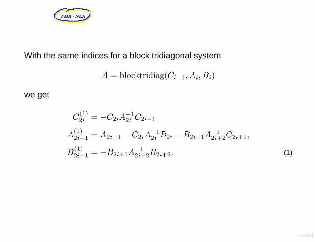
With the same indices for a block tridiagonal systemA = blocktridiag(Ci1; Ai; Bi)we get C(1)

2i = C2iA12i C2i1A(1)

2i+1 = A2i+1 C2iA12i B2i B2i+1A1

2i+2C2i+1;B(1)2i+1 = B2i+1A1

2i+2B2i+2: (1)

. – p.30/31

FMB - NLA Some keywords to discuss

Load balancing for cyclic reduction methods Divide-and-conquer techniques Domain decomposition ordering

. – p.31/31