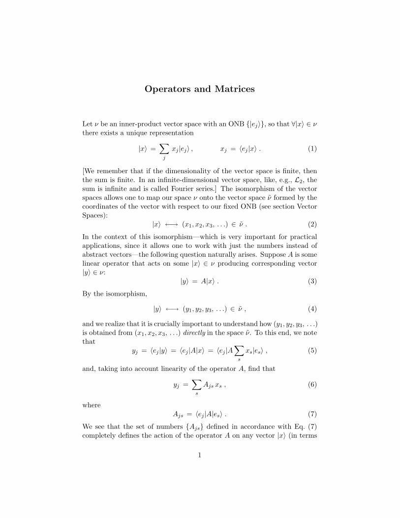
Operators and Matrices

Let ν be an inner-product vector space with an ONB {|ej〉}, so that ∀|x〉 ∈ νthere exists a unique representation

|x〉 =∑

j

xj |ej〉 , xj = 〈ej |x〉 . (1)

[We remember that if the dimensionality of the vector space is finite, thenthe sum is finite. In an infinite-dimensional vector space, like, e.g., L2, thesum is infinite and is called Fourier series.] The isomorphism of the vectorspaces allows one to map our space ν onto the vector space ν formed by thecoordinates of the vector with respect to our fixed ONB (see section VectorSpaces):

|x〉 ←→ (x1, x2, x3, . . .) ∈ ν . (2)

In the context of this isomorphism—which is very important for practicalapplications, since it allows one to work with just the numbers instead ofabstract vectors—the following question naturally arises. Suppose A is somelinear operator that acts on some |x〉 ∈ ν producing corresponding vector|y〉 ∈ ν:

|y〉 = A|x〉 . (3)

By the isomorphism,

|y〉 ←→ (y1, y2, y3, . . .) ∈ ν , (4)

and we realize that it is crucially important to understand how (y1, y2, y3, . . .)is obtained from (x1, x2, x3, . . .) directly in the space ν. To this end, we notethat

yj = 〈ej |y〉 = 〈ej |A|x〉 = 〈ej |A∑

s

xs|es〉 , (5)

and, taking into account linearity of the operator A, find that

yj =∑

s

Ajs xs , (6)

whereAjs = 〈ej |A|es〉 . (7)

We see that the set of numbers {Ajs} defined in accordance with Eq. (7)completely defines the action of the operator A on any vector |x〉 (in terms

1

of the coordinates with respect to a given ONB). This set of numbers iscalled matrix of the operator A with respect to the given ONB. If the ONBis fixed or at least is not being explicitly changed, then it is convenient to usethe same letter A for both operator A and its matrix (with respect to ourONB). Each particular element Ajs (say, A23) is called matrix element ofthe operator A (with respect to the given ONB). In Mathematics, by matrixone means a two-subscript set of numbers (normally represented by a table,which, however is not necessary, and not always convenient) with a ceratinrules of matrix addition, multiplication of a matrix by a number, and matrixmultiplication. These rules, forming matrix algebra, are naturally derivablefrom the properties of linear operators in the vector spaces which, as wehave seen above, can be represented by matrices. Let us derive these rules.

Addition. The sum, C = A + B, of two operators, A and B, is naturallydefined as an operator that acts on vectors as follows.

C|x〉 = A|x〉 + B|x〉 . (8)

Correspondingly, the matrix elements of the operator C = A + B are givenby

Cij = Aij + Bij , (9)

and this is exactly how a sum of two matrices is defined in matrix theory.Multiplication by a number. The product B = λA of a number λ and an

operator A is an operator that acts as follows.

B|x〉 = λ(A|x〉) . (10)

The product C = Aλ of an operator A and a number λ is an operator thatacts as follows.

C|x〉 = A(λ|x〉) . (11)

If A is a linear operator (which we will be assuming below), then B = C,and we do not need to pay attention to the order in which the number andthe operator enter the product. Clearly, corresponding matrix is

Cij = Bij = λAij , (12)

and this is how a product of a number and a matrix is defined in the theoryof matrices.

Multiplication. The product, C = AB, of two operators, A and B, isdefined as an operator that acts on vectors as follows

C|x〉 = A(B|x〉) . (13)

2

That is the rightmost operator, B, acts first, and then the operator A actson the vector resulting from the action of the operator B.

The operator multiplication is associative: for any three operators A, B,and C, we have A(BC) = (AB)C. But the operator multiplication is notcommutative: generally speaking, AB 6= BA.

It is easy to check that the matrix elements of the operator C = AB aregiven by

Cij =∑

s

AisBsj . (14)

And this is exactly how a product of two matrices is defined in matrix theory.Each linear operator is represented by corresponding matrix, and the

opposite is also true: each matrix generates corresponding linear operator.Previously we introduced the notion of an adjoint (Hermitian conjugate)

operator (see Vector Spaces chapter). The operator A† is adjoint to A if∀ |x〉, |y〉 ∈ ν

〈y|Ax〉 = 〈A†y|x〉 = 〈x|A†y〉 . (15)

Expanding |x〉 and |y〉 in terms of our ONB, one readily finds that

〈y|Ax〉 =∑

ij

Aij y∗i xj , (16)

〈x|A†y〉 =∑

ij

(A†ji)∗ xjy

∗i , (17)

and, taking into account that Eq. (15) is supposed to take place for any |x〉and |y〉, concludes that

A†ji = A∗ij . (18)

We see that the matrix of an operator adjoint to a given operator A isobtained from the matrix A by interchanging the subscripts and complexconjugating. In the matrix language, the matrix which is obtained froma given matrix A by interchanging the subscripts is called transpose of Aand is denoted as AT. By a complex conjugate of the matrix A (denotedas A∗) one understands the matrix each element of which is obtained fromcorresponding element of A by complex conjugation. Speaking this language,the matrix of the adjoint operator is a complex conjugate transpose of thematrix of the original operator. They also say that the matrix A† is theHermitian conjugate of the matrix A. In fact, all the terminology applicableto linear operators is automatically applicable to matrices, because of theabove-established isomorphism between these two classes of objects.

3

For a self-adjoint (Hermitian) operator we have

A = A† ⇔ Aji = A∗ij . (19)

Corresponding matrices are called Hermitian. There are also anti-Hermitianoperators and matrices:

A = −A† ⇔ −Aji = A∗ij . (20)

There is a close relationship between Hermitian and anti-Hermitian opera-tors/matrices. If A is Hermitian, then iA is anti-Hermitian, and vice versa.

An identity operator, I, is defined as

I|x〉 = |x〉 . (21)

Correspondingly,Iij = δij . (22)

It is worth noting that an identity operator can be non-trivially written asthe sum over projectors onto the basis vectors:

I =∑

j

|ej〉〈ej | . (23)

Equation (23) is also known as the completeness relation for the orthonormalsystem {|ej〉}, ensuring that it forms a basis. For an incomplete orthonormalsystem, corresponding operator is not equal to the identity operator. [Itprojects a vector onto the sub-space of vectors spanned by this ONS.]

In a close analogy with the idea of Eq. (23), one can write a formulaexplicitly restoring an operator from its matrix in terms of the operationsof inner product and multiplication of a vector by a number:

A =∑

ij

|ei〉Aij〈ej | . (24)

Problem 26. The three 2× 2 matrices, A, B, and C, are defined as follows.

A12 = A21 = 1 , A11 = A22 = 0 , (25)

−B12 = B21 = i , B11 = B22 = 0 , (26)

C12 = C21 = 0 , C11 = −C22 = 1 . (27)

4

Represent these matrices as 2× 2 tables. Make sure that (i) all the three matricesare Hermitian, and (ii) feature the following properties.

AA = BB = CC = I , (28)

BC = iA , CA = iB , AB = iC , (29)

CB = −iA , AC = −iB , BA = −iC . (30)

For your information. Matrices A, B, and C are the famous Pauli matrices. InQuantum Mechanics, these matrices and the above relations between them play acrucial part in the theory of spin.

Problem 27. Show that:(a) For any two linear operators A and B, it is always true that (AB)† = B†A†.(b) If A and B are Hermitian, the operator AB is Hermitian only when AB = BA.(c) If A and B are Hermitian, the operator AB −BA is anti-Hermitian.

Problem 28. Show that under canonical boundary conditions the operator A =∂/∂x is anti-Hermitian. Then make sure that for the operator B defined as B|f〉 =xf(x) (that is the operator B simply multiplies any function f(x) by x) and forthe above-defined operator A the following important commutation relation takesplace

AB − BA = I . (31)

Problem 29. In the Hilbert space L2[−1, 1], consider a subspace spanned by thefollowing three vectors.

e1(x) =1√2

, (32)

e2(x) =1√2

(sin

π

2x + cos πx

), (33)

e3(x) =1√2

(sin

π

2x − cos πx

). (34)

(a) Make sure that the three vectors form an ONB in the space spanned by them(that is show that they are orthogonal and normalized).(b) Find matrix elements of the Laplace operator B = ∂2/∂x2 in this ONB. Makesure that the matrix B is Hermitian.

5

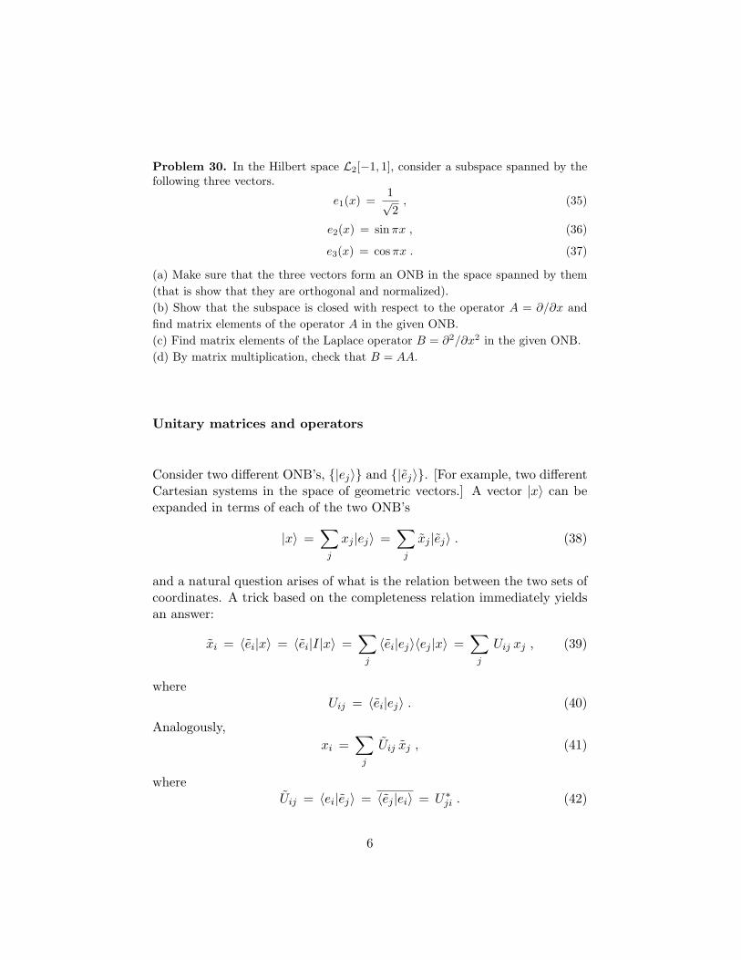
Problem 30. In the Hilbert space L2[−1, 1], consider a subspace spanned by thefollowing three vectors.

e1(x) =1√2

, (35)

e2(x) = sin πx , (36)

e3(x) = cos πx . (37)

(a) Make sure that the three vectors form an ONB in the space spanned by them(that is show that they are orthogonal and normalized).(b) Show that the subspace is closed with respect to the operator A = ∂/∂x andfind matrix elements of the operator A in the given ONB.(c) Find matrix elements of the Laplace operator B = ∂2/∂x2 in the given ONB.(d) By matrix multiplication, check that B = AA.

Unitary matrices and operators

Consider two different ONB’s, {|ej〉} and {|ej〉}. [For example, two differentCartesian systems in the space of geometric vectors.] A vector |x〉 can beexpanded in terms of each of the two ONB’s

|x〉 =∑

j

xj |ej〉 =∑

j

xj |ej〉 . (38)

and a natural question arises of what is the relation between the two sets ofcoordinates. A trick based on the completeness relation immediately yieldsan answer:

xi = 〈ei|x〉 = 〈ei|I|x〉 =∑

j

〈ei|ej〉〈ej |x〉 =∑

j

Uij xj , (39)

whereUij = 〈ei|ej〉 . (40)

Analogously,xi =

∑

j

Uij xj , (41)

whereUij = 〈ei|ej〉 = 〈ej |ei〉 = U∗

ji . (42)

6

We arrive at an important conclusion that the transformation of coordinatesof a vector associated with changing the basis formally looks like the actionof a linear operator on the coordinates treated as vectors from ν. Thematrix of the operator that performs the transformation {xj} → {xj} is U ,the matrix elements being defined by (40). The matrix of the operator thatperforms the transformation {xj} → {xj} is U , the matrix elements beingdefined by (42). Eq. (42) demonstrates that the two matrices are related toeach other through the procedure of Hermitian conjugation:

U = U † , U = U † . (43)

Since the double transformations {xj} → {xj} → {xj} and {xj} → {xj} →{xj} are, by construction, just identity transformations, we have

UU = I , UU = I . (44)

Then, with Eq. (43) taken into account, we get

U †U = I , UU † = I . (45)

The same is automatically true for U = U †, which plays the same role as U .The matrices (operators) that feature the property (45) are termed unitarymatrices (operators).

One of the most important properties of unitary operators, implied byEq. (45), is that ∀ |x〉, |y〉 ∈ ν we have

〈Ux |Uy 〉 = 〈x | y 〉 . (46)

In words, a unitary transformation of any two vectors does not change theirinner product. This fact has a very important immediate corollary. If wetake in (46), |x〉 = |ei〉, |y〉 = |ej〉 and denote the transformed vectorsaccording to U |x〉 = |li〉, U |y〉 = |lj〉, we obtain

〈 li | lj 〉 = 〈Uei |Uej 〉 = 〈 ei | ej 〉 = δi j , (47)

meaning that an ONB {|ei〉} is transformed by U into another ONB, {|li〉}.Note, that in two- and three-dimensional real-vector spaces, (47) impliesthat U can only consist of rotations of the basis as a whole and flips of someof the resulting vectors into the opposite direction (mirror reflections). A bitjargonically, they say that the operator U rotates the vectors of the originalspace ν.

So far, we were dealing with the action of the matrix U in the vectorspace ν of the coordinates of our vectors. Let us now explore the action

7

of corresponding operator U in the original vector space ν. To this end weformally restore the operator from its matrix by Eq. (24):

U =∑

ij

|ei〉Uij〈ej | =∑

ij

|ei〉〈ei|ej〉〈ej | . (48)

Now using the completeness relation (23), we arrive at the most elegantexpression

U =∑

i

|ei〉〈ei| , (49)

from which it is directly seen that

U |ei〉 = |ei〉 . (50)

That is the operator U takes the i-th vector of the new basis and transformsit into the i-th vector of the old basis.

Note an interesting subtlety: in terms of the coordinates—as opposed tothe basis vectors, the matrix U is responsible for transforming old coordi-nates into the new ones.

Clearly, the relations for the matrix/operator U are identical, up tointerchanging tilded and non-tilde quantities.

Any unitary operator U acting in the vector space ν can be constructedby its action on some ONB {|ei〉}. In view of the property (47), this trans-formation will always produce an ONB and will have a general form of (50).Hence, we can write down the transformation {|ei〉} → {|ei〉} explicitly as

U |ei〉 = |ei〉 ⇐⇒ U =∑

i

|ei〉〈ei| . (51)

Applying the identity operator I =∑

j |ej〉〈ej | to the left hand side of thefirst equation, we arrive at the expansion of the new basis in terms of theold one

|ei〉 =∑

j

Uji |ej〉, (52)

where the matrix Uij is given by

Uij = 〈ei|U |ej〉 = 〈ei|ej〉 . (53)

(Compare to Eq. (40).) Thus, for any vector |x〉 transformed by U , itscoordinates in the basis {|ei〉} are transformed according to

x′i =∑

j

Uij xj . (54)

8

Note that, in contrast to (39), {xi} and {x′i} are the coordinates of theoriginal vector and the “rotated” one in the same basis {|ei〉}. Interestingly,since the coordinates of the vector |ej〉 itself are xk = 0 for all k exceptk = j, xj = 1, the matrix element Uij is nothing but the i-th coordinateof the transform of |ej〉. The latter property can be also used to explicitlyconstruct Uij .

Rotations in real-vector spaces

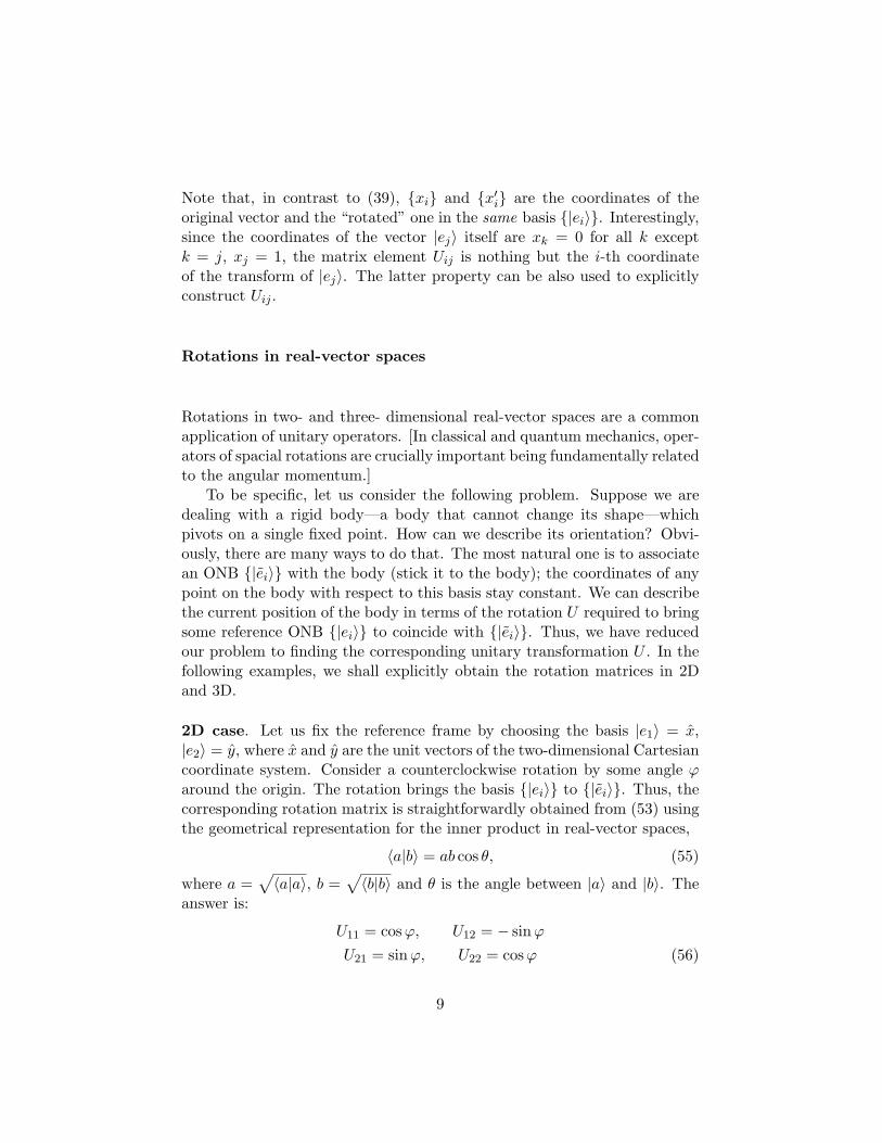
Rotations in two- and three- dimensional real-vector spaces are a commonapplication of unitary operators. [In classical and quantum mechanics, oper-ators of spacial rotations are crucially important being fundamentally relatedto the angular momentum.]

To be specific, let us consider the following problem. Suppose we aredealing with a rigid body—a body that cannot change its shape—whichpivots on a single fixed point. How can we describe its orientation? Obvi-ously, there are many ways to do that. The most natural one is to associatean ONB {|ei〉} with the body (stick it to the body); the coordinates of anypoint on the body with respect to this basis stay constant. We can describethe current position of the body in terms of the rotation U required to bringsome reference ONB {|ei〉} to coincide with {|ei〉}. Thus, we have reducedour problem to finding the corresponding unitary transformation U . In thefollowing examples, we shall explicitly obtain the rotation matrices in 2Dand 3D.

2D case. Let us fix the reference frame by choosing the basis |e1〉 = x,|e2〉 = y, where x and y are the unit vectors of the two-dimensional Cartesiancoordinate system. Consider a counterclockwise rotation by some angle ϕaround the origin. The rotation brings the basis {|ei〉} to {|ei〉}. Thus, thecorresponding rotation matrix is straightforwardly obtained from (53) usingthe geometrical representation for the inner product in real-vector spaces,

〈a|b〉 = ab cos θ, (55)

where a =√〈a|a〉, b =

√〈b|b〉 and θ is the angle between |a〉 and |b〉. The

answer is:

U11 = cosϕ, U12 = − sinϕ

U21 = sinϕ, U22 = cosϕ (56)

9

3D case. In three dimensions, the situation is more complicated. Apartfrom special cases, the direct approach using Eqs. (53),(55) is rather incon-venient. To start with, one can wonder how many variables are necessary todescribe an arbitrary rotation. The answer is given by the Euler’s rotationtheorem, which claims that an arbitrary rotation in three dimensions canbe represented by only three parameters. We shall prove the theorem byexplicitly obtaining these parameters.

The idea is to represent an arbitrary rotation by three consecutive simplerotations (the representation is not unique and we shall use one of the mostcommon). Here, by a simple rotation we mean a rotation around one of theaxes of the Cartesian coordinate system. For example, the matrix of rotationaround the z-axis by angle α, Aij(α), is easily obtained by a generalizationof (56). We just have to note that the basis vector |e3〉 = z is unchangedby such rotation—it is an eigenvector of the rotation operator with theeigenvalue 1. Thus, Eq. (52) implies that A13 = A23 = A31 = A32 = 0 andA33 = 1. Clearly, the remaining components coincide with those of Uij in(56), so for Aij(α) we get

A11 = cosα, A12 = − sinα, A13 = 0,

A21 = sin α, A22 = cosα, A23 = 0,

A31 = 0, A32 = 0, A33 = 1. (57)

The convention for the sign of α is such that α is positive if the rotationobserved along the vector −z is counterclockwise. We shall also need arotation around the x-axis, Bij(β), which by analogy with (57) is given by

B11 = 1, B12 = 0, B13 = 0,

B21 = 0, B22 = cosβ, B23 = − sinβ,

B31 = 0, B32 = sin β, B33 = cosβ. (58)

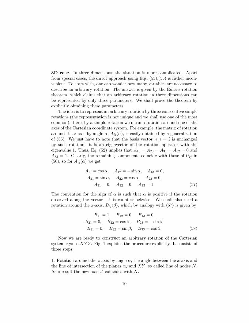
Now we are ready to construct an arbitrary rotation of the Cartesiansystem xyz to XY Z. Fig. 1 explains the procedure explicitly. It consists ofthree steps:

1. Rotation around the z axis by angle α, the angle between the x-axis andthe line of intersection of the planes xy and XY , so called line of nodes N .As a result the new axis x′ coincides with N .

10

2. Rotation around N (the x′ axis) by angle β, the angle between z and Z.As a result the axis z coincides with Z.

3. Rotation around Z ≡ z by angle γ, the angle between N and X, whichfinally brings the coordinate systems together.

Figure 1: Rotation in 3D. Euler angles.

The angles α, β, γ are the famous Euler angles. To make them uniquefor the procedure described above, we set their range according to

0 ≤ α < 2π , 0 ≤ β < π , 0 ≤ γ < 2π . (59)

Finally, the total rotation is described by

Uij =∑

k,l

Aik(γ) Bkl(β) Alj(α). (60)

Note an interesting fact: after the first transformation, A(α), the positionof the x-axis has changed, but the following rotation matrix B(β) has exactlythe same form as for the rotation around the original axis (analogously forthe following A(γ)). This is correct because Bij in (60) is actually the matrixelement evaluated as 〈e′i|B|e′j〉, where {|e′j〉} is already the result of the firsttransformation, A(α), and thus B has the form (58). [One can see that bystraightforwardly proving (60) using Eq. (52).]

11

Transformation of Matrices

Let us return to the problem of coordinate transformation when oneswitches from one ONB to another, Eq. (38). One may wonder what matrixcorresponds to an operator A in the new basis. To answer that, considerthe action of A in the vector space ν,

A|x〉 = |y〉, (61)

which is independent of a particular choice of ONB and, for the two expan-sions (38), we write

∑

j

Aijxj = yi,

∑

j

Aij xj = yi, (62)

where Aij = 〈ei|A|ej〉 and Aij = 〈ei|A|ej〉. Thus, the problem is to expressAij in terms of Aij .

Replacing in the first line of (62) xi, yi in terms of xi, yi according to(41) yields

AUx = U y,

Ax = y, (63)

where we employed short hand notations for matrix and matrix-vector prod-ucts denoting the vectors as x = (x1, x2, . . .). Now we can multiply the firstline of (63) from the left by U † and in view of (45) obtain

U †AU x = y,

Ax = y, (64)

Therefore, since the vectors |x〉 and |y〉 were arbitrary, we arrive at

A = U †AU. (65)

Note that instead of employing the academic approach of introducing|x〉 and |y〉 we can derive (65) straightforwardly by the definition, Aij =〈ei|A|ej〉, if we use the convenient expression for the operator A in terms ofits matrix elements Aij : A =

∑ij |ei〉Aij〈ej |.

12

Trace of a Matrix

In many cases, abundant in physics, matrices affect specific quantitiesonly through some function of their elements. Such a function associates asingle number with the whole set of matrix elements Aij . One example ismatrix determinant, which we shall define and extensively use later in thecourse. Another frequently used function of a matrix A is called trace (alsoknown as spur) and is denoted by TrA. Trace is defined only for squarematrices (n× n) by the expression

TrA = A11 + A22 + . . . Ann =n∑

i=1

Aii. (66)

Thus, trace is simply an algebraic sum of all the diagonal elements. Here arethe main properties of trace, which simply follow from the definition (66)(A and B are both n× n matrices):

Tr(AT) = TrA (67)

Tr(A†) = (TrA)∗ (68)Tr(A + B) = TrA + TrB, (69)

Tr(AB) = Tr(BA) (70)

Systems of linear equations

In the most general case, a system of linear equations (SLE) has theform

a11 x1 + a12 x2 + . . . + a1n xn = b1

a21 x1 + a22 x2 + . . . + a2n xn = b2

...am1 x1 + am2 x2 + . . . + amn xn = bm . (71)

There is a convenient way of rewriting Eq. (71) in a matrix form,n∑

j=1

aij xj = bj ⇔ Ax = b , (72)

13

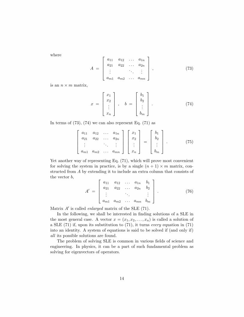
where

A =

a11 a12 . . . a1n

a21 a22 . . . a2n...

. . ....

am1 am2 . . . amn

, (73)

is an n×m matrix,

x =

x1

x2...

xn

, b =

b1

b2...

bm

. (74)

In terms of (73), (74) we can also represent Eq. (71) as

a11 a12 . . . a1n

a21 a22 . . . a2n...

. . ....

am1 am2 . . . amn

x1

x2...

xn

=

b1

b2...

bm

. (75)

Yet another way of representing Eq. (71), which will prove most convenientfor solving the system in practice, is by a single (n + 1) ×m matrix, con-structed from A by extending it to include an extra column that consists ofthe vector b,

A′ =

a11 a12 . . . a1n b1

a21 a22 . . . a2n b2...

. . ....

am1 am2 . . . amn bm

. (76)

Matrix A′ is called enlarged matrix of the SLE (71).In the following, we shall be interested in finding solutions of a SLE in

the most general case. A vector x = (x1, x2, . . . , xn) is called a solution ofa SLE (71) if, upon its substitution to (71), it turns every equation in (71)into an identity. A system of equations is said to be solved if (and only if)all its possible solutions are found.

The problem of solving SLE is common in various fields of science andengineering. In physics, it can be a part of such fundamental problem assolving for eigenvectors of operators.

14

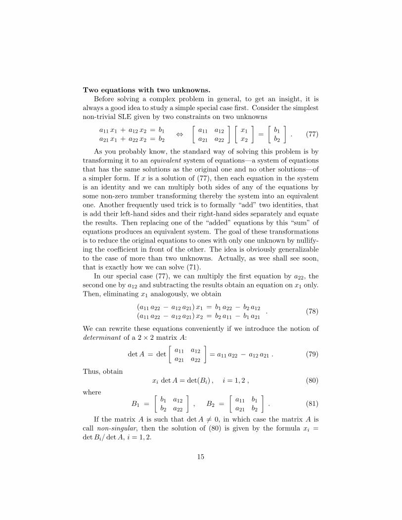
Two equations with two unknowns.Before solving a complex problem in general, to get an insight, it is

always a good idea to study a simple special case first. Consider the simplestnon-trivial SLE given by two constraints on two unknowns

a11 x1 + a12 x2 = b1

a21 x1 + a22 x2 = b2⇔

[a11 a12

a21 a22

] [x1

x2

]=

[b1

b2

]. (77)

As you probably know, the standard way of solving this problem is bytransforming it to an equivalent system of equations—a system of equationsthat has the same solutions as the original one and no other solutions—ofa simpler form. If x is a solution of (77), then each equation in the systemis an identity and we can multiply both sides of any of the equations bysome non-zero number transforming thereby the system into an equivalentone. Another frequently used trick is to formally “add” two identities, thatis add their left-hand sides and their right-hand sides separately and equatethe results. Then replacing one of the “added” equations by this “sum” ofequations produces an equivalent system. The goal of these transformationsis to reduce the original equations to ones with only one unknown by nullify-ing the coefficient in front of the other. The idea is obviously generalizableto the case of more than two unknowns. Actually, as wee shall see soon,that is exactly how we can solve (71).

In our special case (77), we can multiply the first equation by a22, thesecond one by a12 and subtracting the results obtain an equation on x1 only.Then, eliminating x1 analogously, we obtain

(a11 a22 − a12 a21) x1 = b1 a22 − b2 a12

(a11 a22 − a12 a21) x2 = b2 a11 − b1 a21. (78)

We can rewrite these equations conveniently if we introduce the notion ofdeterminant of a 2× 2 matrix A:

detA = det[

a11 a12

a21 a22

]= a11 a22 − a12 a21 . (79)

Thus, obtainxi det A = det(Bi) , i = 1, 2 , (80)

where

B1 =[

b1 a12

b2 a22

], B2 =

[a11 b1

a21 b2

]. (81)

If the matrix A is such that detA 6= 0, in which case the matrix A iscall non-singular, then the solution of (80) is given by the formula xi =det Bi/det A, i = 1, 2.

15

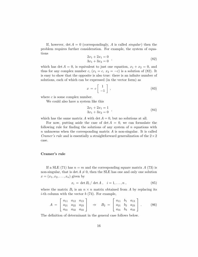
If, however, detA = 0 (correspondingly, A is called singular) then theproblem requires further consideration. For example, the system of equa-tions

2x1 + 2x1 = 03x1 + 3x2 = 0

, (82)

which has detA = 0, is equivalent to just one equation, x1 + x2 = 0, andthus for any complex number c, (x1 = c, x2 = −c) is a solution of (82). Itis easy to show that the opposite is also true: there is an infinite number ofsolutions, each of which can be expressed (in the vector form) as

x = c

[1−1

], (83)

where c is some complex number.We could also have a system like this

2x1 + 2x1 = 13x1 + 3x2 = 0

, (84)

which has the same matrix A with detA = 0, but no solutions at all.For now, putting aside the case of detA = 0, we can formulate the

following rule for finding the solutions of any system of n equations withn unknowns when the corresponding matrix A is non-singular. It is calledCramer’s rule and is essentially a straightforward generalization of the 2×2case.

Cramer’s rule

If a SLE (71) has n = m and the corresponding square matrix A (73) isnon-singular, that is detA 6= 0, then the SLE has one and only one solutionx = (x1, x2, . . . , xn) given by

xi = det Bi / detA , i = 1, . . . , n , (85)

where the matrix Bi is an n × n matrix obtained from A by replacing itsi-th column with the vector b (74). For example,

A =

a11 a12 a13

a21 a22 a23

a31 a32 a33

⇒ B2 =

a11 b1 a13

a21 b2 a23

a31 b3 a33

. (86)

The definition of determinant in the general case follows below.

16

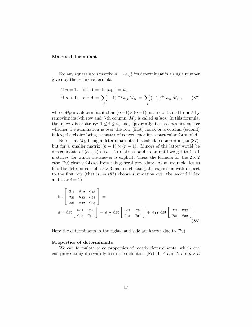
Matrix determinant

For any square n×n matrix A = {aij} its determinant is a single numbergiven by the recursive formula

if n = 1 , detA = det[a11] = a11 ,

if n > 1 , detA =∑

j

(−1)i+j aij Mij =∑

j

(−1)j+i aji Mji , (87)

where Mij is a determinant of an (n−1)×(n−1) matrix obtained from A byremoving its i-th row and j-th column, Mij is called minor. In this formula,the index i is arbitrary: 1 ≤ i ≤ n, and, apparently, it also does not matterwhether the summation is over the row (first) index or a column (second)index, the choice being a matter of convenience for a particular form of A.

Note that Mij being a determinant itself is calculated according to (87),but for a smaller matrix (n − 1) × (n − 1). Minors of the latter would bedeterminants of (n − 2) × (n − 2) matrices and so on until we get to 1 × 1matrices, for which the answer is explicit. Thus, the formula for the 2 × 2case (79) clearly follows from this general procedure. As an example, let usfind the determinant of a 3× 3 matrix, choosing the expansion with respectto the first row (that is, in (87) choose summation over the second indexand take i = 1)

det

a11 a12 a13

a21 a22 a23

a31 a32 a33

=

a11 det[

a22 a23

a32 a33

]− a12 det

[a21 a23

a31 a33

]+ a13 det

[a21 a22

a31 a32

].

(88)

Here the determinants in the right-hand side are known due to (79).

Properties of determinantsWe can formulate some properties of matrix determinants, which one

can prove straightforwardly from the definition (87). If A and B are n× n

17

matrices and λ is a complex number, then

det(AT) = detA , (89)

det(A†) = det((A∗)T

)= (detA)∗ , (90)

det(λA) = λn det A , (91)det(AB) = detA det B . (92)

A very important set of determinant properties involves the followingclass of operations with matrices.

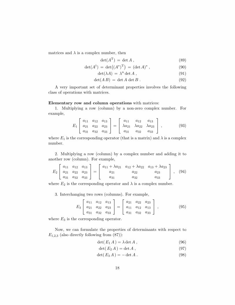
Elementary row and column operations with matrices:1. Multiplying a row (column) by a non-zero complex number. For

example,

E1

a11 a12 a13

a21 a22 a23

a31 a32 a33

=

a11 a12 a13

λa21 λa22 λa23

a31 a32 a33

, (93)

where E1 is the corresponding operator (that is a matrix) and λ is a complexnumber.

2. Multiplying a row (column) by a complex number and adding it toanother row (column). For example,

E2

a11 a12 a13

a21 a22 a23

a31 a32 a33

=

a11 + λa21 a12 + λa22 a13 + λa23

a21 a22 a23

a31 a32 a33

, (94)

where E2 is the corresponding operator and λ is a complex number.

3. Interchanging two rows (columns). For example,

E3

a11 a12 a13

a21 a22 a23

a31 a32 a33

=

a21 a22 a23

a11 a12 a13

a31 a32 a33

, (95)

where E3 is the corresponding operator.

Now, we can formulate the properties of determinants with respect toE1,2,3 (also directly following from (87)):

det(E1 A ) = λdet A , (96)det(E2 A ) = detA , (97)

det(E3 A ) = −det A . (98)

18

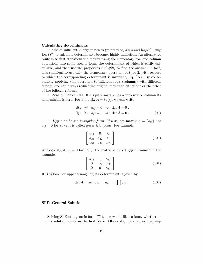
Calculating determinantsIn case of sufficiently large matrices (in practice, 4× 4 and larger) using

Eq. (87) to calculate determinants becomes highly inefficient. An alternativeroute is to first transform the matrix using the elementary row and columnoperations into some special form, the determinant of which is easily cal-culable, and then use the properties (96)-(98) to find the answer. In fact,it is sufficient to use only the elementary operation of type 2, with respectto which the corresponding determinant is invariant, Eq. (97). By conse-quently applying this operation to different rows (columns) with differentfactors, one can always reduce the original matrix to either one or the otherof the following forms:

1. Zero row or column. If a square matrix has a zero row or column itsdeterminant is zero. For a matrix A = {aij}, we can write

∃i : ∀j, aij = 0 ⇒ det A = 0 ,

∃j : ∀i, aij = 0 ⇒ detA = 0 . (99)

2. Upper or Lower triangular form. If a square matrix A = {aij} hasaij = 0 for j > i it is called lower triangular. For example,

a11 0 0a21 a22 0a31 a32 a33

. (100)

Analogously, if aij = 0 for i > j, the matrix is called upper triangular. Forexample,

a11 a12 a13

0 a22 a23

0 0 a33

. (101)

If A is lower or upper triangular, its determinant is given by

detA = a11 a22 . . . ann =∏

i

aii . (102)

SLE: General Solution

Solving SLE of a generic form (71), one would like to know whether ornot its solution exists in the first place. Obviously, the analysis involving

19

determinant of A is irrelevant in the general case, since we don’t restrictourselves with m = n anymore. However, one can introduce a generalcharacteristic of matrices that allows to infer important information abouttheir structure and thus about the corresponding SLE. First, let us define asubmatrix.

A submatrix of a matrix A is a matrix that can be formed from theelements of A by removing one, or more than one, row or column. Wealready used submartices implicity in the definition of minors.

The key notion in the analysis of SLE is rank of a matrix, defined asfollows: an integer number r is rank of a matrix A if A has an r × r (rrows and r columns) submatrix Sr such that detSr 6= 0, and any r1 × r1

submatrix Sr1 , r1 > r, either does not exist or detSr1 = 0. We shall writerankA = r. Note that, if A is an m × n matrix, then rankA can not begreater than the smaller number among m and n. In some cases, it is moreconvenient to use an equivalent definition: rankA is the maximum numberof linearly independent rows (columns) in A.

To prove equivalence of the two definitions, recall the method of cal-culating determinants using the elementary row and column operations. Ifdet Sr 6= 0, transforming Sr by multiplying any its row by a number andadding it to another row we can not nullify any row in Sr completely (oth-erwise, that would immediately give detSr = 0). In other words, none ofthe rows in Sr can be reduced to a linear combination of other rows, andthus there are r linearly independent rows in Sr. But Sr is a submatrix ofA, therefore there are at least r linearly independent rows in A. On theother hand, there is no more than r linearly independent rows in A. In-deed, detSr1 = 0 implies that rows of Sr1 must be linearly dependent andthus any set of r1 > r rows in A is linear dependent, which means that ris the maximum number of linearly independent rows. Vice versa: if r isthe maximum number of linearly independent rows in A, then composing asubmatrix Sr of size r × r consisting of these rows gives detSr 6= 0. Sinceany r1 > r rows are linearly dependent, for any r1 × r1 submatrix Sr1 , weget detSr1 = 0. Analogously, one proves that r is the number of linearlyindependent columns.

Thereby, we proved an interesting fact: in any matrix, the maximumnumber of linearly independent rows is equal to the maximum number of lin-early independent columns. There is also an important property of rankA,that follows directly from its definition in the second form. That is rankAis invariant with respect to elementary row and column operations appliedto A.

Now, we can formulate the following criterion.

20

Theorem (Kronecker-Capelli). A SLE (71) has at least one solution ifand only if rank of the matrix A (73) is equal to the rank of the enlargedmatrix A′ (76).

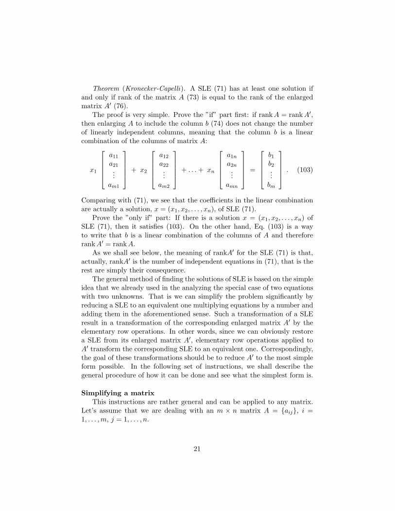
The proof is very simple. Prove the ”if” part first: if rankA = rank A′,then enlarging A to include the column b (74) does not change the numberof linearly independent columns, meaning that the column b is a linearcombination of the columns of matrix A:

x1

a11

a21...

am1

+ x2

a12

a22...

am2

+ . . . + xn

a1n

a2n...

amn

=

b1

b2...

bm

. (103)

Comparing with (71), we see that the coefficients in the linear combinationare actually a solution, x = (x1, x2, . . . , xn), of SLE (71).

Prove the ”only if” part: If there is a solution x = (x1, x2, . . . , xn) ofSLE (71), then it satisfies (103). On the other hand, Eq. (103) is a wayto write that b is a linear combination of the columns of A and thereforerankA′ = rankA.

As we shall see below, the meaning of rankA′ for the SLE (71) is that,actually, rankA′ is the number of independent equations in (71), that is therest are simply their consequence.

The general method of finding the solutions of SLE is based on the simpleidea that we already used in the analyzing the special case of two equationswith two unknowns. That is we can simplify the problem significantly byreducing a SLE to an equivalent one multiplying equations by a number andadding them in the aforementioned sense. Such a transformation of a SLEresult in a transformation of the corresponding enlarged matrix A′ by theelementary row operations. In other words, since we can obviously restorea SLE from its enlarged matrix A′, elementary row operations applied toA′ transform the corresponding SLE to an equivalent one. Correspondingly,the goal of these transformations should be to reduce A′ to the most simpleform possible. In the following set of instructions, we shall describe thegeneral procedure of how it can be done and see what the simplest form is.

Simplifying a matrixThis instructions are rather general and can be applied to any matrix.

Let’s assume that we are dealing with an m × n matrix A = {aij}, i =1, . . . ,m, j = 1, . . . , n.

21

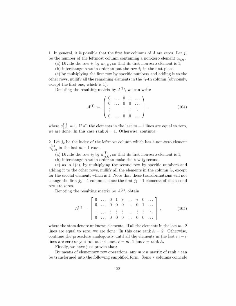
1. In general, it is possible that the first few columns of A are zeros. Let j1

be the number of the leftmost column containing a non-zero element ai1j1 .(a) Divide the row i1 by ai1 j1 , so that its first non-zero element is 1,(b) interchange rows in order to put the row i1 in the first place,(c) by multiplying the first row by specific numbers and adding it to the

other rows, nullify all the remaining elements in the j1-th column (obviously,except the first one, which is 1).

Denoting the resulting matrix by A(1), we can write

A(1) =

0 . . . 0 1 . . .0 . . . 0 0 . . ....

......

. . .0 . . . 0 0 . . .

, (104)

where a(1)1 j1

= 1. If all the elements in the last m− 1 lines are equal to zero,we are done. In this case rankA = 1. Otherwise, continue.

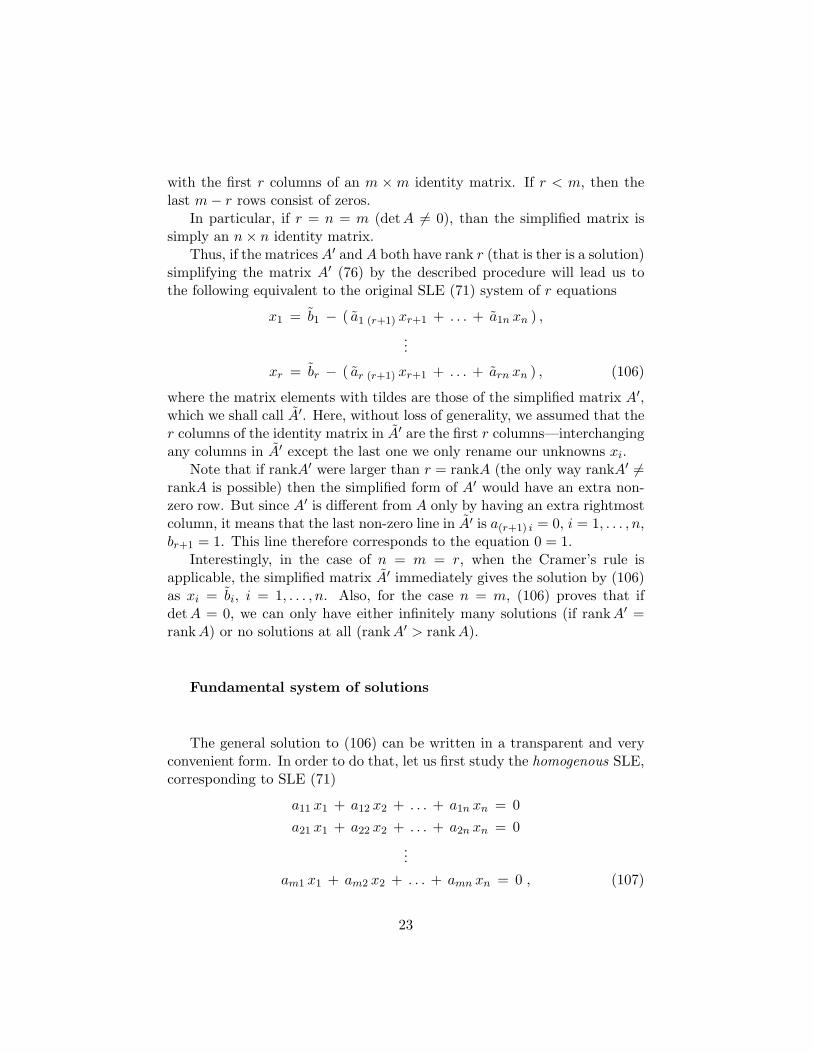
2. Let j2 be the index of the leftmost column which has a non-zero elementa

(1)i2 j2

in the last m− 1 rows.

(a) Divide the row i2 by a(1)i2 j2

, so that its first non-zero element is 1,(b) interchange rows in order to make the row i2 second(c) as in 1(c), by multiplying the second row by specific numbers and

adding it to the other rows, nullify all the elements in the column i2, exceptfor the second element, which is 1. Note that these transformations will notchange the first j2 − 1 columns, since the first j2 − 1 elements of the secondrow are zeros.

Denoting the resulting matrix by A(2), obtain

A(1) =

0 . . . 0 1 ∗ . . . ∗ 0 . . .0 . . . 0 0 0 . . . 0 1 . . .... . . .

......

... . . ....

.... . .

0 . . . 0 0 0 . . . 0 0 . . .

, (105)

where the stars denote unknown elements. If all the elements in the last m−2lines are equal to zero, we are done. In this case rankA = 2. Otherwise,continue the procedure analogously until all the elements in the last m− rlines are zero or you run out of lines, r = m. Thus r = rankA.

Finally, we have just proven that:By means of elementary row operations, any m×n matrix of rank r can

be transformed into the following simplified form. Some r columns coincide

22

with the first r columns of an m ×m identity matrix. If r < m, then thelast m− r rows consist of zeros.

In particular, if r = n = m (detA 6= 0), than the simplified matrix issimply an n× n identity matrix.

Thus, if the matrices A′ and A both have rank r (that is ther is a solution)simplifying the matrix A′ (76) by the described procedure will lead us tothe following equivalent to the original SLE (71) system of r equations

x1 = b1 − ( a1 (r+1) xr+1 + . . . + a1n xn ) ,

...

xr = br − ( ar (r+1) xr+1 + . . . + arn xn ) , (106)

where the matrix elements with tildes are those of the simplified matrix A′,which we shall call A′. Here, without loss of generality, we assumed that ther columns of the identity matrix in A′ are the first r columns—interchangingany columns in A′ except the last one we only rename our unknowns xi.

Note that if rankA′ were larger than r = rankA (the only way rankA′ 6=rankA is possible) then the simplified form of A′ would have an extra non-zero row. But since A′ is different from A only by having an extra rightmostcolumn, it means that the last non-zero line in A′ is a(r+1) i = 0, i = 1, . . . , n,br+1 = 1. This line therefore corresponds to the equation 0 = 1.

Interestingly, in the case of n = m = r, when the Cramer’s rule isapplicable, the simplified matrix A′ immediately gives the solution by (106)as xi = bi, i = 1, . . . , n. Also, for the case n = m, (106) proves that ifdet A = 0, we can only have either infinitely many solutions (if rankA′ =rankA) or no solutions at all (rankA′ > rankA).

Fundamental system of solutions

The general solution to (106) can be written in a transparent and veryconvenient form. In order to do that, let us first study the homogenous SLE,corresponding to SLE (71)

a11 x1 + a12 x2 + . . . + a1n xn = 0a21 x1 + a22 x2 + . . . + a2n xn = 0

...am1 x1 + am2 x2 + . . . + amn xn = 0 , (107)

23

or, equivalently,Ax = 0 , (108)

where A is given by (73). Simplifying the matrix A, Eqs. (107) are reducedto an equivalent system of r = rankA equations

x1 = − ( a1 (r+1) xr+1 + . . . + a1n xn ) ,

...xr = − ( ar (r+1) xr+1 + . . . + arn xn ) . (109)

The importance of the homogenous SLE is due to the following theorem.Theorem. Let the vector y0 be the solution of SLE (71), then vector y

is also a solution of (71) if and only if there exists a solution of the corre-sponding homogeneous SLE (71) x, such that y = y0 + x.

The proof is obvious: if Ay0 = b and Ay = b, then A(y − y0) = 0, thusy − y0 = x is a solution of the homogeneous system; vice versa: if Ay0 = 0and Ax = 0, then, for y = y0 + x, we get Ay0 = b.

Most importantly, the theorem implies that a general solution of SLE(71) is a sum of some particular solution of (71) and a general solution of thehomogeneous SLE (107). A particular solution of (71) y0 = (y0

1, . . . , y0n) can

be obtained, for example, by setting all the variables in the right hand sideof (106) to zero and calculating the rest from the same system of equations:

y0 =

b1...br

0...0

. (110)

Now, to obtain the general solution of SLE (71), it is sufficient solve asimpler system of equations (107). First note that unlike the inhomogeneousSLE (71) this system always has a trivial solution x = 0.

A general solution of homogeneous SLE (107) can be expressed in termsof the so-called fundamental system of solutions (FSS), which is simply aset of n − r linearly independent vectors satisfying (107) (or, equivalently,(109)):

Theorem. Suppose x1 = (x11, . . . , x

1n) , . . . , xn−r = (xn−r

1 , . . . , xn−rn )

is some FSS of the homogeneous SLE (107). Then, any solution of the

24

homogeneous SLE (107) x is a linear combination of the FSS,

x =n−r∑

i=1

cixi , (111)

where ci are some complex numbers.The proof. Compose a matrix X, the columns of which are the solutions

x, x1, . . . , xn−r. This matrix has at least n− r linearly independent columnsand thus its rank is not smaller than n − r. On the other hand, rankXcan not be larger than n− r. Indeed, each of the rows of X satisfies (109),that is the first r rows are linear combinations of the last n− r rows. Thus,rankX = n−r and therefore x must be a linear combination of x1, . . . , xn−r.

To prove existence of a FSS, we can obtain it explicitly by the followingprocedure. To obtain the first vector, x1, we can set in the right hand sideof (109) x1

r+1 = 1, and x1i = 0, i = r +2, . . . , n and solve for the components

in the left hand side, which gives x1 = (−a1 (r+1), . . . ,−ar (r+1),1, 0 . . . , 0). Then, chose x2

r+2 = 1, x2i = 0, i = r + 1, r + 3, . . . , n and solve

for the remaining components of x2. Repeating this procedure analogouslyfor the remaining variables in the right hand side of (109) leads to a set ofvectors in the form

x1 =

−a1 (r+1)...

−ar (r+1)

10...0

, x2 =

−a1 (r+2)...

−ar (r+2)

01...0

, . . . , xn−r =

−a1 n...

−ar n

0...01

.

(112)By construction the vectors in () are linearly independent and satisfy (107).Therefore the vectors () form a FSS. Obviously, the FSS is not unique. Inthe form of (), with zeros and ones in the last n − r components of xi, theFSS is called the normal FSS.

To summarize, the general solution of a SLE (71) is given by

y = y0 +n−r∑

i=1

cixi , (113)

where r = rank A = rankA′, y0 is some particular solution of SLE (71),{xi}, i = i, . . . , n− r is some FSS of the homogeneous SLE (107) and ci are

25

complex numbers. In practice, we shall typically use the normal FSS, forwhich the latter formula becomes (taking into account (110) and ())

y =

b1...br

00...0

+ c1

−a1 (r+1)...

−ar (r+1)

10...0

+ c2

−a1 (r+2)...

−ar (r+2)

01...0

+ . . . + cn−r

−a1 n...

−ar n

0...01

.

(114)

Inverse Matrix

Given some operator A, we naturally define an inverse to it operator A−1

by the requirementsA−1A = AA−1 = I . (115)

This definition implies that if A−1 is inverse to A, then A is inverse to A−1.[Note, in particular, that for any unitary operator U we have U−1 ≡ U †.] Itis important to realize that the inverse operator not always exists. Indeed,the existence of A−1 implies that the mapping

|x〉 → |y〉 , (116)

where|y〉 = A|x〉 , (117)

is a one-to-one mapping, since only in this case we can unambiguously restore|x〉 from |y〉. For example, the projector P|a〉 = |a〉〈a| does not have aninverse operator in the spaces of dimensionality larger than one.

If the linear operator A is represented by the matrix A, the natural ques-tion is: What matrix corresponds to the inverse operator A−1?—Such matrixis called inverse matrix. Also important is the question of the criterion ofexistence of the inverse matrix (in terms of the given matrix A).

The previously introduced notions of the determinant and minors turnout to be central to the theory of the inverse matrix. Given a matrix A,

26

define the matrix B:bij = (−1)i+jMji , (118)

where M ’s are corresponding minors of the matrix A. Considering the prod-uct AB, we get

(AB)ij =∑

s

aisbsj =∑

s

ais(−1)s+jMjs ={

det A , if i = j ,0 , if i 6= j .

(119)Indeed, in the case i = j we explicitly deal with Eq. (87). The case i 6= j isalso quite simple. We notice that here we are dealing with the determinantof a new matrix A obtained from A by replacing the j-th row with the i-throw, in which case the matrix A has two identical rows and its determinantis thus zero. Rewriting Eq. (119) in the matrix form we get

AB = [detA] I . (120)

Analogously, we can getBA = [detA] I , (121)

and this leads us to the conclusion that

A−1 = [detA]−1B , (122)

provided detA 6= 0. The latter requirement thus forms the necessary andsufficient condition of the existence of the inverse matrix.

The explicit form for the inverse matrix, Eqs. (122), (118), readily leadsto the Cramer’s rule (85). Indeed, given the linear system of equations

A~x = ~b , (123)

with A being n× n matrix with non-zero determinant, we can act on bothsides of the equation with the operator A−1 and get

~x = A−1~b = [detA]−1B~b . (124)

Then we note that the i-th component of the vector B~b is nothing but thedeterminant of the matrix Bi obtained from A by replacing its i-th columnwith the vector ~b.

27

Eigenvector/Eigenvalue Problem

Matrix form of Quantum Mechanics. To reveal the crucial importance ofthe eigenvector/eigenvalue problem for physics applications, we start withthe matrix formulation of Quantum Mechanics. At the mathematical level,this amounts to considering the Schrodinger’s equation

i~d

dt|ψ〉 = H|ψ〉 (125)

[where |ψ〉 is a vector of a certain Hilbert space, H is a Hermitian operator(called Hamiltonian), and ~ is the Plank’s constant] in the representationwhere |ψ〉 is specified by its coordinates in a certain ONB (we loosely usehere the sign of equality),

|ψ〉 = (ψ1, ψ2, ψ3, . . .) , (126)

and the operator H is represented by its matrix elements Hjs with respectto this ONB. In the matrix form, Eq. (125) reads

i~ψj =∑

s

Hjs ψs . (127)

Suppose we know all the eigenvectors {|φ(n)〉} of the operator H (with cor-responding eigenvalues {En}):

H|φ(n)〉 = En|φ(n)〉 . (128)

Since the operator H is Hermitian, without loss of generality we can assumethat {|φ(n)〉} is an ONB, so that we can look for the solution of Eq. (125)in the form

|ψ〉 =∑

n

Cn(t)|φ(n)〉 . (129)

Plugging this into (125) yields

i~Cn = EnCn ⇒ Cn(t) = Cn(0)e−iEnt/~ . (130)

The initial values of the coefficients C are given by

Cn(0) = 〈φ(n)|ψ(t = 0)〉 =∑

s

(φ(n)s )∗ψs(t = 0) , (131)

28

where φ(n)s is the s-th component of the vector |φ(n)〉. In components, our

solution readsψj(t) =

∑n

Cn(0)φ(n)j e−iEnt/~ . (132)

We see that if we know En’s and φ(n)j ’s, we can immediately solve the

Schrodingers’s equation. And to find En’s and φ(n)s ’s we need to solve the

problem ∑s

Hjsφs = Eφj , (133)

which is the eigenvalue/eigenvector problem for the matrix H.

In the standard mathematical notation, the eigenvalue/eigenvector prob-lem for a matrix A reads

Ax = λx , (134)

where the eigenvector x is supposed to be found simultaneously with corre-sponding eigenvalue λ. Introducing the matrix

A = A− λI , (135)

we see that formally the problem looks like the system of linear homogeneousequations:

Ax = 0 . (136)

However, the matrix elements of the matrix A depend on the yet unknownparameter λ. Now we recall that from the theory of the inverse matrix itfollows that if det A 6= 0, then x = A−1 0 = 0, and there is no non-trivialsolutions for the eigenvector. We thus arrive at

det A = 0 (137)

as the necessary condition for having non-trivial solution for the eigenvectorof the matrix A. This condition is also a sufficient one. It guarantees theexistence of at least one non-trivial solution for corresponding λ. The equa-tion (137) is called characteristic equation. It defines the set of eigenvalues.With the eigenvalues found from (137), one then solves the system (136) forcorresponding eigenvectors.

If A is a n×n matrix, then the determinant of the matrix A is a polyno-mial function of the parameter λ, the degree of the polynomial being equalto n:

det A = a0 + a1λ1 + a2λ

2 + . . . + anλn = Pn(λ) , (138)

29

where a0, a1, . . . , an are the coefficients depending on the matrix elementsof the matrix A. The polynomial Pn(λ) is called characteristic polynomial.The algebraic structure of the characteristic equation for an n×n matrix isthus

Pn(λ) = 0 . (139)

In this connection, it is important to know that for any polynomial of degreen the Fundamental Theorem of Algebra guarantees the existence of exactly ncomplex roots (if repeated roots are counted up to their multiplicity). For aHermitian matrix, all the roots of the characteristic polynomial will be real,in agreement with the theorem which we proved earlier for the eigenvaluesof Hermitian operators.

Problem 31. Find the eigenvalues and eigenvectors for all the three Pauli matrices(see Problem 26).

Problem 32. Solve the (non-dimensionalized) Schrodinger’s equation for the wavefunction |ψ〉 = (ψ1, ψ2),

iψj =2∑

s=1

Hjsψs (j = 1, 2) , (140)

with the matrix H given by

H =[

0 ξξ 0

], (141)

and the initial condition being

ψ1(t = 0) = 1 , ψ2(t = 0) = 0 . (142)

Functions of Operators

The operations of addition and multiplication (including multiplication by anumber) allow one to introduce functions of operators/matrices by utilizingthe idea of a series. [Recall that we have already used this idea to introduce

30

the functions of a complex variable.] For example, given an operator A wecan introduce the operator eA by

eA =∞∑

n=0

1n!

An . (143)

The exponential function plays a crucial role in Quantum Mechanics. Namely,a formal solution to the Schrodinger’s equation (125) can be written as

|ψ(t)〉 = e−iHt/~|ψ(0)〉 . (144)

The equivalence of (144) to the original equation (125) is checked by explicitdifferentiating (144) with respect to time:

i~d

dt|ψ(t)〉 = i~

[d

dte−iHt/~

]|ψ(0)〉 = i~

[−iH

~e−iHt/~

]|ψ(0)〉 =

= H e−iHt/~|ψ(0)〉 = H|ψ(t)〉 . (145)

Note that in a general case differentiating a function of an operator withrespect to a parameter the operator depends on is non-trivial because ofnon-commutativity of the product of operators. Here this problem does notarise since we differentiate with respect to a parameter which enters theexpressions as a pre-factor, so that the operator H behaves like a number.

The exponential operator in (144) is called evolution operator. It “evolves”the initial state into the state at a given time moment.

In a general case, the explicit calculation of the evolution operator isnot easier than solving the Schrodinger equation. That is why we refer toEq. (144) as formal solution. Nevertheless, there are cases when the evalu-ation is quite straightforward. As a typical and quite important example,consider the case when H is proportional to one of the three Pauli matrices(see Problem 26). In this case,

e−iHt/~ = e−iµσt , (146)

where σ stands for one of the three Pauli matrices and µ is a constant.The crucial property of Pauli matrices that allows us to do the algebrais σ2 = I. It immediately generalizes to σ2m = I and σ2m+1 = σ,where m = 0, 1, 2, . . .. With these properties taken into account we obtain

31

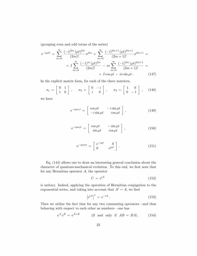
(grouping even and odd terms of the series)

e−iµσt =∞∑

m=0

(−i)2m (µt)2m

(2m)!σ2m +

∞∑

m=0

(−i)2m+1 (µt)2m+1

(2m + 1)!σ2m+1 =

= I∞∑

m=0

(−1)m (µt)2m

(2m)!− iσ

∞∑

m=0

(−1)2m (µt)2m+1

(2m + 1)!=

= I cosµt − iσ sinµt . (147)

In the explicit matrix form, for each of the three matrices,

σ1 =[

0 11 0

], σ2 =

[0 − ii 0

], σ3 =

[1 00 − 1

], (148)

we have

e−iµσ1t =[

cosµt − i sinµt−i sinµt cosµt

], (149)

e−iµσ2t =[

cosµt − sinµtsinµt cosµt

], (150)

e−iµσ3t =[

e−iµt 00 eiµt

]. (151)

Eq. (144) allows one to draw an interesting general conclusion about thecharacter of quantum-mechanical evolution. To this end, we first note thatfor any Hermitian operator A, the operator

U = eiA (152)

is unitary. Indeed, applying the operation of Hermitian conjugation to theexponential series, and taking into account that A† = A, we find

[eiA

]†= e−iA . (153)

Then we utilize the fact that for any two commuting operators—and thusbehaving with respect to each other as numbers—one has

eA eB = eA+B (if and only if AB = BA) . (154)

32

This yields (below O is the matrix of zeroes)

eiA e−iA = eO = I , (155)

and proves that UU † = I. We thus see that the evolution operator is uni-tary. This means that the evolution in Quantum Mechanics is equivalent toa certain rotation in the Hilbert space of states.

Systems of Linear Ordinary Differential Equationswith Constant Coefficients

The theory of matrix allows us to develop a simple general scheme forsolving systems of ordinary differential equations with constant coefficients.

We start with the observation that without loss of generality we candeal only with the first-order derivatives, since higher-order derivatives canbe reduced to the first-order one at the expense of introducing new unknownfunctions equal to corresponding derivatives. Let us illustrate this idea withthe differential equation of the harmonic oscillator:

x + ω2x = 0 . (156)

The equation is the second-order differential equation, and there is only oneunknown function, x(t). Now if we introduce two functions, x1 ≡ x, andx2 ≡ x, we can equivalently rewrite (156) as the system of two equations(for which we use the matrix form)

[x1

x2

]=

[0 1−ω2

0 0

] [x1

x2

]. (157)

Analogously, any system of ordinary differential equations with constantcoefficients can be reduced to the canonical vector form

x = Ax , (158)

where x = (x1, x2 . . . xm) is the vector the components of which correspondto the unknown functions (of the variable t), and A is an m×m matrix. Inaddition to the equation (158), the initial condition x(t = 0) is supposed tobe given.

33

In a general case, the matrix A has m different eigenvectors with corre-sponding eigenvalues :

Au(n) = λnu(n) (n = 1, 2, 3, . . . ,m) . (159)

As can be checked by direct substitution, each eigenvector/eigenvalue yieldsan elementary solution of Eq. (158) of the form

s(n)(t) = cn eλnt u(n) , (160)

where cn is an arbitrary constant. The linearity of the equations allows usto write the general solution as just the sum of elementary solutions.

x(t) =m∑

n=1

cn eλnt u(n) . (161)

In components, this reads

xj(t) =m∑

n=1

cn eλnt u(n)j (j = 1, 2, 3, . . . , m) . (162)

To fix the constants cn, we have to use the initial condition. In the spe-cial case of so-called normal matrix (see also below), featuring an ONB ofeigenvectors, finding the constants cn is especially simple. As we have seenit many times in this course, it reduces to just forming the inner products:

cn =m∑

j=1

[u(n)j ]∗xj(0) (if u′s form an ONB) . (163)

In a general case, we have to solve the system of linear equations

m∑

n=1

u(n)j cn = xj(0) (j = 1, 2, 3, . . . , m) , (164)

in which u(n)j ’s play the role of the matrix, cn’s play the role of the compo-

nents of the vector of unknowns, and x(0) plays the role of the r.h.s. vector.

Problem 33. Solve the system of two differential equations{

3x1 = −4x1 + x2

3x2 = 2x1 − 5x2(165)

34

for the two unknown functions, x1(t) and x2(t), with the initial conditions

x1(0) = 2 , x2(0) = −1 . (166)

Normal Matrices/Operators

By definition, a normal matrix—for the sake of briefness, we are talking ofmatrices, keeping in mind that a linear operator can be represented by amatrix—is the matrix that features an ONB of its eigenvectors. [For exam-ple, Hermitian and unitary matrices are normal.] A necessary and sufficientcriterion for a matrix to be normal is given by the following theorem. Thematrix A is normal if and only if

AA† = A†A , (167)

that is if A commutes with its Hermitian conjugate.Proof. Let us show that Eq. (167) holds true for each normal matrix. Inthe ONB of its eigenvectors, the matrix A is diagonal (all the non-diagonalelements are zeros), and so has to be the matrix A†, which then immediatelyimplies commutativity of the two matrices, since any two diagonal matricescommute.

To show that Eq. (167) implies the existence of an ONB of eigenvectors,we first prove an important lemma saying that any eigenvector of the matrixA with the eigenvalue λ is also an eigenvector of the matrix A† with theeigenvalue λ∗. Let x be an eigenvector of A:

Ax = λx . (168)

The same is conveniently written as

Ax = 0 , A = A− λI . (169)

Note that if AA† = A†A, then AA† = A†A, because

AA† = AA† − λA† − λ∗A + |λ|2 , (170)

A†A = A†A− λ∗A− λA† + |λ|2 = AA† . (171)

35

[Here we took into account that A† = A† − λ∗I.] Our next observation is

〈A†x|A†x〉 = 〈x|AA†|x〉 = 〈x|A†A|x〉 = 〈Ax|A|x〉 = 0 , (172)

implying the statement of the lemma:

|A†x〉 = 0 ⇔ A† x = λ∗x . (173)

With the above lemma, the rest of the proof is most simple to the that forthe Hermitian operator. Once again we care only about the orthogonality ofthe eigenvectors with different eigenvalues, since the eigenvectors of the sameeigenvalue form a subspace, so that if the dimensionality of this subspace isgreater than one, we just use the Gram-Schmidt orthogonalization withinthis subspace. Suppose we have

Ax1 = λ1 x1 , (174)

Ax2 = λ2 x2 . (175)

By our lemma, we haveA†x2 = λ∗2 x2 . (176)

From (174) we find〈x2|A|x1〉 = λ1〈x2|x1〉 , (177)

while (176) yields〈x1|A†|x2〉 = λ∗2〈x1|x2〉 . (178)

The latter equation can be re-written as

〈Ax1|x2〉 = λ∗2〈x1|x2〉 . (179)

Complex-conjugating both sides we get

〈x2|A|x1〉 = λ2〈x2|x1〉 . (180)

Comparing this with (177) we see that

λ1〈x2|x1〉 = λ2〈x2|x1〉 , (181)

which at λ1 6= λ2 is only possible if 〈x2|x1〉 = 0.

36