An Algorithm for Computing Jordan Chains and

Inverting Analytic Matrix Functions

Jon Wilkening ∗

May 6, 2007

Abstract

We present an efficient algorithm for obtaining a canonical system of Jor-dan chains for an n×n regular analytic matrix function A(λ) that is singularat the origin. For any analytic vector function b(λ), we show that each termin the Laurent expansion of A(λ)−1b(λ) may be obtained from the previousterms by solving an (n+d)× (n+d) linear system, where d is the order of thezero of det A(λ) at λ = 0. The matrix representing this linear system containsA(0) as a principal submatrix, which can be useful if A(0) is sparse. The lastseveral iterations can be eliminated if left Jordan chains are computed in ad-dition to right Jordan chains. The performance of the algorithm in floatingpoint and exact (rational) arithmetic is reported for several test cases. Themethod is shown to be forward stable in floating point arithmetic.

Key words. Matrix valued function, Jordan chain, Keldysh chain, analyticperturbation, matrix inversion, Laurent series

AMS subject classifications. 47A56, 47A46, 15A09, 41A58

1 Introduction

Analytic matrix functions arise frequently in mathematics. The most commonapplication [7, 10] involves solving the ordinary differential equation

Aldlx

dtl+ · · ·+ A0x = 0 (1.1)

using the ansatz x(t) = [ tk

k!x0 + · · ·+ txk−1 + xk]eλ0t, (x0 6= 0), which is a solutionif and only if

k∑m=0

tk−meλ0t

(k −m)!

m∑j=0

1j!

A(j)(λ0)xm−j

≡ 0, (1.2)

∗University of California, Berkeley, CA 94720 (wilken@math.berkeley.edu). The research ofthe author was supported in part by the Applied Mathematical Sciences subprogram of the Officeof Energy Research, U.S. Department of Energy, under Contract Number DE-AC03-76SF00098,and by the National Science Foundation through grant DMS-0101439.

2 J. WILKENING

where A(λ) = A0+· · ·+λlAl. Vectors x0, . . . , xk satisfying the bracketed expressionin (1.2) for m = 0, . . . , k are said to form a (right) Jordan chain of length k +1 forA(λ) at λ0. This condition is equivalent to requiring that the vector polynomial

x(λ) = x0 + (λ− λ0)x1 + · · ·+ (λ− λ0)kxk (1.3)

is a root function of A(λ) at λ0 of order k + 1, i.e. A(λ)x(λ) = O(λ− λ0)k+1.Analytic matrices also arise in contour integral representations of solutions of

various boundary value problems. For example, a solution of the Poisson equation∆u = 1 in the first quadrant with Dirichlet boundary conditions is given by theformula u(r, θ) = r2/4 + uS(r, θ), where

uS(r, θ) =∫

γrλF (λ, θ)A(λ)−1b(λ) dλ, (1.4)

γ is a contour surrounding λ0 = 2 in the complex plane, b(λ) =1

λ− 2

(−1/4

−1/4

),

F (λ, θ) =(cos λθ, sin λθ

λ

), and

A(λ) =(

1 0cos λπ

21λ sin λπ

2

), (1.5)

Note that at λ = 2, A(λ) is singular and b(λ) has a pole. The function uS(λ, θ)may be computed by expanding A(λ)−1b(λ) in a Laurent expansion and applyingthe residue theorem, which yields

uS(r, θ) = r2[(

θπ −

14

)cos 2θ + 1

π ln r sin 2θ]. (1.6)

Jordan chains for A(λ) are important in this problem because the root functionsdefined in (1.3) appear as poles of A(λ)−1b(λ), and may be used to recursivelycompute an arbitrary number of terms in the Laurent expansion; see Section 4.Singularities of general elliptic systems in the plane near corners and interfacejunctions have representations analogous to (1.4); see [4].

Other applications of analytic matrix functions include stochastic matrices andMarkov chains [11], linear vibrations [13], singular differential equations [3], dy-namical systems [16], and control theory [3, 7].

The local behavior of a matrix or operator A(λ) that depends analytically on λhas been studied extensively [2, 9, 12], especially in the case that A(λ) is a matrixpencil A0 + λA1 [7, 8, 14, 17] or a matrix polynomial A0 + · · · + λlAl [10, 15].Monic (Al = I) matrix polynomials are often reduced to the matrix pencil casevia a standard linearization procedure [7, 10]. However, for analytic matrices suchas (1.5) above, the expansion of A(λ) does not terminate, and any truncation mayhave a singular term Al of highest order; hence, an approach based on linearizationseems inappropriate in this context. Truncating the expansion and computing theSmith form [10] is also an option, but this is very expensive; see Section 4.2.

ANALYTIC MATRIX FUNCTIONS 3

In [1], Avrachenkov et. al. present an algorithm for expanding the inverse ofan analytic matrix function in a Laurent series. More specifically, they show howto reduce a system of matrix equations (involving n× n matrices) of the form

A0X0 = B0

. . .

A0Xs−1 + · · ·+ As−1X0 = Bs−1

(Ak, Bk givenXk unknown

)(1.7)

to another system of this form involving p × p matrices, where p = dim kerA0 isthe geometric multiplicity of the origin. Let d be its algebraic multiplicity. Ourapproach employs a different type of reduction based on adding d rows and columnsto A0 to construct an invertible matrix that can be used to recursively solve forsuccessive terms in the Laurent expansion of A(λ)−1. It also provides completeJordan chain information, which is often important in applications.

Canonical systems of Jordan chains depend discontinuously on the leadingcoefficients A0, . . . , As−1 of A(λ), where Ak = 1

k!A(k)(0) and s is the order of

the pole of A(λ)−1 at λ = 0. Nevertheless, there are many applications (e.g. inalgebraic geometry or partial differential equations) where these coefficients areknown exactly. In such cases our algorithm can be run using rational arithmeticto solve the problem analytically. In finite precision arithmetic, the method isforward stable when nullspaces are computed using a threshold on the smallestsingular values. The condition number depends on how close A(λ) is to an analyticmatrix function that is even more singular at the origin; see Appendix A.

Numerical stability is possible because we have specified the location of theeigenvalue of interest (e.g. the origin) as part of the problem statement. The eigen-value itself cannot be computed in floating point arithmetic (unless it is simple)as roundoff error is likely to split the eigenvalue like O(ε1/d), where ε is machineprecision and d is the algebraic multiplicity of the eigenvalue. Even using extraprecision, it is impossible to determine affirmatively that a tight cluster of eigenval-ues should exactly coalesce unless their multiplicities (or locations) are determinedalgebraically. The stability of this algorithm is useful in applications with a sim-ple, parasitic eigenvalue λ1 close to a known eigenvalue λ0. For example, integervalues of λ0 occur frequently in the corner singularities problem described above.By computing a canonical system of Jordan chains at λ0, we learn the algebraicmultiplicity of λ0 and can use this information to compute λ1 by a contour integraltechnique without corruption from λ0.

2 Canonical systems of root functions

In this section we establish notation and summarize the local spectral theory ofanalytic matrix functions; the presentation roughly follows [9].

Suppose A(λ) is an n × n matrix whose entries depend analytically on λ in aneighborhood of the origin. Suppose ∆(λ) := det A(λ) has a zero of order d ≥ 1 atthe origin. In particular, we assume that A(λ) is regular, i.e. ∆(λ) is not identically

4 J. WILKENING

zero. A vector polynomial

x(λ) = x0 + λx1 + · · ·+ λκ−1xκ−1, (xk ∈ Cn, κ ≥ 1) (2.1)

is called a root function of A(λ) of order κ at λ = 0 if

A(λ)x(λ) = O(λκ) and x0 6= 0. (2.2)

This is equivalent to requiring that (x0; . . . ;xκ−1) ∈ ker Aκ−1, where (x; y) =(xT , yT )T and the matrices Ak are defined via

Ak =

A0 0 · · · 0A1 A0 · · · 0· · · · · · · · · · · ·Ak Ak−1 · · · A0

, Aj =1j!

A(j)(0). (2.3)

Here we think of Cnκ as representing the space P/λκP, where P is the space of

formal power series in λ with coefficients in Cn and we identify two power serieswith the same leading terms x0 + λx1 + · · · + λκ−1xκ−1. In this representation,the action of A(λ) on such a power series becomes a matrix-vector multiplicationAκ−1 · (x0; . . . ;xκ−1).

The vectors xk in (2.1) are said to form a Jordan chain (or Keldysh chain) oflength κ. Several vector polynomials xj(λ) form a system of root functions if

xj(λ) = xj,0 + λxj,1 + · · ·+ λκj−1xj,κj−1, (1 ≤ j ≤ p) (2.4)A(λ)xj(λ) = O(λκj ), (2.5)the set {xj,0}p

j=1 is linearly independent in Cn. (2.6)

Such a system is said to be canonical if p = dim ker A0, x1(λ) is a root functionof maximal order κ1, and for j > 1, xj(λ) has maximal order κj among all rootfunctions x(λ) such that x(0) is linearly independent of x1(0), . . . , xj−1(0) in Cn.The resulting sequence of numbers κ1 ≥ · · · ≥ κp is uniquely determined by A(λ);see [9] and Section 3.

As a simple example, suppose A(λ) = A0 − λI. Then x0, . . . , xκ−1 form aJordan chain of length κ at λ = 0 iff x0 6= 0 and

A0x0 = 0, A0xk = xk−1 (1 ≤ k ≤ κ− 1) (2.7)

In this case x0, . . . , xκ−1 are linearly independent and can be extended to a basismatrix U = [x0, . . . , xn−1] that puts A in Jordan canonical form: U−1AU = J .(This requires knowing all the eigenvalues of A and finding a canonical system ofJordan chains at each). But in general the xk need not be linearly independent(some can even be zero) and it is more useful to reduce A to local Smith formA(λ) = C(λ)D(λ)E(λ)−1 as we now explain.

For any system of root functions xj(λ) (not necessarily canonical), we maychoose constant vectors xp+1, . . . , xn that extend x1(0), . . . , xp(0) to a basis for

ANALYTIC MATRIX FUNCTIONS 5

Cn. We call the system x1(λ), . . . , xp(λ), xp+1, . . . , xn an extended system of rootfunctions, and set κp+1 = · · · = κn = 0. Next we define the matrices

E(λ) =[x1(λ), . . . , xn(λ)

], (2.8)

D(λ) = diag(λκ1 , . . . , λκn), (2.9)

C(λ) = A(λ)E(λ)D(λ)−1. (2.10)

By (2.5), all singularities of C(λ) at the origin are removable. Since E(0) is invert-ible, det C(λ) has a zero of order d −

∑nj=1 κj at the origin, where d is the order

of the zero of ∆(λ) at the origin. The following theorem is proved in [9]:

Theorem 2.1 The following three conditions are equivalent:

(1) the columns xj(λ) of E(λ) form an extended canonical system of root func-tions for A(λ) at λ = 0 with orders κ1 ≥ · · · ≥ κn ≥ 0.

(2) C(0) is invertible.

(3)∑n

j=1 κj = d, where d is the algebraic multiplicity of λ = 0

Canonical systems of root functions are useful due to the fact that they com-pletely characterize the meromorphic behavior of A(λ)−1. Observe that

A(λ)−1 = E(λ)D(λ)−1C(λ)−1, (2.11)

where E(λ) and C(λ) are invertible at λ = 0. Thus for any holomorphic vectorfunction b(λ), all poles of A(λ)−1b(λ) at the origin are linear combinations of thefunctions λ−1−kxj(λ) with 1 ≤ j ≤ p and 0 ≤ k ≤ κj − 1. Moreover, each of thesefunctions actually occurs as a pole. For example, if we define bjk(λ) as the uniquevector polynomial of degree κ1 − 1 such that

bjk(λ) = λ−1−kA(λ)[xj,0 + · · ·+ λkxj,k] + O(λκ1), (2.12)

then

A(λ)−1bjk(λ) = λ−1−kxj(λ) + O(1), (1 ≤ j ≤ p, 0 ≤ k ≤ κj − 1). (2.13)

Other shifted and truncated versions of the residual A(λ)xj(λ) can also be usedfor bjk(λ), but the choice in (2.12) is relevant to Algorithm 4.6 below.

3 An algorithm for computing Jordan chains

In the previous section, we described the standard theoretical (as opposed to al-gorithmic) construction of canonical systems of root functions for A(λ) at λ = 0.This approach can be thought of as a depth-first approach: x1(λ) is chosen to beany root function of maximal order κ1, and the remaining root functions xj(λ) arechosen to be of maximal order κj such that xj(0) is linearly independent of thepreviously accepted vectors x0(0), . . . , xj−1(0).

6 J. WILKENING

Our algorithm uses a breadth-first approach. Instead of starting with a singleroot function of maximal order, we start with the space of all root functions oforder at least 1 (namely ker A0). We then use this space to find all root functionsof order at least 2, then 3, etc., until there are no root functions of higher order.At the kth stage of this process (starting at k = 0), we extract the Jordan chainsof length exactly k + 1, thereby obtaining a canonical system xj(λ) in reverse jorder (from p to 1).

In more detail, let us define the subspaces Wk and the canonical injectionsι : Cnk → Cn(k+1) via

Wk = ker Ak ⊂ Cn(k+1), ι(x0; . . . ;xk−1) = (0; x0; . . . ;xk−1). (3.1)

The block structure of the augmented matrices Ak defined in (2.3) implies thatι(Wk−1) ⊂ Wk for k ≥ 1. A Jordan chain of length k + 1 may be thought of as anon-zero element of the space

Wk = Wk

/ι(Wk−1), (3.2)

where we take ι(W−1) to mean {0} ⊂ Cn. Evidently, the projection π0 : Cn(k+1) →Cn given by

π0(x0; . . . ;xk) = x0 (3.3)

is injective from Wk to Cn, so several vectors in Wk are linearly independent ifftheir zeroth terms are linearly independent in Cn. To count Jordan chains, it isuseful to define

Rk = dim(Wk), rk = dim(Wk), k ≥ 0 (3.4)

so that Rk = rk + · · · + r0 and rk ≤ · · · ≤ r0. These last inequalities follow fromthe fact that the truncation operator τ : Cn(k+2) → Cn(k+1) given by

τ(x0; . . . ;xk+1) = (x0; . . . ;xk) (3.5)

injectively maps Wk+1 into Wk, i.e. shortening a Jordan chain gives another validJordan chain. Finally, to extract all Jordan chains of length k + 1, we choosevectors

xj,· = (xj,0; . . . ; xj,k) ∈ Wk, (j = rk+1 + 1, . . . , rk) (3.6)

such that the equivalence classes [xj,·] ∈ Wk are linearly independent and com-plement the subspace τ(Wk+1) ⊂ Wk consisting of truncations of longer chains.We also set κj = k + 1 for each j in (3.6). When rk+1 = rk, the range of indicesin (3.6) is empty and there are no partial multiplicities κj equal to k + 1. Thealgorithm terminates as soon as rk = 0, which happens when k = s := κ1, themaximal Jordan chain length. Since rk − rk+1 = #{j : κj = k + 1} and rs = 0, wefind that

κ1 + · · ·+ κp = s(rs−1 − rs) + (s− 1)(rs−2 − rs−1) + · · ·+ 1(r0 − r1)= rs−1 + · · ·+ r0 = Rs−1 = d,

(3.7)

ANALYTIC MATRIX FUNCTIONS 7

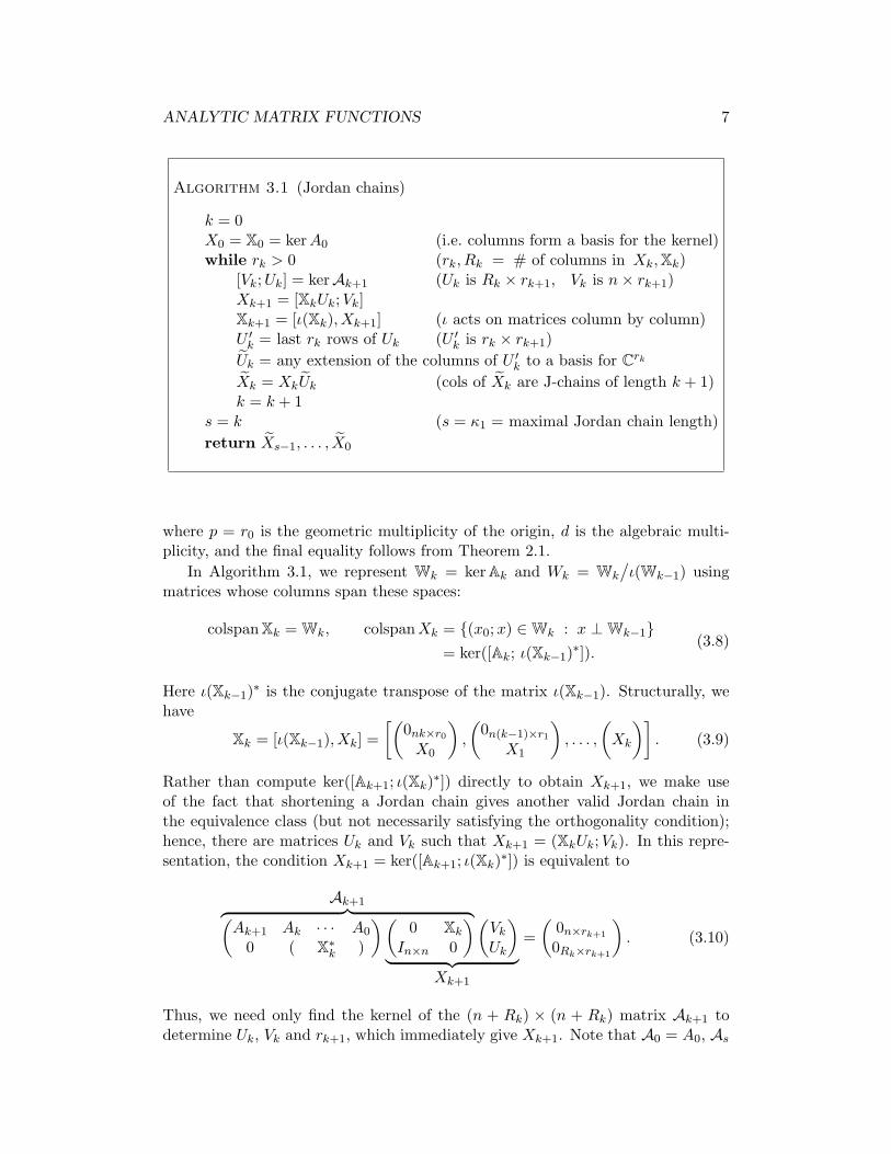
Algorithm 3.1 (Jordan chains)

k = 0X0 = X0 = kerA0 (i.e. columns form a basis for the kernel)while rk > 0 (rk, Rk = # of columns in Xk, Xk)

[Vk;Uk] = kerAk+1 (Uk is Rk × rk+1, Vk is n× rk+1)Xk+1 = [XkUk;Vk]Xk+1 = [ι(Xk), Xk+1] (ι acts on matrices column by column)U ′

k = last rk rows of Uk (U ′k is rk × rk+1)

Uk = any extension of the columns of U ′k to a basis for Crk

Xk = XkUk (cols of Xk are J-chains of length k + 1)k = k + 1

s = k (s = κ1 = maximal Jordan chain length)return Xs−1, . . . , X0

where p = r0 is the geometric multiplicity of the origin, d is the algebraic multi-plicity, and the final equality follows from Theorem 2.1.

In Algorithm 3.1, we represent Wk = ker Ak and Wk = Wk

/ι(Wk−1) using

matrices whose columns span these spaces:

colspan Xk = Wk, colspan Xk = {(x0;x) ∈ Wk : x ⊥ Wk−1}= ker([Ak; ι(Xk−1)∗]).

(3.8)

Here ι(Xk−1)∗ is the conjugate transpose of the matrix ι(Xk−1). Structurally, wehave

Xk = [ι(Xk−1), Xk] =[(

0nk×r0

X0

),

(0n(k−1)×r1

X1

), . . . ,

(Xk

)]. (3.9)

Rather than compute ker([Ak+1; ι(Xk)∗]) directly to obtain Xk+1, we make useof the fact that shortening a Jordan chain gives another valid Jordan chain inthe equivalence class (but not necessarily satisfying the orthogonality condition);hence, there are matrices Uk and Vk such that Xk+1 = (XkUk;Vk). In this repre-sentation, the condition Xk+1 = ker([Ak+1; ι(Xk)∗]) is equivalent to

Ak+1︷ ︸︸ ︷(Ak+1 Ak · · · A0

0 ( X∗k )

)(0 Xk

In×n 0

)(Vk

Uk

)︸ ︷︷ ︸

Xk+1

=(

0n×rk+1

0Rk×rk+1

). (3.10)

Thus, we need only find the kernel of the (n + Rk) × (n + Rk) matrix Ak+1 todetermine Uk, Vk and rk+1, which immediately give Xk+1. Note that A0 = A0, As

8 J. WILKENING

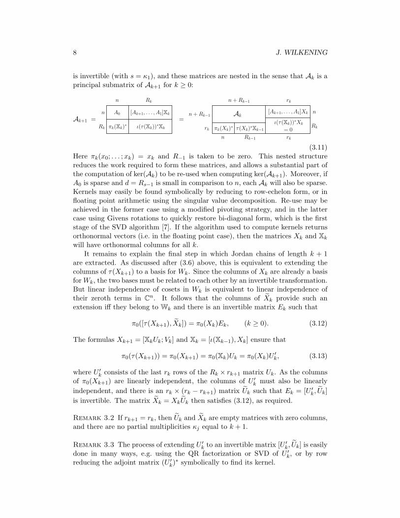
is invertible (with s = κ1), and these matrices are nested in the sense that Ak is aprincipal submatrix of Ak+1 for k ≥ 0:

τ(Xk)∗Xk−1

ι(τ(Xk))∗Xk

πk(Xk)∗

[Ak+1, . . . , A1]Xk

= 0

Ak

rkn + Rk−1

n + Rk−1

rk

n

Rk

rkn Rk−1

=Ak+1 =

[Ak+1, . . . , A1]Xk

ι(τ(Xk))∗Xk

A0

πk(Xk)∗

n

Rk

n Rk

(3.11)Here πk(x0; . . . ;xk) = xk and R−1 is taken to be zero. This nested structurereduces the work required to form these matrices, and allows a substantial part ofthe computation of ker(Ak) to be re-used when computing ker(Ak+1). Moreover, ifA0 is sparse and d = Rs−1 is small in comparison to n, each Ak will also be sparse.Kernels may easily be found symbolically by reducing to row-echelon form, or infloating point arithmetic using the singular value decomposition. Re-use may beachieved in the former case using a modified pivoting strategy, and in the lattercase using Givens rotations to quickly restore bi-diagonal form, which is the firststage of the SVD algorithm [7]. If the algorithm used to compute kernels returnsorthonormal vectors (i.e. in the floating point case), then the matrices Xk and Xk

will have orthonormal columns for all k.It remains to explain the final step in which Jordan chains of length k + 1

are extracted. As discussed after (3.6) above, this is equivalent to extending thecolumns of τ(Xk+1) to a basis for Wk. Since the columns of Xk are already a basisfor Wk, the two bases must be related to each other by an invertible transformation.But linear independence of cosets in Wk is equivalent to linear independence oftheir zeroth terms in Cn. It follows that the columns of Xk provide such anextension iff they belong to Wk and there is an invertible matrix Ek such that

π0([τ(Xk+1), Xk]) = π0(Xk)Ek, (k ≥ 0). (3.12)

The formulas Xk+1 = [XkUk;Vk] and Xk = [ι(Xk−1), Xk] ensure that

π0(τ(Xk+1)) = π0(Xk+1) = π0(Xk)Uk = π0(Xk)U ′k, (3.13)

where U ′k consists of the last rk rows of the Rk × rk+1 matrix Uk. As the columns

of π0(Xk+1) are linearly independent, the columns of U ′k must also be linearly

independent, and there is an rk × (rk − rk+1) matrix Uk such that Ek = [U ′k, Uk]

is invertible. The matrix Xk = XkUk then satisfies (3.12), as required.

Remark 3.2 If rk+1 = rk, then Uk and Xk are empty matrices with zero columns,and there are no partial multiplicities κj equal to k + 1.

Remark 3.3 The process of extending U ′k to an invertible matrix [U ′

k, Uk] is easilydone in many ways, e.g. using the QR factorization or SVD of U ′

k, or by rowreducing the adjoint matrix (U ′

k)∗ symbolically to find its kernel.

ANALYTIC MATRIX FUNCTIONS 9

Example 3.4 Let A(λ) =(

λ −λ2

λ2 0

)= A0 + λA1 + λ2A2. In this case, it is

simplest to compute Xk = ker([Ak; ι(Xk−1)∗]) directly, which yields

X0 =(

1 00 1

), X1 =

0100

, X2 =

0

1

1

0

0

0

, X3 = ∅8×0. (3.14)

Uk and Vk may be read off from Xk+1 = (XkUk;Vk): U0 = (0; 1), V0 = (0; 0),U1 = (1; 0; 1), V1 = (0; 0), U2 = ∅4×0, V2 = ∅2×0. We then obtain X0 = (1; 0),X1 = ∅4×0, X2 = X2, so a canonical system of root functions is

x1(λ) =(

λ1

), κ1 = 3, x2(λ) =

(10

), κ2 = 1. (3.15)

This example shows (with k = 1) that although the columns of τ(Xk+1) are guar-anteed to be linearly independent modulo ι(Wk−1), they need not satisfy the or-thogonality condition required to belong to colspan(Xk).

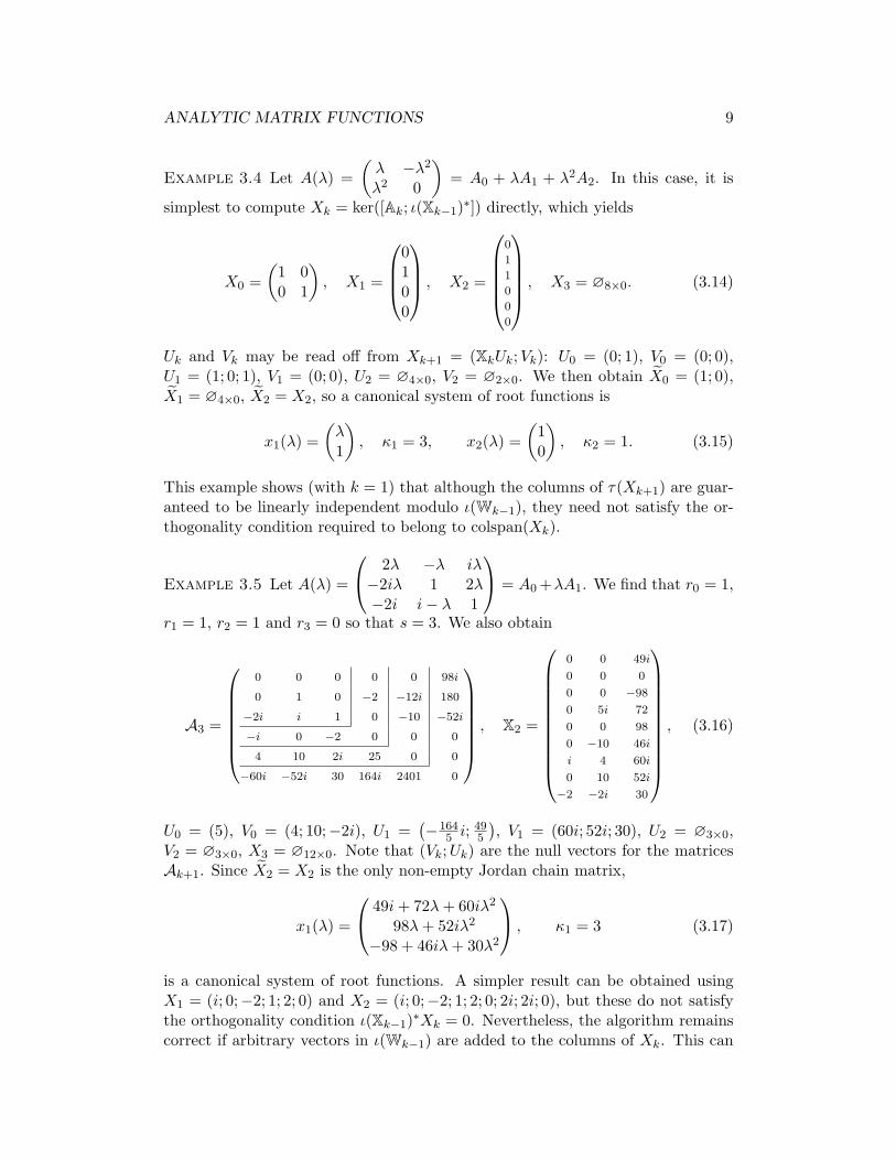
Example 3.5 Let A(λ) =

2λ −λ iλ−2iλ 1 2λ−2i i− λ 1

= A0 +λA1. We find that r0 = 1,

r1 = 1, r2 = 1 and r3 = 0 so that s = 3. We also obtain

A3 =

0 0 0 0 0 98i

0 1 0 −2 −12i 180

−2i i 1 0 −10 −52i

−i 0 −2 0 0 0

4 10 2i 25 0 0

−60i −52i 30 164i 2401 0

, X2 =

0 0 49i

0 0 0

0 0 −98

0 5i 72

0 0 98

0 −10 46i

i 4 60i

0 10 52i

−2 −2i 30

, (3.16)

U0 = (5), V0 = (4; 10;−2i), U1 =(−164

5 i; 495

), V1 = (60i; 52i; 30), U2 = ∅3×0,

V2 = ∅3×0, X3 = ∅12×0. Note that (Vk;Uk) are the null vectors for the matricesAk+1. Since X2 = X2 is the only non-empty Jordan chain matrix,

x1(λ) =

49i + 72λ + 60iλ2

98λ + 52iλ2

−98 + 46iλ + 30λ2

, κ1 = 3 (3.17)

is a canonical system of root functions. A simpler result can be obtained usingX1 = (i; 0;−2; 1; 2; 0) and X2 = (i; 0;−2; 1; 2; 0; 2i; 2i; 0), but these do not satisfythe orthogonality condition ι(Xk−1)∗Xk = 0. Nevertheless, the algorithm remainscorrect if arbitrary vectors in ι(Wk−1) are added to the columns of Xk. This can

10 J. WILKENING

be useful when the algorithm is run in exact arithmetic to reduce the size of therational entries in Ak and Xk by setting certain components of Xk to zero ratherthan requiring orthogonality; see Section 4.1. Different choices of the Xk lead todifferent matrices Ak and to different root functions xj(λ), but to the same termsin the Laurent expansion of A(λ)−1 in Section 4. In floating point arithmetic,requiring orthogonality seems most natural (and stable: see Appendix A).

4 Laurent expansion of A(λ)−1

As discussed in Section 2, the meromorphic behavior of A(λ)−1 is completelycharacterized by any canonical system of Jordan chains. In this section, we showhow to use the output of Algorithm 3.1 to efficiently compute an arbitrary numberof terms in the Laurent expansion of A(λ)−1b(λ) for any analytic (or meromorphic)vector function b(λ).

Let s = κ1 denote the maximal Jordan chain length. This is the first index forwhich Xs has no columns, Xs = ι(Xs−1), and the linear system

As

(vu

)=(

As As−1 · · · A0

0d×n ( X∗s−1 )

)(0sn×n Xs−1

In×n 0n×d

)(vu

)︸ ︷︷ ︸

(x0; . . . ;xs)

=(

b0

)(4.1)

is uniquely solvable and provides a linear mapping b 7→ (v;u) 7→ (x0; . . . ;xs). Hered = Rs−1 is the algebraic multiplicity of the origin, xk, b, v ∈ Cn and 0, u ∈ Cd.We will denote this mapping by

(x0; . . . ;xs) = solve(b) :=(

0 Xs−1

I 0

)A−1

s

(b0

). (4.2)

Suppose we wish to compute the first q + 1 terms in the Laurent expansion ofA(λ)−1b(λ), where b(λ) = b0 + λb1 + λ2b2 + · · · . Equation (2.11) shows thatthe most singular term in the expansion of A(λ)−1 is λ−s. If we can find anyx(λ) = x0 + λx1 + · · ·+ λq+sxq+s such that

A(λ)[λ−sx0 + · · ·+ λqxq+s] = b0 + · · ·+ λqbq + O(λq+1), (4.3)

thenA(λ)−1b(λ) = λ−s[x(λ) + O(λq+1)], (4.4)

so the terms x0, . . . , xq are correctly determined by solving (4.3). Matching likepowers of λ in (4.3), the xk should satisfy

Aq+s(x0; . . . ;xq+s) = (0; . . . ; 0; b0; . . . ; bq). (4.5)

To verify that this equation has a solution, observe that for q ≥ 0 we havedim ker A∗

q+s = dim ker A∗s−1; hence, the block structure of A∗

q+s ensures that

(x0; . . . ;xq+s) ∈ ker A∗q+s ⇒ xs = · · · = xq+s = 0, (q ≥ 0, xk ∈ Cn).

(4.6)

ANALYTIC MATRIX FUNCTIONS 11

As a result, the right-hand side of (4.5) belongs to ker(A∗q+s)

⊥, as required. Notethat any two solutions of (4.5) differ by at most a vector (0; . . . ; 0; ξ0; . . . ; ξs−1) ∈C(q+1+s)n with (ξ0; . . . ; ξs−1) ∈ colspan(Xs−1). This shows to what extent theterms xq+1, . . . , xq+s are left undetermined in (4.3).

Next we show how to bootstrap a solution to (4.5) by repeatedly solving thelinear system (4.1). Suppose k ≥ 1 and we have found vectors xi satisfying

Ak+s−1(x0; . . . ;xk+s−1) = (0; . . . ; 0; b0; . . . ; bk−1). (4.7)

For example, if k = 1 then such a solution is given by (x0; . . . ;xs) = solve(b0). Wewish to find corrections ξi such that

A0 0 · · · 0A1 A0 · · · 0· · · · · · · · · · · ·

Ak+s Ak+s−1 · · · A0

x0

· · ·xk−1

xk + ξ0

· · ·xk+s−1 + ξs−1

ξs

=

0...0b0...bk

. (4.8)

Moving the known vectors xi to the right hand side, this is equivalent to solving

Ak+s(0; . . . ; 0; ξ0; . . . ; ξs) = (0; . . . ; 0; bk −Ak+sx0 − · · · −A1xk+s−1). (4.9)

A solution of this equation is given by (ξ0; . . . ; ξs) = solve(bk −

∑k+sj=1 Ajxk+s−j

),

which we use to correct the xi in (4.8):

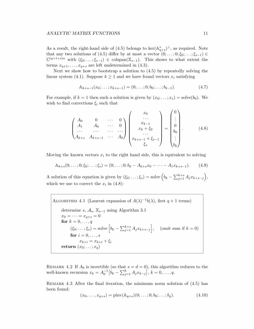
Algorithm 4.1 (Laurent expansion of A(λ)−1b(λ), first q + 1 terms)

determine s, As, Xs−1 using Algorithm 3.1x0 = · · · = xq+s = 0for k = 0, . . . , q

(ξ0; . . . ; ξs) = solve[bk −

∑k+sj=1 Ajxk+s−j

], (omit sum if k = 0)

for i = 0, . . . , sxk+i = xk+i + ξi

return (x0; . . . ;xq)

Remark 4.2 If A0 is invertible (so that s = d = 0), this algorithm reduces to thewell-known recursion xk = A−1

0

[bk −

∑kj=1 Ajxk−j

], k = 0, . . . , q.

Remark 4.3 After the final iteration, the minimum norm solution of (4.5) hasbeen found:

(x0, . . . , xq+s) = pinv(Aq+s)(0; . . . ; 0; b0; . . . ; bq). (4.10)

12 J. WILKENING

To see this, note that each time through the loop, (ξ1; . . . ; ξs) ⊥ Ws−1 due to thelast d equations of (4.1). By (3.9), we conclude that

ξs ⊥ W0 , (ξs−1; ξs) ⊥ W1 , . . . , (ξ1; . . . ; ξs) ⊥ Ws−1. (4.11)

But any (w0; . . . ;ws−1) ∈ Ws−1 also satisfies w0 ∈ W0, (w0;w1) ∈ W1, etc. Thuswe have

ξs

0...0

,

ξs−1

ξs

0...

, . . . ,

ξ1

ξ2...ξs

∈ (Ws−1)⊥. (4.12)

Since (xq+1; . . . ;xq+s) is a sum of such vectors, it belongs to (Ws−1)⊥, as claimed.

Remark 4.4 Several solutions may be found simultaneously by adding additionalcolumns to the vectors b(λ) and x(λ) above. In particular, replacing b(λ) by In×n

and x(λ) by Q(λ), we obtain A(λ)−1 = λ−s[Q0 + λQ1 + λ2Q2 + · · · ]. However, inpractice one often wishes to apply A(λ)−1 to a single vector function b(λ), in whichcase it is more efficient to carry out the procedure directly rather than computethe Laurent expansion of A(λ)−1 first. See Section 4.2 below.

Example 4.5 Let A(λ) be defined as in Example 3.5. Then s = 3 and A3, X2

were given in (3.16) above. For any q ≥ 2, Algorithm 4.1 gives

Q0 =

12 0 00 0 0i 0 0

, Q1 =

−i 0 − i2

−i 0 01 0 1

, Q2 =

1 − i2 −1

0 0 −1i 1 −i

, (4.13)

and Q3≤k≤q = 03×3, i.e. the Laurent expansion A(λ)−1 = λ−3[Q0 + λQ1 + · · · ]terminates at Q2.

4.1 Exact arithmetic and left Jordan chains

When Algorithm 4.1 is performed in infinite precision using rational numbers, thecost of each operation also grows with the problem size, so a straightforward O(n3)operation count will underestimate the running time. We have found that twomodifications can significantly reduce the size of the rational numbers that arisein the computation. The first modification involves the last Rk rows of Ak+1. Wedefine the first n rows as before, set vj = Ak+1(1:n, j) and define j1, . . . , jRk

to bethe first Rk indices encountered for which vj is linearly dependent on v1, . . . , vj−1.Then we define row n+ i of Ak+1 to have a one in column ji and zeros in all other

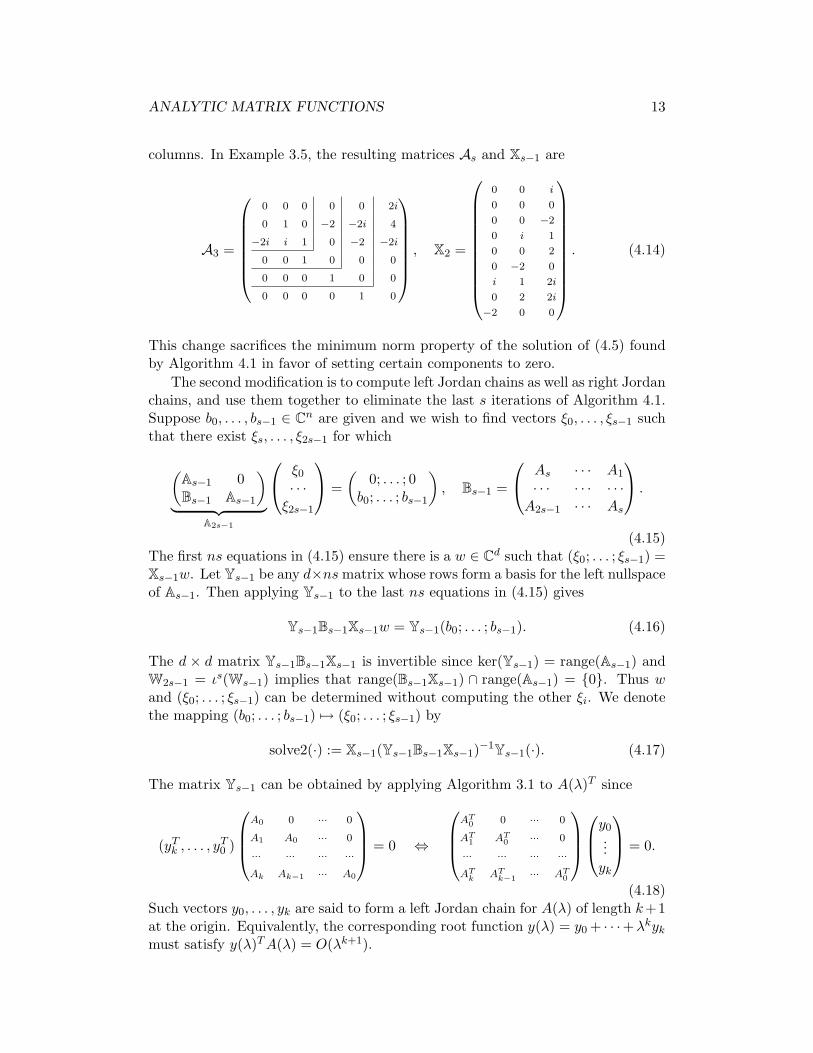
ANALYTIC MATRIX FUNCTIONS 13

columns. In Example 3.5, the resulting matrices As and Xs−1 are

A3 =

0 0 0 0 0 2i

0 1 0 −2 −2i 4

−2i i 1 0 −2 −2i

0 0 1 0 0 0

0 0 0 1 0 0

0 0 0 0 1 0

, X2 =

0 0 i

0 0 0

0 0 −2

0 i 1

0 0 2

0 −2 0

i 1 2i

0 2 2i

−2 0 0

. (4.14)

This change sacrifices the minimum norm property of the solution of (4.5) foundby Algorithm 4.1 in favor of setting certain components to zero.

The second modification is to compute left Jordan chains as well as right Jordanchains, and use them together to eliminate the last s iterations of Algorithm 4.1.Suppose b0, . . . , bs−1 ∈ Cn are given and we wish to find vectors ξ0, . . . , ξs−1 suchthat there exist ξs, . . . , ξ2s−1 for which

(As−1 0Bs−1 As−1

)︸ ︷︷ ︸

A2s−1

ξ0

· · ·ξ2s−1

=(

0; . . . ; 0b0; . . . ; bs−1

), Bs−1 =

As · · · A1

· · · · · · · · ·A2s−1 · · · As

.

(4.15)The first ns equations in (4.15) ensure there is a w ∈ Cd such that (ξ0; . . . ; ξs−1) =Xs−1w. Let Ys−1 be any d×ns matrix whose rows form a basis for the left nullspaceof As−1. Then applying Ys−1 to the last ns equations in (4.15) gives

Ys−1Bs−1Xs−1w = Ys−1(b0; . . . ; bs−1). (4.16)

The d × d matrix Ys−1Bs−1Xs−1 is invertible since ker(Ys−1) = range(As−1) andW2s−1 = ιs(Ws−1) implies that range(Bs−1Xs−1) ∩ range(As−1) = {0}. Thus wand (ξ0; . . . ; ξs−1) can be determined without computing the other ξi. We denotethe mapping (b0; . . . ; bs−1) 7→ (ξ0; . . . ; ξs−1) by

solve2(·) := Xs−1(Ys−1Bs−1Xs−1)−1Ys−1(·). (4.17)

The matrix Ys−1 can be obtained by applying Algorithm 3.1 to A(λ)T since

(yTk , . . . , yT

0 )

A0 0 ··· 0

A1 A0 ··· 0

··· ··· ··· ···Ak Ak−1 ··· A0

= 0 ⇔

AT

0 0 ··· 0

AT1 AT

0 ··· 0

··· ··· ··· ···AT

k ATk−1 ··· AT

0

y0

...yk

= 0.

(4.18)Such vectors y0, . . . , yk are said to form a left Jordan chain for A(λ) of length k+1at the origin. Equivalently, the corresponding root function y(λ) = y0 + · · ·+λkyk

must satisfy y(λ)T A(λ) = O(λk+1).

14 J. WILKENING

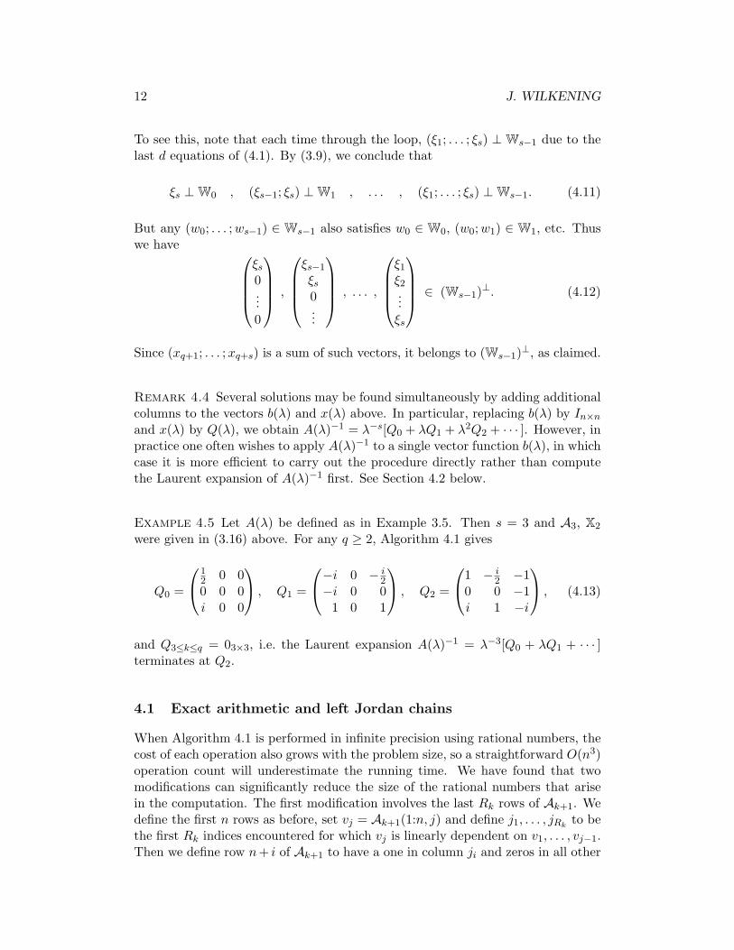
Algorithm 4.6 (Laurent expansion of A(λ)−1b(λ), first q + 1 terms)

determine s, As, Xs−1, Ys−1 using Algorithm 3.1if q < s− 1, increase it to q = s− 1x0 = · · · = xq = 0for k = 0, . . . , q − s (possibly empty loop)

(ξ0; . . . ; ξs) = solve[bk −

∑k+sj=1 Ajxk+s−j

], (omit sum if k = 0)

for i = 0, . . . , sxk+i = xk+i + ξi

(ξ0; . . . ; ξs−1) = solve2[bq−s+1

· · ·bq

−Aq+1 · · · A1

· · · · · · · · ·Aq+s · · · As

x0

· · ·xq

]for i = 1, . . . , s

xq−s+i = xq−s+i + ξi−1

return (x0; . . . ;xq)

Example 4.7 In Example 4.5 with X2 as in (4.14), we obtain the matrices

12

−i −1 i −1 0 −1 −i 0 0−1 0 −1 −i 0 0 0 0 0−i 0 0 0 0 0 0 0 0

,

Q0 0 0Q1 Q0 0Q2 Q1 Q0

(4.19)

for (Y2B2X2)−1Y2 and X2(Y2B2X2)−1Y2, respectively, with Qi as in (4.13).

Remark 4.8 Each column of Xs−1 has the form (0; . . . ; 0; x0; . . . ;xk) for some0 ≤ k ≤ s− 1. The corresponding column of Bs−1Xs−1 contains the coefficients ofthe truncated residual

b(λ) = λ−sA(λ)[λs−1−k(x0 + · · ·+ λkxk)] + O(λs), (4.20)

which satisfies A(λ)−1b(λ) = λ−1−k(x0 + · · ·+ λkxk) + O(1). See (2.12) above.

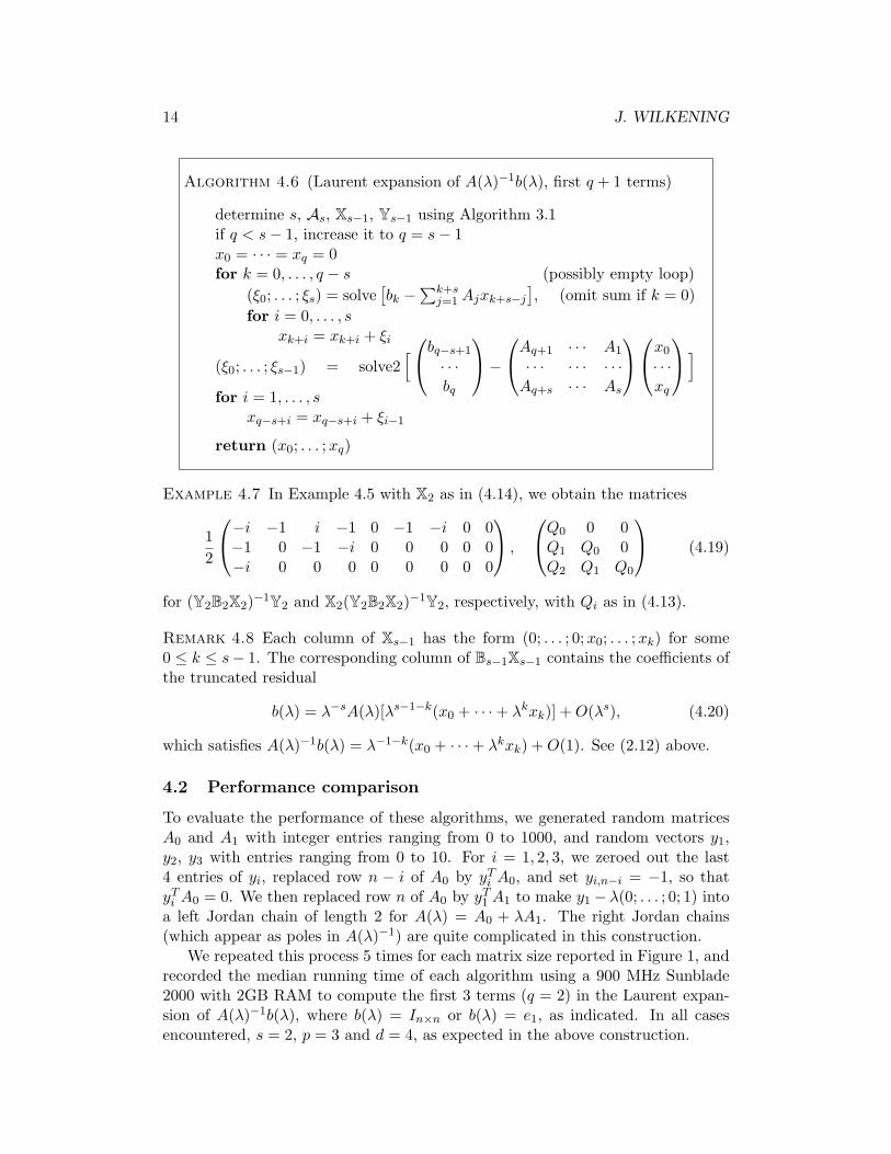
4.2 Performance comparison

To evaluate the performance of these algorithms, we generated random matricesA0 and A1 with integer entries ranging from 0 to 1000, and random vectors y1,y2, y3 with entries ranging from 0 to 10. For i = 1, 2, 3, we zeroed out the last4 entries of yi, replaced row n − i of A0 by yT

i A0, and set yi,n−i = −1, so thatyT

i A0 = 0. We then replaced row n of A0 by yT1 A1 to make y1 − λ(0; . . . ; 0; 1) into

a left Jordan chain of length 2 for A(λ) = A0 + λA1. The right Jordan chains(which appear as poles in A(λ)−1) are quite complicated in this construction.

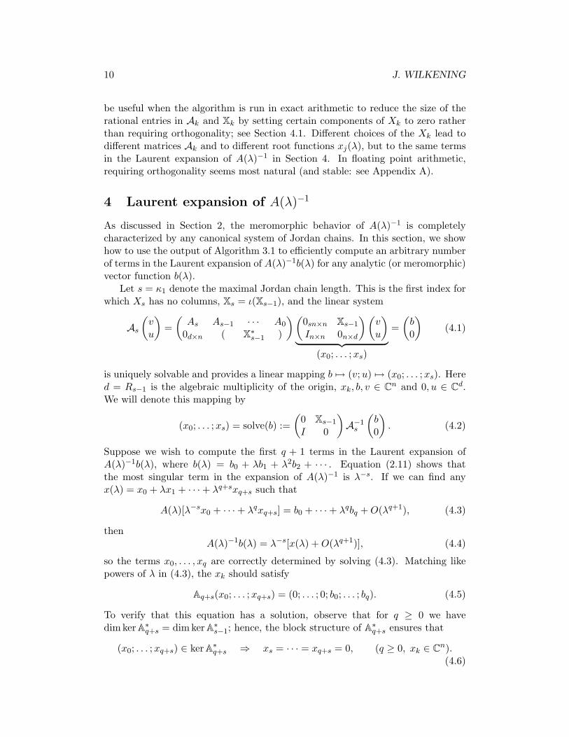
We repeated this process 5 times for each matrix size reported in Figure 1, andrecorded the median running time of each algorithm using a 900 MHz Sunblade2000 with 2GB RAM to compute the first 3 terms (q = 2) in the Laurent expan-sion of A(λ)−1b(λ), where b(λ) = In×n or b(λ) = e1, as indicated. In all casesencountered, s = 2, p = 3 and d = 4, as expected in the above construction.

ANALYTIC MATRIX FUNCTIONS 15

101 102 103

10−2

10−1

100

101

102

103

104

Comparison of various algorithms

matrix size (n)

runn

ing

time

(in s

econ

ds)

Smith form

symbolic linear solve

Alg. 4.

6 (ex

act a

rithmeti

c)

Alg. 4.1

(floa

ting po

int)

b(λ)=I

b(λ)=e 1

b(λ)=e1

b(λ)=I

with truncation

pinv(

A 4) (f

loating

point)

slopes of lines (from left to right):10.4, 3.8, 3.7, 3.8, 3.4, 3.1, 2.9, 2.9

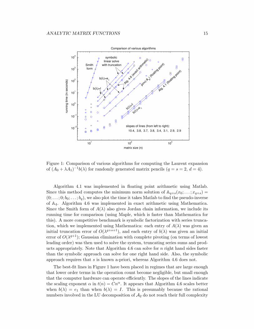
Figure 1: Comparison of various algorithms for computing the Laurent expansionof (A0 + λA1)−1b(λ) for randomly generated matrix pencils (q = s = 2, d = 4).

Algorithm 4.1 was implemented in floating point arithmetic using Matlab.Since this method computes the minimum norm solution of Aq+s(x0; . . . ;xq+s) =(0; . . . ; 0; b0; . . . ; bq), we also plot the time it takes Matlab to find the pseudo-inverseof A4. Algorithm 4.6 was implemented in exact arithmetic using Mathematica.Since the Smith form of A(λ) also gives Jordan chain information, we include itsrunning time for comparison (using Maple, which is faster than Mathematica forthis). A more competitive benchmark is symbolic factorization with series trunca-tion, which we implemented using Mathematica: each entry of A(λ) was given aninitial truncation error of O(λq+s+1), and each entry of b(λ) was given an initialerror of O(λq+1); Gaussian elimination with complete pivoting (on terms of lowestleading order) was then used to solve the system, truncating series sums and prod-ucts appropriately. Note that Algorithm 4.6 can solve for n right hand sides fasterthan the symbolic approach can solve for one right hand side. Also, the symbolicapproach requires that s is known a-priori, whereas Algorithm 4.6 does not.

The best-fit lines in Figure 1 have been placed in regimes that are large enoughthat lower order terms in the operation count become negligible, but small enoughthat the computer hardware can operate efficiently. The slopes of the lines indicatethe scaling exponent α in t(n) = Cnα. It appears that Algorithm 4.6 scales betterwhen b(λ) = e1 than when b(λ) = I. This is presumably because the rationalnumbers involved in the LU decomposition of A2 do not reach their full complexity

16 J. WILKENING

until the final stages of the factorization, whereas for b(λ) = I, all O(n3) operationsof the back-solve stage involve these large rational numbers. We also see that thefloating point algorithm scales as O(n3), as predicted by a straightforward floatingpoint operation count. In many cases where A(0) has special structure, it shouldbe possible to make use of the fact that As contains A(0) as a principal submatrixto further improve this scaling.

A Numerical stability in floating point arithmetic

In this section we will show that the algorithms presented in this paper are forwardstable in floating point arithmetic with a condition number that depends on howclose A(λ) is to an even more singular analytic matrix function. This is possiblebecause we have specified the location of the eigenvalue of interest (e.g. the origin)as part of the problem statement. Thus, we have to know more about the matrixthan can be determined by looking at a numerical approximation of it — we haveto know that A(0) is exactly singular. In particular, we do not claim to be ableto compute the Jordan canonical form of a matrix in a stable way unless theeigenvalues are known a-priori, or can be determined algebraically (using exactarithmetic for that part of the calculation). If the multiplicities can be determinedalgebraically, the eigenvalues can be computed in floating point arithmetic (usingextra precision if necessary), but there is no way to determine affirmatively that acluster of eigenvalues should coalesce using floating point arithmetic alone.

Finding the Jordan chains of an analytic matrix function at the origin is ageneralization of the familiar problem of finding the kernel of an n× n matrix A,which is solved numerically as follows. The user supplies a numerical approxima-tion A of A and a tolerance σthresh. The singular value decomposition A = UΣV ∗

is then computed and the right singular vectors corresponding to singular valuesσj < σthresh are returned as a basis for the kernel. This procedure is forward stabledue to the backward stability of the SVD algorithm:

Theorem A.1 (Backward stability of the SVD). Let A be a floating point repre-sentable n × n matrix. There is a (small) constant C independent of A (and n)such that the result of computing the SVD of A in floating point arithmetic (us-ing Givens rotations for the bi-diagonal reduction process) is the exact SVD of anearby matrix A satisfying

A = U ΣV ∗, ‖A− A‖ ≤ Cn2ε‖A‖, (A.1)

where ε is machine precision and the matrix multiplication is in exact arithmetic.

Remark A.2 The matrices U and V are stored implicitly as compositions ofGivens rotations so they are exactly orthogonal. If Householder reflections areused in the reduction to bidiagonal form, the bound on the right hand side of(A.1) involves the Frobenius norm instead of the 2-norm. This would requireminor modifications of the analysis below.

ANALYTIC MATRIX FUNCTIONS 17

Theorem A.3 (Forward stability of computing nullspaces). Suppose A = UΣV ∗

is an n×n matrix with dim kerA = p ≥ 0. Let gap = σn−p be the smallest non-zerosingular value of A, and suppose a tolerance σthresh is given such that

σthresh ≤13

gap . (A.2)

Let α ≥ ‖A‖, γ > 0, and A be any floating point representable matrix satisfying

‖A−A‖ ≤ γαn2ε, γn2ε ≤ 1/3. (A.3)

Let A = U ΣV ∗ be the result of computing the SVD of A in floating point arithmetic.Then

A = A + E, ‖E‖ ≤(

γ +43C

)αn2ε, |σj − σj | ≤ ‖E‖, (1 ≤ j ≤ n),

(A.4)where C is the backward stability constant of the SVD algorithm from (A.1). Inparticular, if

ε <σthresh

(γ + 4C/3)αn2, (A.5)

the number of singular values satisfying σj < σthresh is p and there is an orthogonaln× p nullspace matrix X for A such that

‖X −X‖ ≤ 1.1‖E‖gap

, AX = 0, X∗X = Ip×p, (A.6)

where X is the numerical nullspace matrix consisting of the last p columns of V(stored implicitly using Givens rotations). Finally, if we explicitly compute thematrix entries of X in floating point arithmetic, we obtain a matrix X satisfying‖X − X‖ ≤ 1

2Cn2ε as well as

‖X −X‖ ≤ Kε, K = (1.1γ + 2C)n2 α

gap. (A.7)

Remark A.4 The bound (A.4) on the singular values follows from Weyl’s the-orem [7]. The bound (A.6) on X follows from the “sin 2Θ” theorem [6] on theperturbation of invariant subspaces. The constant 1.1 in (A.6) is related to thechoice of 1/3 in (A.2), for if 0 ≤ θ ≤ π

4 and 12 sin 2θ ≤ 1

3 then 2 sin θ2 ≤

1.12 sin 2θ.

The requirement γn2ε ≤ 1/3 is satisfied automatically if (A.2) and (A.5) hold(since gap ≤ α). The constant α can be any convenient bound on ‖A‖ (including‖A‖ itself). The purpose of γ is to quantify the effect of starting with a poorapproximation A of A when analyzing Algorithm 3.1 below.

In summary, given A and and a tolerance σthresh satisfying (A.2), the nullspacematrix X computed in floating point arithmetic is close to an exact nullspacematrix X as long as ε satisfies (A.5), and the error can be made arbitrarily smallby taking ε → 0. Thus, computing nullspaces is forward stable in floating point

18 J. WILKENING

arithmetic with condition number K proportional to n2‖A‖/ gap. Note that anyperturbation of A that decreases the dimension of the kernel will have a muchlarger condition number due to the small, non-zero singular value(s) created bythe perturbation.

Except for the last step where we explicitly compute the matrix entries of X,this procedure for computing the nullspace is also backward stable as zeroing outthe p smallest singular values σj will not change A very much; however, backwardstability is less useful than forward stability when the underlying problem dependsdiscontinuously on the matrix entries. For example, the algorithm “return then × 0 empty matrix X” is also backward stable as there are invertible matricesarbitrarily close to any singular matrix.

Before analyzing the stability of Algorithm 3.1, it is instructive to consider thenaive algorithm employing the SVD to compute the nullspace matrices Xk directlyfrom Ak for k = 0, 1, 2, . . . , until Rk = dim ker Ak stops increasing. We identifythe maximal Jordan chain length s as the first k for which Rk = Rk−1 (with R−1

taken to be 0). The matrix Xs−1 then contains all the Jordan chain informationfor A(λ). Setting γ = 1 and α = ‖As−1‖ in (A.7), we see that a natural candidatefor the condition number of this problem is

Knaive =(1.1 + 2C)s2n2‖As−1‖

gapnaives−1

, (A.8)

where gapnaivek is the smallest non-zero singular value of Ak. The bounds in (A.4)

above imply that given A(λ) of maximal Jordan chain length s at the origin anda tolerance

σthresh ≤ min0≤k≤s

(13

gapnaivek

), (A.9)

the naive algorithm will compute the dimensions R0, . . . , Rs correctly as long as

ε <σthresh

(1 + 4C/3)(s + 1)2n2‖As‖(A.10)

and as long as our numerical approximations Ak of the coefficients of A(λ) leadto augmented matrices that satisfy ‖Ak − Ak‖ ≤ n2(k + 1)2ε‖Ak‖ for 0 ≤ k ≤ s.Moreover, the computed nullspace Xs−1 will be close to an exact nullspace matrixXs−1 for As−1:

‖Xs−1 − Xs−1‖ ≤ Knaive ε. (A.11)

Thus, the naive algorithm is forward stable with condition number Knaive. How-ever, this analysis overlooks one important detail: computing the nullspace of As−1

using the SVD will not respect the Jordan chain structure of this nullspace; hence,there are likely to be internal inconsistencies when we try to extract Jordan chainsfrom Xs−1. This is illustrated in the following two examples:

Example A.5 Let A(λ) = P

1 + λ 0 00 a 03λ 0 λ2

Q∗, where P and Q are randomly

generated orthogonal matrices and a = 10−8. (The purpose of P and Q is to

ANALYTIC MATRIX FUNCTIONS 19

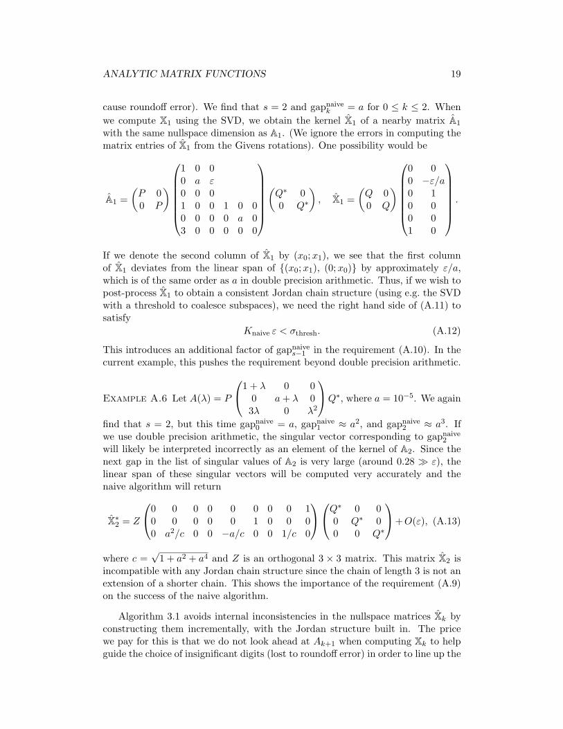
cause roundoff error). We find that s = 2 and gapnaivek = a for 0 ≤ k ≤ 2. When

we compute X1 using the SVD, we obtain the kernel X1 of a nearby matrix A1

with the same nullspace dimension as A1. (We ignore the errors in computing thematrix entries of X1 from the Givens rotations). One possibility would be

A1 =(

P 00 P

)

1 0 00 a ε0 0 01 0 0 1 0 00 0 0 0 a 03 0 0 0 0 0

(

Q∗ 00 Q∗

), X1 =

(Q 00 Q

)

0 00 −ε/a0 10 00 01 0

.

If we denote the second column of X1 by (x0;x1), we see that the first columnof X1 deviates from the linear span of {(x0;x1), (0; x0)} by approximately ε/a,which is of the same order as a in double precision arithmetic. Thus, if we wish topost-process X1 to obtain a consistent Jordan chain structure (using e.g. the SVDwith a threshold to coalesce subspaces), we need the right hand side of (A.11) tosatisfy

Knaive ε < σthresh. (A.12)

This introduces an additional factor of gapnaives−1 in the requirement (A.10). In the

current example, this pushes the requirement beyond double precision arithmetic.

Example A.6 Let A(λ) = P

1 + λ 0 00 a + λ 03λ 0 λ2

Q∗, where a = 10−5. We again

find that s = 2, but this time gapnaive0 = a, gapnaive

1 ≈ a2, and gapnaive2 ≈ a3. If

we use double precision arithmetic, the singular vector corresponding to gapnaive2

will likely be interpreted incorrectly as an element of the kernel of A2. Since thenext gap in the list of singular values of A2 is very large (around 0.28 � ε), thelinear span of these singular vectors will be computed very accurately and thenaive algorithm will return

X∗2 = Z

0 0 0 0 0 0 0 0 10 0 0 0 0 1 0 0 00 a2/c 0 0 −a/c 0 0 1/c 0

Q∗ 0 00 Q∗ 00 0 Q∗

+O(ε), (A.13)

where c =√

1 + a2 + a4 and Z is an orthogonal 3 × 3 matrix. This matrix X2 isincompatible with any Jordan chain structure since the chain of length 3 is not anextension of a shorter chain. This shows the importance of the requirement (A.9)on the success of the naive algorithm.

Algorithm 3.1 avoids internal inconsistencies in the nullspace matrices Xk byconstructing them incrementally, with the Jordan structure built in. The pricewe pay for this is that we do not look ahead at Ak+1 when computing Xk to helpguide the choice of insignificant digits (lost to roundoff error) in order to line up the

20 J. WILKENING

subspaces at the next iteration (to find chains of length k+1). Thus, Algorithm 3.1may require more precision than the naive algorithm to find long chains, but thenaive algorithm will require additional precision to make sense of the nullspaces itfinds (and to avoid finding too many null vectors).

Examples A.5 and A.6 above are cases where the naive algorithm fails in doubleprecision arithmetic while Algorithm 3.1 succeeds (with typically 9 correct digitsin X in the former case and 7 in the latter). If we set a = 10−8 and replace thesecond column of A(λ) by (0; a;λ), then the naive algorithm will succeed in doubleprecision arithmetic while Algorithm 3.1 will fail to find the chain of length 2. Ifwe instead replace the second column by (0; a + λ;λ), then both algorithms willfail unless extra precision is used: the naive algorithm will find a spurious chainof length 3 while Algorithm 3.1 will fail to find the chain of length 2. In all cases,both algorithms will succeed once ε is reduced to satisfy (A.12) or (A.28) below.

These examples can be understood by noting that the error in computing kerA0

is overwhelmingly in the direction of the second right singular vector v2 = Q(:, 2)due to the large gap between σ1 and σ2 and the small gap between σ2 and σ3 = 0.The requirements on ε for the success of the algorithms (and in particular thequantities gapnaive

k ) depend on where A1 maps v2. The examples above illustrateseveral of the possibilities.

We now prove that Algorithm 3.1 is forward stable in floating point arithmetic.Suppose A(λ) is exactly singular at the origin with maximal Jordan chain length s.We define

α0 = ‖A0‖, (A.14)

αk =(1 + ‖A0‖2 + · · ·+ ‖Ak‖2

)1/2, (0 ≤ k ≤ s), (A.15)

σ(k)j = jth singular value of Ak,

(σ

(k)1 ≥ · · · ≥ σ

(k)n+Rk−1

)(A.16)

gapk = σ(k)n+Rk−1−rk

= smallest non-zero singular value of Ak. (A.17)

The quantities αk are convenient upper bounds for ‖Ak‖, and, as before, R−1 = 0.Note that σ

(k)j and gapk are independent of which orthogonal matrices Xk and Xk

we use to represent the kernels. Also note that gaps is the smallest singular valueof As, which is invertible. The user must supply a threshold σthresh for computingnullspaces that satisfies

σthresh ≤13

(min

0≤k≤sgapk

). (A.18)

This requirement is often much less strict than (A.9). We assume that numericalapproximations of A0,. . . ,As are known to a tolerance

‖Ak −Ak‖ ≤ n2ε ‖Ak‖, (0 ≤ k ≤ s). (A.19)

The first step of the algorithm is to compute the kernel X0 of A0 as describedabove. In light of (A.19) and (A.14), Theorem A.3 implies that X0 satisfies

‖X0 − X0‖ ≤ (1.1 + 2C)n2 α0

gap0

ε,

(ε <

σthresh

(1 + 4C/3)α0 n2

). (A.20)

ANALYTIC MATRIX FUNCTIONS 21

Next we choose δ > 0 (to be determined later) and formulate the induction hy-pothesis

‖Xk − Xk‖ ≤ Ck(n + Rk−1)2ε ≤ δ. (A.21)

From (A.20), we know C0 = (1.1 + 2C)α0/ gap0 works when k = 0. Our goal isto derive a recursion for Ck that ensures that s is computed correctly, and that(A.21) holds for 1 ≤ k ≤ s− 1 as well. To this end, we compute

Ak+1 = fl[(

Ak+1 Ak · · · A0

0 ( X∗k )

)(0 Xk

In×n 0

)], (A.22)

where fl(·) indicates that the calculation is done in floating point arithmetic, anduse (A.21) to conclude

‖Ak+1 −Ak+1‖ ≤ γkαk+1(n + Rk)2ε, γk = (1 + δ)2[(k + 2) + 2Ck]. (A.23)

Next we compute [Vk; Uk] = fl(ker Ak+1

)and use Theorem A.3 to determine∥∥[Vk; Uk]− [Vk;Uk]

∥∥ ≤ (1.1γk + 2C)αk+1

gapk+1

(n + Rk)2ε. (A.24)

Finally, we compute

Xk+1 = fl[(

0 Xk

I 0

)(Vk

Uk

)], Xk+1 =

[(0

Xk

),

(Xk+1

)](A.25)

to obtain∥∥Xk+1 − Xk+1

∥∥ ≤ ((2 + δ)Ck + (1 + δ)2 +[1.1γk + 2C

] αk+1

gapk+1

)︸ ︷︷ ︸

Ck+1

(n + Rk)2ε.

We now select δ = 0.1 and use the fact that αk+1 ≥ gapk+1 to obtain a simplerrecursion (with larger terms):

Ck+1 =(

5Ck +43(k + 3) + 2C

)αk+1

gapk+1

, C0 = (1.1 + 2C)α0

gap0

. (A.26)

This recursion can be solved explicitly:

Ck =[5k+1 − 1

2C +

13160

5k − 1312− k

3

]αk

gapk

· · · α0

gap0

, (A.27)

which yields γk as well. In order for this analysis to be valid (and to determinethat k = s is the first index for which Ak is invertible), we require

ε < min(

δ

Cs−1(n + Rs−2)2,

σthresh

(γs−1 + 4C/3)αs(n + Rs−1)2

). (A.28)

The bounds on ‖Uk − Uk‖ and ‖Vk − Vk‖ in (A.24) can now be used to deriveerror estimates for the extracted Jordan chains Xk in Algorithm 3.1. The bound(A.23) on ‖As−As‖ ensures that Algorithm 4.1 is forward stable in floating pointarithmetic once b(λ) and the number of desired terms q in the Laurent expansionof A(λ)−1b(λ) have been specified.

22 J. WILKENING

Remark A.7 The exponential dependence of Ck on k in (A.28) is not likely tocause difficulty as problems with Jordan chain lengths longer than s = 3 are veryrare in practice. Of more concern is the fact that the ratios αk/ gapk multiply fromone iteration to the next. Example A.6 above shows that this should be expectedfrom a general (i.e. worst case) analysis. In that example, the quantities gapk

are all equal to a while gapnaivek ≈ ak+1 for 0 ≤ k ≤ 2. Example A.5 shows that

sometimes Algorithm 3.1 will perform better than predicted by this worst caseanalysis — it depends how the errors in Xk propagate through the coefficients Aj

when Ak+1 is formed in (A.22). However, a general analysis that keeps track ofthe directions of the errors as well as their norms would be difficult.

In summary, the error in the quantities computed in Algorithms 3.1 and 4.1using floating point arithmetic can be made arbitrarily small (relative to theirnearest counterparts in exact arithmetic) by taking ε → 0. Moreover, the con-vergence rates are linear in ε with constants that depend on the distance to aneven more singular analytic matrix function (i.e. on the sizes of the ratios αk

gapk,

0 ≤ k ≤ s− 1):

‖Xs−1 − Xs−1‖ ≤ Kε, K = Cs−1(n + Rs−2)2. (A.29)

The convergence is linear because we have specified the location of the singularity(the origin) in advance. In some problems, the zeros of ∆(λ) = det A(λ) must alsobe found, in which case we recommend Davies’ method [5] for locating the zerosof an analytic function using contour integration techniques. But if ∆(λ) has azero of order d at λ0, roundoff error is likely to split this zero like the dth root ofε rather than linearly, making these zeros difficult to compute.

It is often possible to use the methods of this paper to stabilize the problemof finding these zeros. For example, in the corner singularities problem describedin the introduction, it is very common for ∆(λ) to have zeros at the integers; thecorresponding singular functions are polynomials. If another zero λ1 of ∆(λ) isclose to such an integer λ0, Davies’ method will likely give inaccurate results as thezeros will interfere with each other. But if we first compute a canonical system ofJordan chains at the integer λ0, we learn the order d of the zero of ∆(λ) at λ0 usingan O(ε) method; we can then find λ1 using Davies’ method on ∆(λ)(λ − λ0)−d,which also gives O(ε) accuracy if λ1 is a simple zero. In this way we can findparasitic zeros near a known (possibly multiple) zero with high accuracy.

References

[1] K. E. Avrachenkov, M. Haviv, and P. G. Howlett. Inversion of analytic ma-trix functions that are singular at the origin. SIAM J. Matrix Anal. Appl.,22(4):1175–1189, 2001.

[2] H. Baumgartel. Analytic Perturbation Theory for Matrices and Operators.Birkhauser, Basel, 1985.

ANALYTIC MATRIX FUNCTIONS 23

[3] S. L. Campbell. Singular systems of differential equations II, volume 61 ofResearch Notes in Mathematics. Pitman, London, 1982.

[4] Martin Costabel and Monique Dauge. Construction of corner singularities forAgmon-Douglis-Nirenberg elliptic systems. Math. Nachr., 162:209–237, 1993.

[5] B. Davies. Locating the zeros of an analytic function. J. Comput. Phys.,66(1):36–49, 1986.

[6] C. Davis and W. M. Kahan. The rotation of eigenvectors by a perturbation.III. SIAM J. Numer. Anal., 7(1):1–46, 1970.

[7] James W. Demmel. Applied Numerical Linear Algebra. SIAM, Philadelphia,1997.

[8] A. Edelman, E. Elmroth, and B. Kagstrom. A geometric approach to per-turbation theory of matrices and matrix pencils, part I: versal deformations.SIAM J. Matrix Anal. Appl., 18(3):653–692, 1997.

[9] I. Gohberg, M. A. Kaashoek, and F. van Schagen. On the local theory ofregular analytic matrix functions. Linear Algebra Appl., 182:9–25, 1993.

[10] I. Gohberg, P. Lancaster, and L. Rodman. Matrix Polynomials. AcademicPress, New York, 1982.

[11] M. Haviv and Y. Ritov. On series expansions and stochastic matrices. SIAMJ. Matrix Anal. Appl., 14(3):670–676, 1993.

[12] M. V. Keldysh. On the characteristic values and characteristic functions ofcertain classes of non-selfadjoint equations. Dokl. Akad. Nauk USSR (Rus-sian), 77:11–14, 1951. English transl. in [15].

[13] P. Lancaster. Inversion of lambda-matrices and application to the theory oflinear vibrations. Arch. Rational Mech. Anal., 6(2):105–114, 1960.

[14] C. E. Langenhop. The Laurent expansion for a nearly singular matrix. LinearAlgebra Appl., 4:329–340, 1971.

[15] A. S. Markus. Introduction to the Spectral Theory of Polynomial OperatorPencils, volume 71 of Translations of Mathematical Monographs. AmericalMathematical Society, Providence, 1988.

[16] M. K. Sain and J. L. Massey. Invertibility of linear time-invariant dynamicalsystems. IEEE Trans. Automat. Control, (2):141–149, 1969.

[17] P. Schweitzer and G. W. Stewart. The Laurent expansion of pencils that aresingular at the origin. Linear Algebra Appl., 183:237–254, 1993.