COMP 182 Algorithmic Thinking Markov Chains andnakhleh/COMP182/MarkovChainsAndHMMs.pdfMarkov Chains...

COMP 182 Algorithmic Thinking

Markov Chains and Hidden Markov Models

Luay NakhlehComputer ScienceRice University

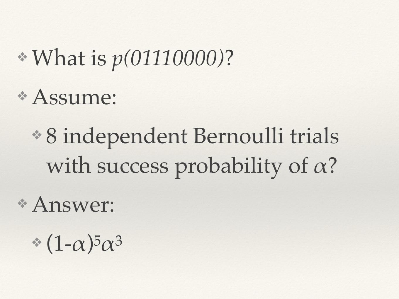
❖ What is p(01110000)? ❖ Assume:

❖ 8 independent Bernoulli trials with success probability of α?

❖ Answer:❖ (1-α)5α3

❖However, what if the assumption of independence doesn’t hold?

❖That is, what if the outcome in a Bernoulli trial depends on the outcomes of the trials the preceded it?

Markov Chains

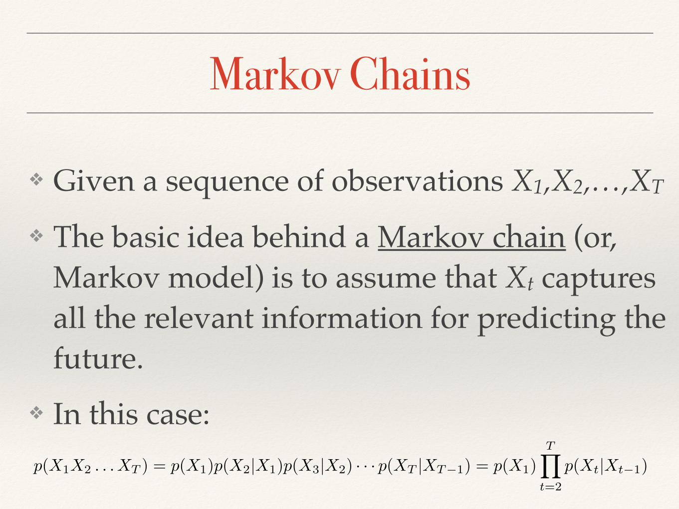
❖ Given a sequence of observations X1,X2,…,XT

❖ The basic idea behind a Markov chain (or, Markov model) is to assume that Xt captures all the relevant information for predicting the future.

❖ In this case: p(X1X2 . . . XT ) = p(X1)p(X2|X1)p(X3|X2) · · · p(XT |XT�1) = p(X1)

TY

t=2

p(Xt|Xt�1)

Markov Chains

❖ When Xt is discrete, so Xt∈{1,…,K}, the conditional distribution p(Xt|Xt-1) can be written as a K×K matrix, known as the transition matrix A, where Aij=p(Xt=j|Xt-1=i) is the probability of going from state i to state j.

❖ Each row of the matrix sums to one, so this is called a stochastic matrix.

Markov Chains

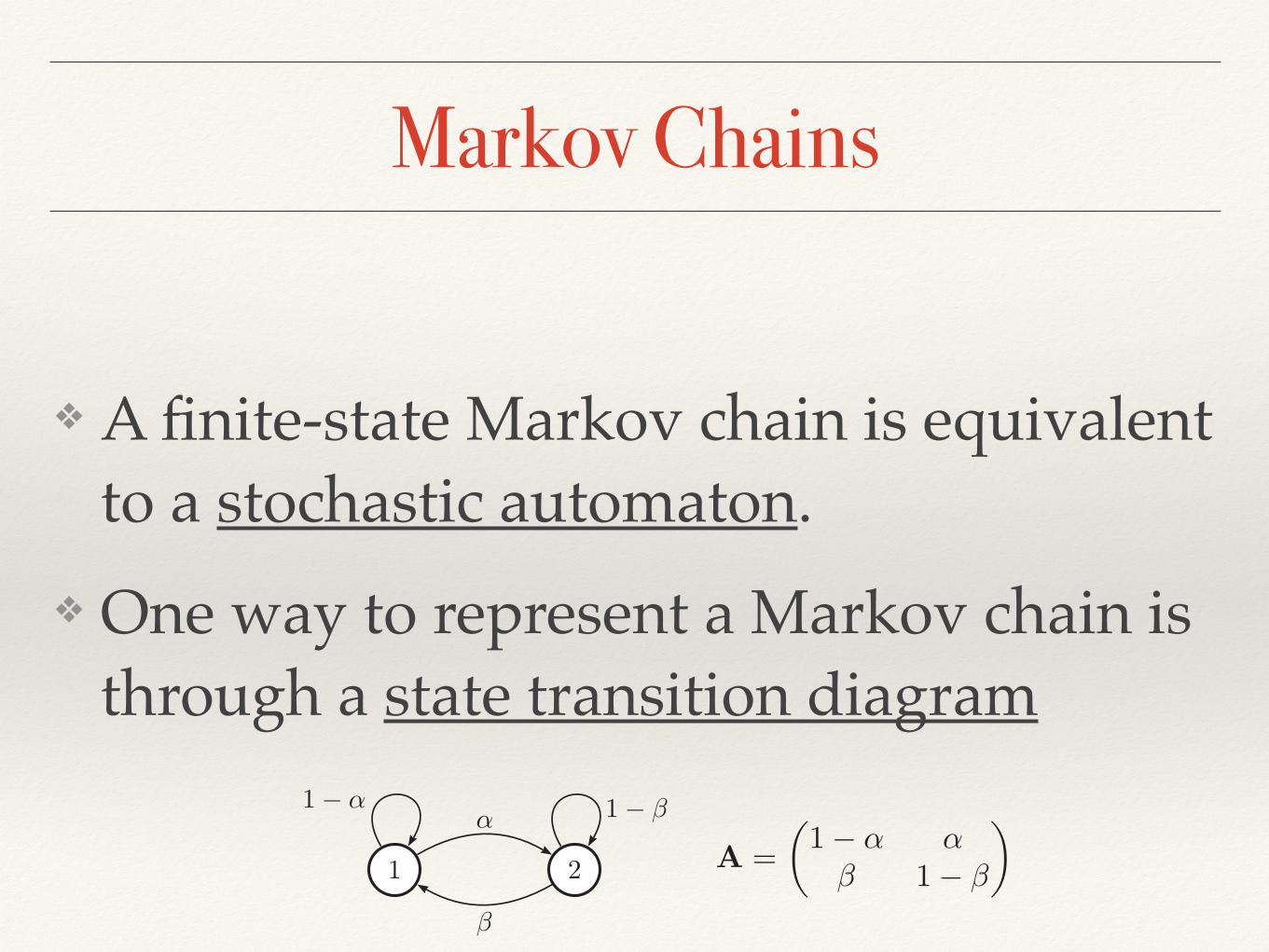
❖ A finite-state Markov chain is equivalent to a stochastic automaton.

❖ One way to represent a Markov chain is through a state transition diagram590 Chapter 17. Markov and hidden Markov models

1 2

α

β

1− α 1− β

(a)

1 2 3

A12 A23

A11 A22 A33

(b)

Figure 17.1 State transition diagrams for some simple Markov chains. Left: a 2-state chain. Right: a3-state left-to-right chain.

A stationary, finite-state Markov chain is equivalent to a stochastic automaton. It is commonto visualize such automata by drawing a directed graph, where nodes represent states and arrowsrepresent legal transitions, i.e., non-zero elements of A. This is known as a state transitiondiagram. The weights associated with the arcs are the probabilities. For example, the following2-state chain

A =

(1− α αβ 1− β

)(17.2)

is illustrated in Figure 17.1(left). The following 3-state chain

A =

⎛

⎝A11 A12 00 A22 A23

0 0 1

⎞

⎠ (17.3)

is illustrated in Figure 17.1(right). This is called a left-to-right transition matrix, and is com-monly used in speech recognition (Section 17.6.2).

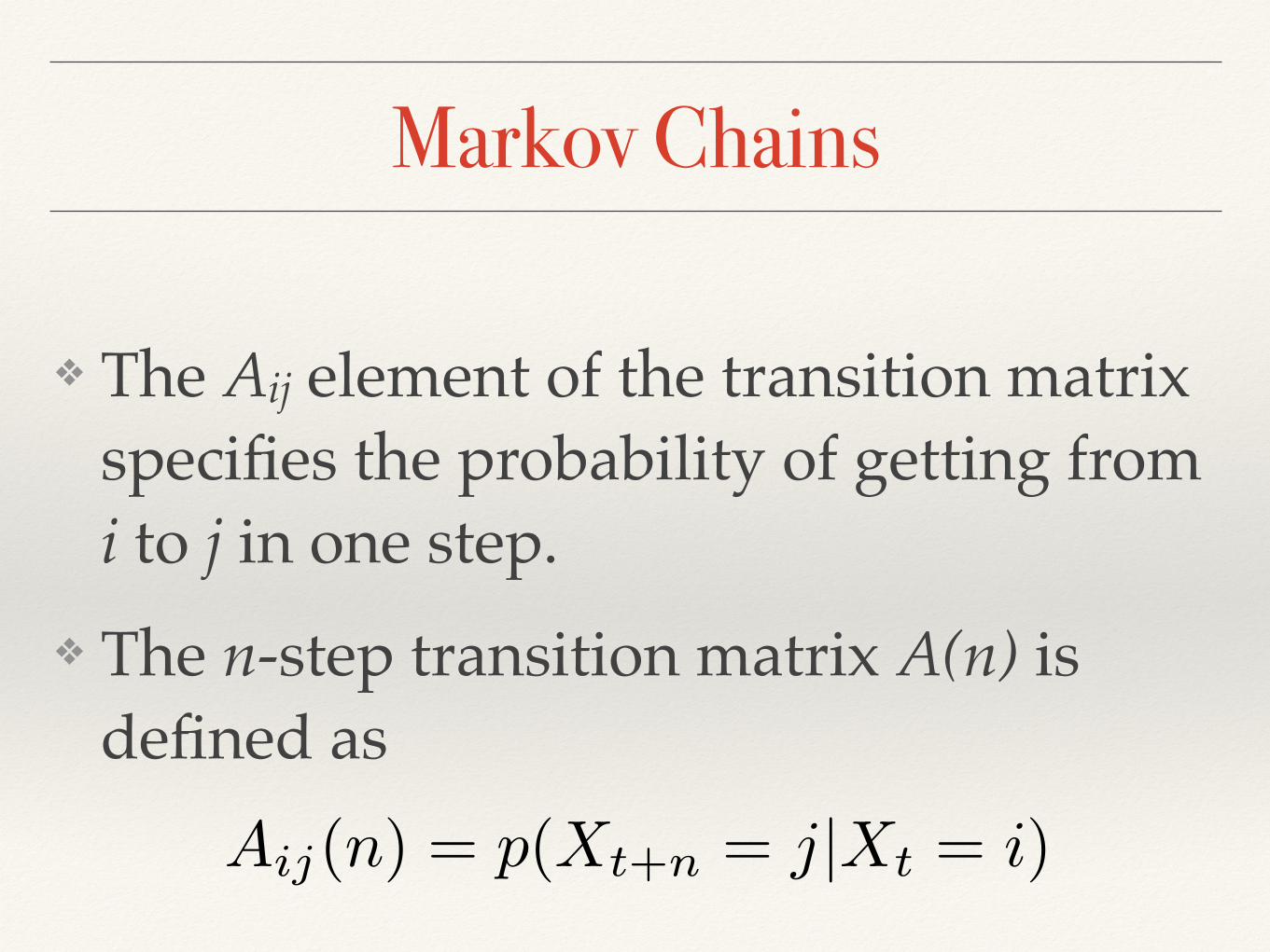
The Aij element of the transition matrix specifies the probability of getting from i to j inone step. The n-step transition matrix A(n) is defined as

Aij(n) ! p(Xt+n = j|Xt = i) (17.4)

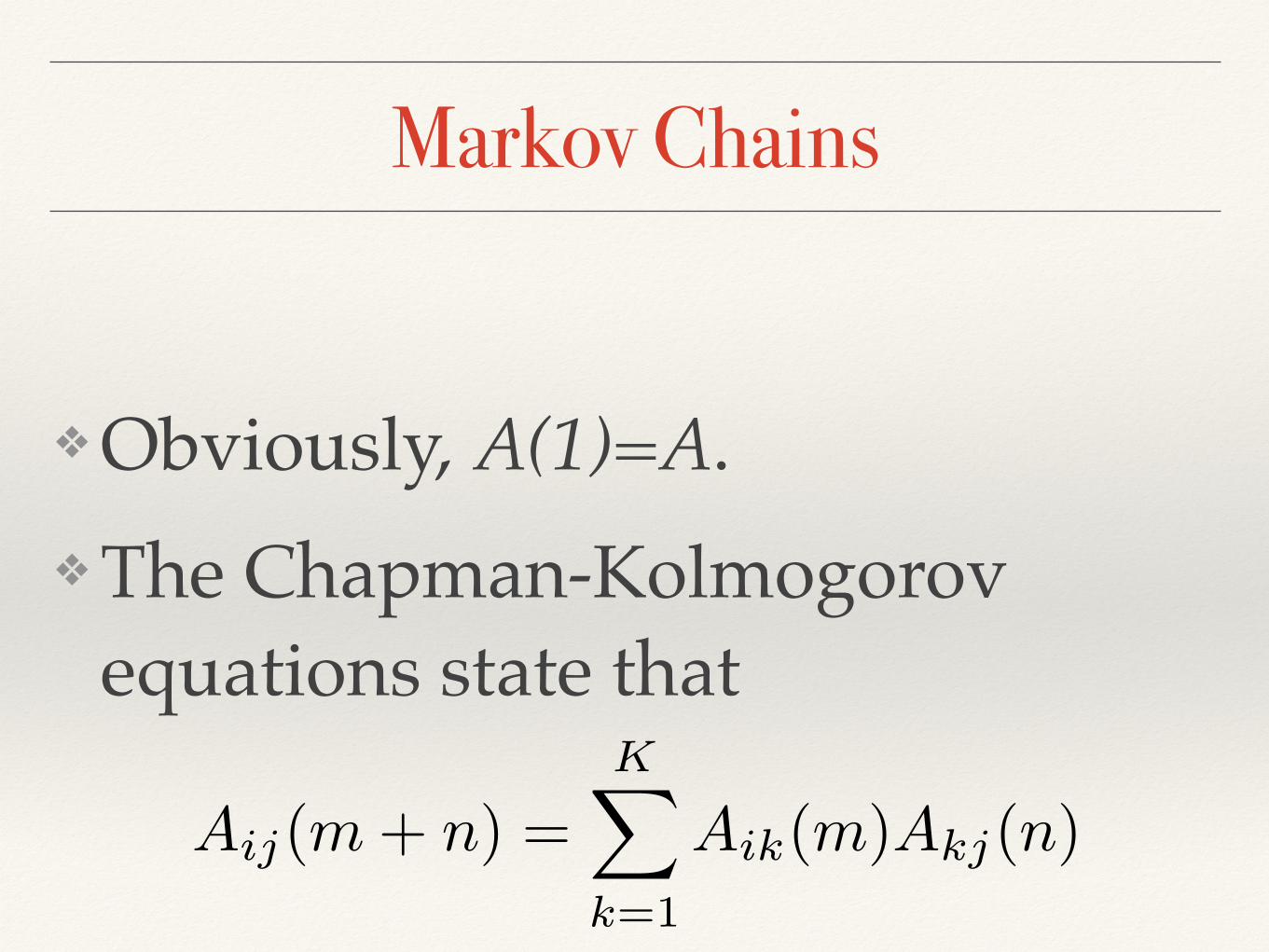
which is the probability of getting from i to j in exactly n steps. Obviously A(1) = A. TheChapman-Kolmogorov equations state that

Aij(m+ n) =K∑

k=1

Aik(m)Akj(n) (17.5)

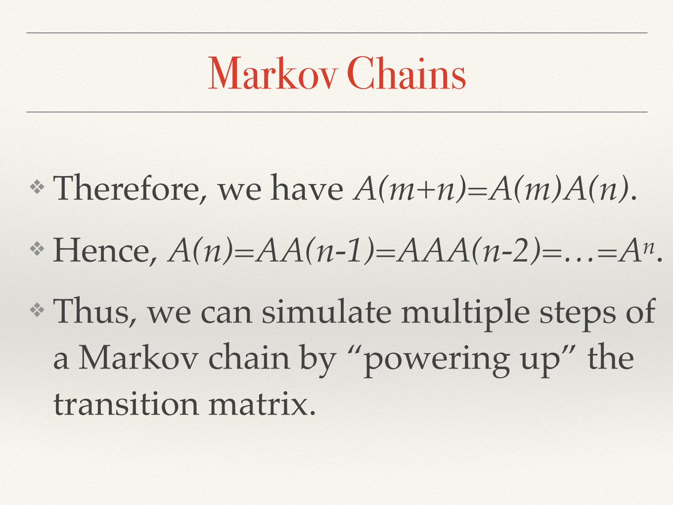
In words, the probability of getting from i to j in m+ n steps is just the probability of gettingfrom i to k in m steps, and then from k to j in n steps, summed up over all k. We can writethe above as a matrix multiplication

A(m+ n) = A(m)A(n) (17.6)

Hence

A(n) = A A(n− 1) = A A A(n− 2) = · · · = An (17.7)

Thus we can simulate multiple steps of a Markov chain by “powering up” the transition matrix.

590 Chapter 17. Markov and hidden Markov models

1 2

α

β

1− α 1− β

(a)

1 2 3

A12 A23

A11 A22 A33

(b)

Figure 17.1 State transition diagrams for some simple Markov chains. Left: a 2-state chain. Right: a3-state left-to-right chain.

A stationary, finite-state Markov chain is equivalent to a stochastic automaton. It is commonto visualize such automata by drawing a directed graph, where nodes represent states and arrowsrepresent legal transitions, i.e., non-zero elements of A. This is known as a state transitiondiagram. The weights associated with the arcs are the probabilities. For example, the following2-state chain

A =

(1− α αβ 1− β

)(17.2)

is illustrated in Figure 17.1(left). The following 3-state chain

A =

⎛

⎝A11 A12 00 A22 A23

0 0 1

⎞

⎠ (17.3)

is illustrated in Figure 17.1(right). This is called a left-to-right transition matrix, and is com-monly used in speech recognition (Section 17.6.2).

The Aij element of the transition matrix specifies the probability of getting from i to j inone step. The n-step transition matrix A(n) is defined as

Aij(n) ! p(Xt+n = j|Xt = i) (17.4)

which is the probability of getting from i to j in exactly n steps. Obviously A(1) = A. TheChapman-Kolmogorov equations state that

Aij(m+ n) =K∑

k=1

Aik(m)Akj(n) (17.5)

In words, the probability of getting from i to j in m+ n steps is just the probability of gettingfrom i to k in m steps, and then from k to j in n steps, summed up over all k. We can writethe above as a matrix multiplication

A(m+ n) = A(m)A(n) (17.6)

Hence

A(n) = A A(n− 1) = A A A(n− 2) = · · · = An (17.7)

Thus we can simulate multiple steps of a Markov chain by “powering up” the transition matrix.

Markov Chains

❖ The Aij element of the transition matrix specifies the probability of getting from i to j in one step.

❖ The n-step transition matrix A(n) is defined as

Aij(n) = p(Xt+n = j|Xt = i)

Markov Chains

❖ Obviously, A(1)=A. ❖ The Chapman-Kolmogorov

equations state that

Aij(m+ n) =KX

k=1

Aik(m)Akj(n)

Markov Chains

❖ Therefore, we have A(m+n)=A(m)A(n).❖ Hence, A(n)=AA(n-1)=AAA(n-2)=…=An.❖ Thus, we can simulate multiple steps of

a Markov chain by “powering up” the transition matrix.

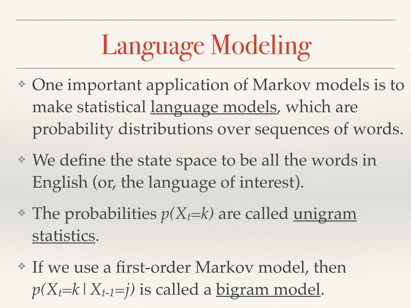
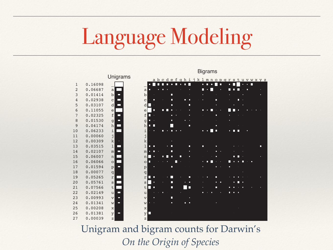
Language Modeling❖ One important application of Markov models is to

make statistical language models, which are probability distributions over sequences of words.

❖ We define the state space to be all the words in English (or, the language of interest).

❖ The probabilities p(Xt=k) are called unigram statistics.

❖ If we use a first-order Markov model, then p(Xt=k|Xt-1=j) is called a bigram model.

Language Modeling592 Chapter 17. Markov and hidden Markov models

1 0.16098 _ 2 0.06687 a 3 0.01414 b 4 0.02938 c 5 0.03107 d 6 0.11055 e 7 0.02325 f 8 0.01530 g 9 0.04174 h10 0.06233 i11 0.00060 j12 0.00309 k13 0.03515 l14 0.02107 m15 0.06007 n16 0.06066 o17 0.01594 p18 0.00077 q19 0.05265 r20 0.05761 s21 0.07566 t22 0.02149 u23 0.00993 v24 0.01341 w25 0.00208 x26 0.01381 y27 0.00039 z

Unigrams _ a b c d e f g h i j k l m n o p q r s t u v w x y z_abcdefghijklmnopqrstuvwxyz

Bigrams

Figure 17.2 Unigram and bigram counts from Darwin’s On The Origin Of Species. The 2D picture on theright is a Hinton diagram of the joint distribution. The size of the white squares is proportional to thevalue of the entry in the corresponding vector/ matrix. Based on (MacKay 2003, p22). Figure generated byngramPlot.

17.2.2.1 MLE for Markov language models

We now discuss a simple way to estimate the transition matrix from training data. The proba-bility of any particular sequence of length T is given by

p(x1:T |θ) = π(x1)A(x1, x2 ) . . . A(xT−1, xT ) (17.8)

=K!

j=1

(πj)I(x1=j)

T!

t=2

K!

j=1

K!

k=1

(Ajk)I(xt=k,xt−1=j) (17.9)

Hence the log-likelihood of a set of sequences D = (x1, . . . ,xN ), where xi = (xi1, . . . , xi,Ti)is a sequence of length Ti, is given by

logp(D|θ) =N"

i=1

logp(xi|θ) ="

j

N1j logπj +

"

j

"

k

Njk logAjk (17.10)

where we define the following counts:

N1j !

N"

i=1

I(xi1 = j), Njk !N"

i=1

Ti−1"

t=1

I(xi,t = j, xi,t+1 = k) (17.11)

Unigram and bigram counts for Darwin’s On the Origin of Species

Parameter Estimation for Markov Chains

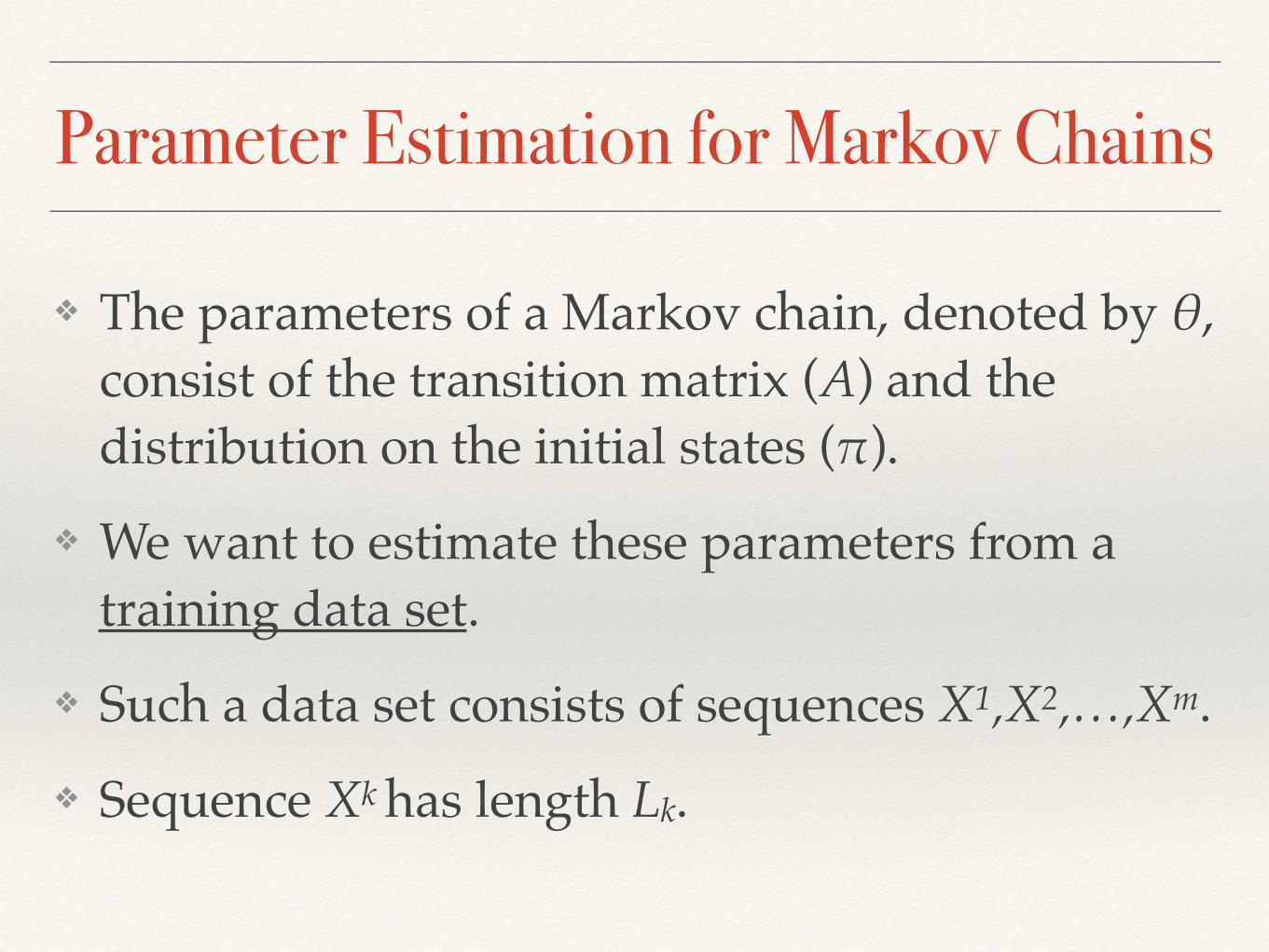
❖ The parameters of a Markov chain, denoted by θ, consist of the transition matrix (A) and the distribution on the initial states (π).

❖ We want to estimate these parameters from a training data set.

❖ Such a data set consists of sequences X1,X2,…,Xm. ❖ Sequence Xk has length Lk.


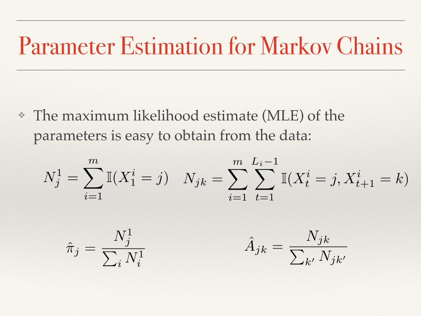
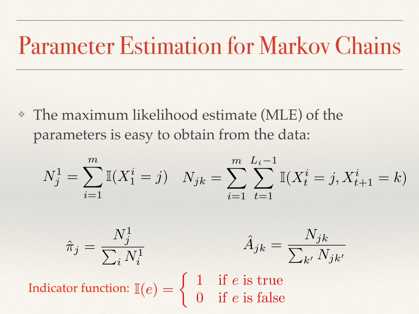
❖ The maximum likelihood estimate (MLE) of the parameters is easy to obtain from the data:

N1j =

mX

i=1

I(Xi1 = j) Njk =

mX

i=1

Li�1X

t=1

I(Xit = j,Xi

t+1 = k)

⇡j =N1

jPi N

1i

Ajk =NjkPk0 Njk0


❖ The maximum likelihood estimate (MLE) of the parameters is easy to obtain from the data:

N1j =

mX

i=1

I(Xi1 = j) Njk =

mX

i=1

Li�1X

t=1

I(Xit = j,Xi

t+1 = k)

⇡j =N1

jPi N

1i

Ajk =NjkPk0 Njk0

I(e) =⇢

1 if e is true0 if e is false

Indicator function:


❖ It is very important to handle zero counts properly (this is called smoothing).

Hidden Markov Models

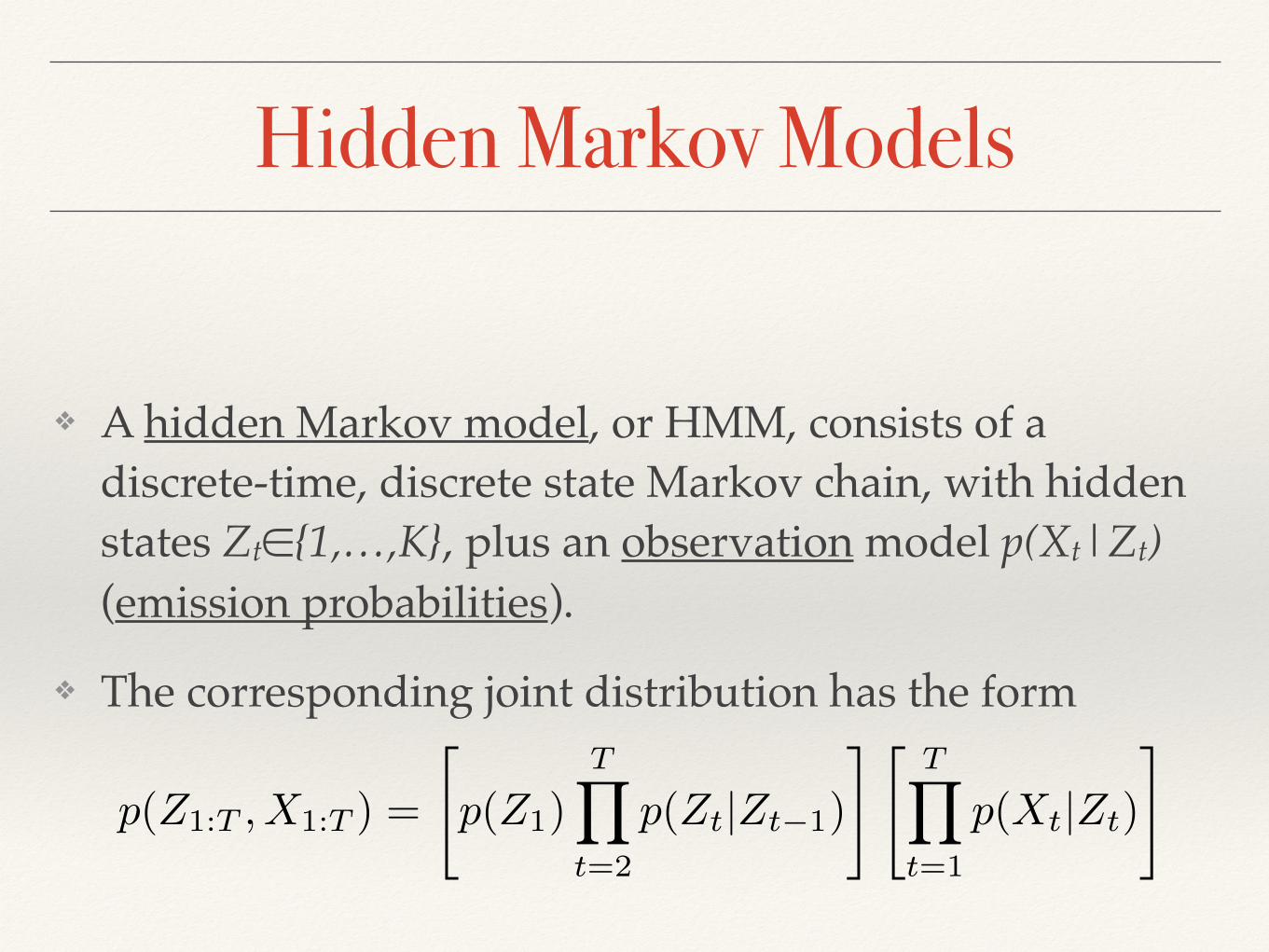
❖ A hidden Markov model, or HMM, consists of a discrete-time, discrete state Markov chain, with hidden states Zt∈{1,…,K}, plus an observation model p(Xt|Zt) (emission probabilities).

❖ The corresponding joint distribution has the form

p(Z1:T , X1:T ) =

"p(Z1)

TY

t=2

p(Zt|Zt�1)

#"TY

t=1

p(Xt|Zt)

#


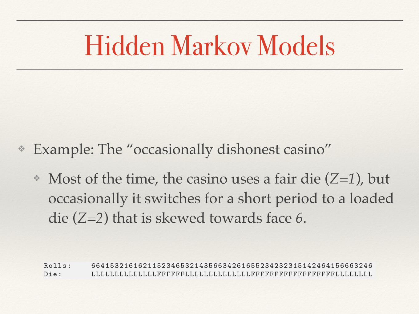
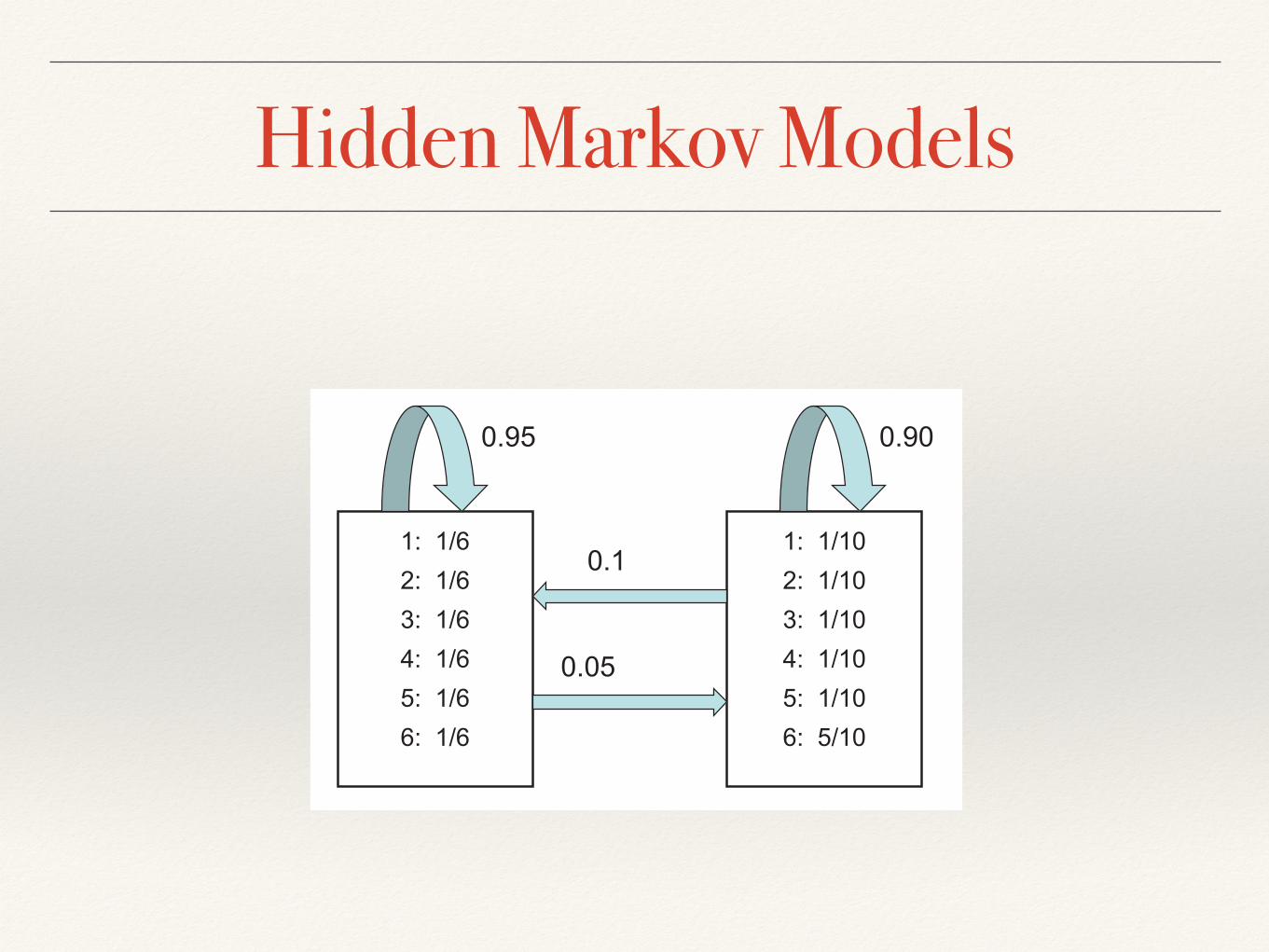
❖ Example: The “occasionally dishonest casino”

❖ Most of the time, the casino uses a fair die (Z=1), but occasionally it switches for a short period to a loaded die (Z=2) that is skewed towards face 6.


❖ Example: The “occasionally dishonest casino”

❖ Most of the time, the casino uses a fair die (Z=1), but occasionally it switches for a short period to a loaded die (Z=2) that is skewed towards face 6.

606 Chapter 17. Markov and hidden Markov models

related tasks.• Gene finding. Here xt represents the DNA nucleotides (A,C,G,T), and zt represents whether

we are inside a gene-coding region or not. See e.g., (Schweikerta et al. 2009) for details.• Protein sequence alignment. Here xt represents an amino acid, and zt represents whether

this matches the latent consensus sequence at this location. This model is called a profileHMM and is illustrated in Figure 17.8. The HMM has 3 states, called match, insert and delete.If zt is a match state, then xt is equal to the t’th value of the consensus. If zt is an insertstate, then xt is generated from a uniform distribution that is unrelated to the consensussequence. If zt is a delete state, then xt = −. In this way, we can generate noisy copies ofthe consensus sequence of different lengths. In Figure 17.8(a), the consensus is “AGC”, andwe see various versions of this below. A path through the state transition diagram, shownin Figure 17.8(b), specifies how to align a sequence to the consensus, e.g., for the gnat, themost probable path is D,D, I, I, I,M . This means we delete the A and G parts of theconsensus sequence, we insert 3 A’s, and then we match the final C. We can estimate themodel parameters by counting the number of such transitions, and the number of emissionsfrom each kind of state, as shown in Figure 17.8(c). See Section 17.5 for more information ontraining an HMM, and (Durbin et al. 1998) for details on profile HMMs.

Note that for some of these tasks, conditional random fields, which are essentially discrimi-native versions of HMMs, may be more suitable; see Chapter 19 for details.

17.4 Inference in HMMs

We now discuss how to infer the hidden state sequence of an HMM, assuming the parametersare known. Exactly the same algorithms apply to other chain-structured graphical models, suchas chain CRFs (see Section 19.6.1). In Chapter 20, we generalize these methods to arbitrarygraphs. And in Section 17.5.2, we show how we can use the output of inference in the contextof parameter estimation.

17.4.1 Types of inference problems for temporal models

There are several different kinds of inferential tasks for an HMM (and SSM in general). Toillustrate the differences, we will consider an example called the occasionally dishonest casino,from (Durbin et al. 1998). In this model, xt ∈ {1, 2, . . . , 6} represents which dice face showsup, and zt represents the identity of the dice that is being used. Most of the time the casinouses a fair dice, z = 1, but occasionally it switches to a loaded dice, z = 2, for a short period.If z = 1 the observation distribution is a uniform multinoulli over the symbols {1, . . . , 6}. Ifz = 2, the observation distribution is skewed towards face 6 (see Figure 17.9). If we sample fromthis model, we may observe data such as the following:

Listing 17.1 Example output of casinoDemoRolls: 664153216162115234653214356634261655234232315142464156663246Die: LLLLLLLLLLLLLLFFFFFFLLLLLLLLLLLLLLFFFFFFFFFFFFFFFFFFLLLLLLLL

Here “rolls” refers to the observed symbol and “die” refers to the hidden state (L is loaded andF is fair). Thus we see that the model generates a sequence of symbols, but the statistics of the

Hidden Markov Models17.4. Inference in HMMs 607

��

��

��

��

��

Figure 17.9 An HMM for the occasionally dishonest casino. The blue arrows visualize the state transitiondiagram A. Based on (Durbin et al. 1998, p54).

0 50 100 150 200 250 3000

0.5

1

roll number

p(loaded)

filtered

(a)

0 50 100 150 200 250 3000

0.5

1

roll number

p(loaded)

smoothed

(b)

0 50 100 150 200 250 3000

0.5

1

roll number

MA

P s

tate

(0=

fair,1

=lo

aded)

Viterbi

(c)

Figure 17.10 Inference in the dishonest casino. Vertical gray bars denote the samples that we generatedusing a loaded die. (a) Filtered estimate of probability of using a loaded dice. (b) Smoothed estimates. (c)MAP trajectory. Figure generated by casinoDemo.

distribution changes abruptly every now and then. In a typical application, we just see the rollsand want to infer which dice is being used. But there are different kinds of inference, which wesummarize below.

• Filtering means to compute the belief state p(zt|x1:t) online, or recursively, as the datastreams in. This is called “filtering” because it reduces the noise more than simply estimatingthe hidden state using just the current estimate, p(zt|xt). We will see below that we canperform filtering by simply applying Bayes rule in a sequential fashion. See Figure 17.10(a) foran example.

• Smoothing means to compute p(zt|x1:T ) offline, given all the evidence. See Figure 17.10(b)for an example. By conditioning on past and future data, our uncertainty will be significantlyreduced. To understand this intuitively, consider a detective trying to figure out who com-mitted a crime. As he moves through the crime scene, his uncertainty is high until he findsthe key clue; then he has an “aha” moment, his uncertainty is reduced, and all the previouslyconfusing observations are, in hindsight, easy to explain.


❖ Two important questions:

❖ How do we obtain the HMM?

❖ Given the observations, how do we find the hidden states that generated them?

Learning for HMMs

❖ The task of estimating the parameters (initial state distribution, transition, and emission probabilities)

❖ The more general case: Determining the set of states as well

❖ In practice, the states are often known

Learning for HMMs❖ Training from fully observed data:

❖ If we observe hidden state sequences, we can compute MLEs for the parameters, similar to the case of Markov chains

❖ Training when hidden state sequences are not observed is much harder:

❖ The Baum-Welch algorithm, which is an expectation-maximization (EM) algorithm, is used in this case (well beyond the scope of this course, though)

Computing the State Sequence

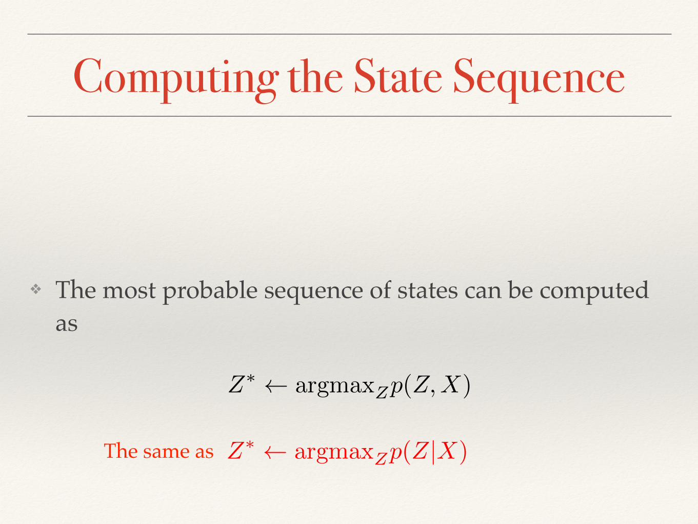
❖ The most probable sequence of states can be computed as

Z⇤ argmaxZp(Z,X)

Z⇤ argmaxZp(Z|X)The same as


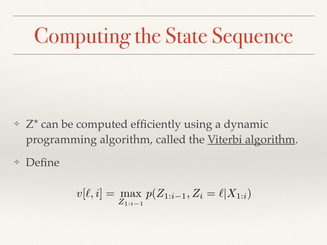
❖ Z* can be computed efficiently using a dynamic programming algorithm, called the Viterbi algorithm.

❖ Define

v[`, i] = maxZ1:i�1

p(Z1:i�1, Zi = `|X1:i)


COMP 182: Algorithmic Thinking Homework 6: Markov Models and POS Tagging

Start EndE 5 I

0.9 0.9

1.0 0.1 1.0 0.1

a=0.25b=0.25c=0.25d=0.25

a=0.05b=0.00c=0.95d=0.00

a=0.40b=0.10c=0.10d=0.40

Figure 1: HMM M .

(a) [4 pts] We are interested in the probability that a particle whose location at time t0 is node u

would be at node v at time tn. Represent the problem as a Markov chain (that is, describe thestates, initial state distribution, and transition matrix), and describe how to obtain the answerusing the Markov chain.

(b) [4 pts] We are interested in knowing the probability that a particle whose location at time t0 isany of the nodes in the graph (with uniform distribution) ends up at specific node v at time tn.Using the Markov chain representation from Part (a), how would you compute this probability?

3. [3 pts] The Viterbi algorithm (shown below) computes a path Z that optimizes p(Z,X) for a givensequence of observations X . Why is it a bad idea, instead, to compute a path Z that optimizes p(X|Z)?Illustrate your idea with a toy example of a 3-state HMM and sequence of words.

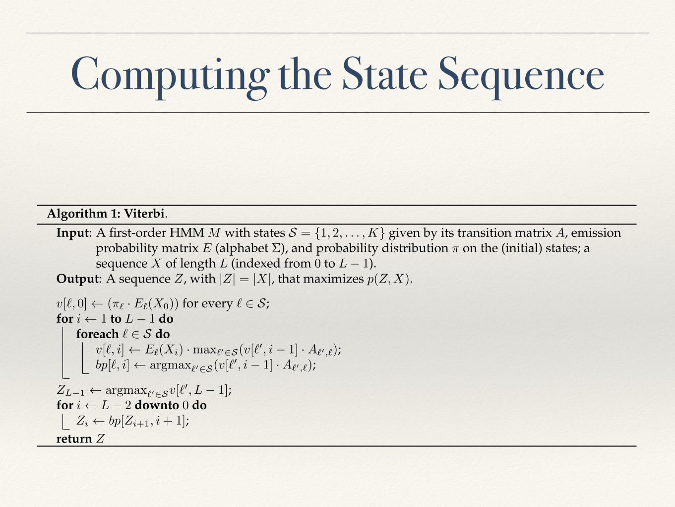
4. [7 pts] Algorithm Viterbi for first-order HMMs is given below. Give the pseudo-code of the Viterbialgorithm for second-order HMMs.

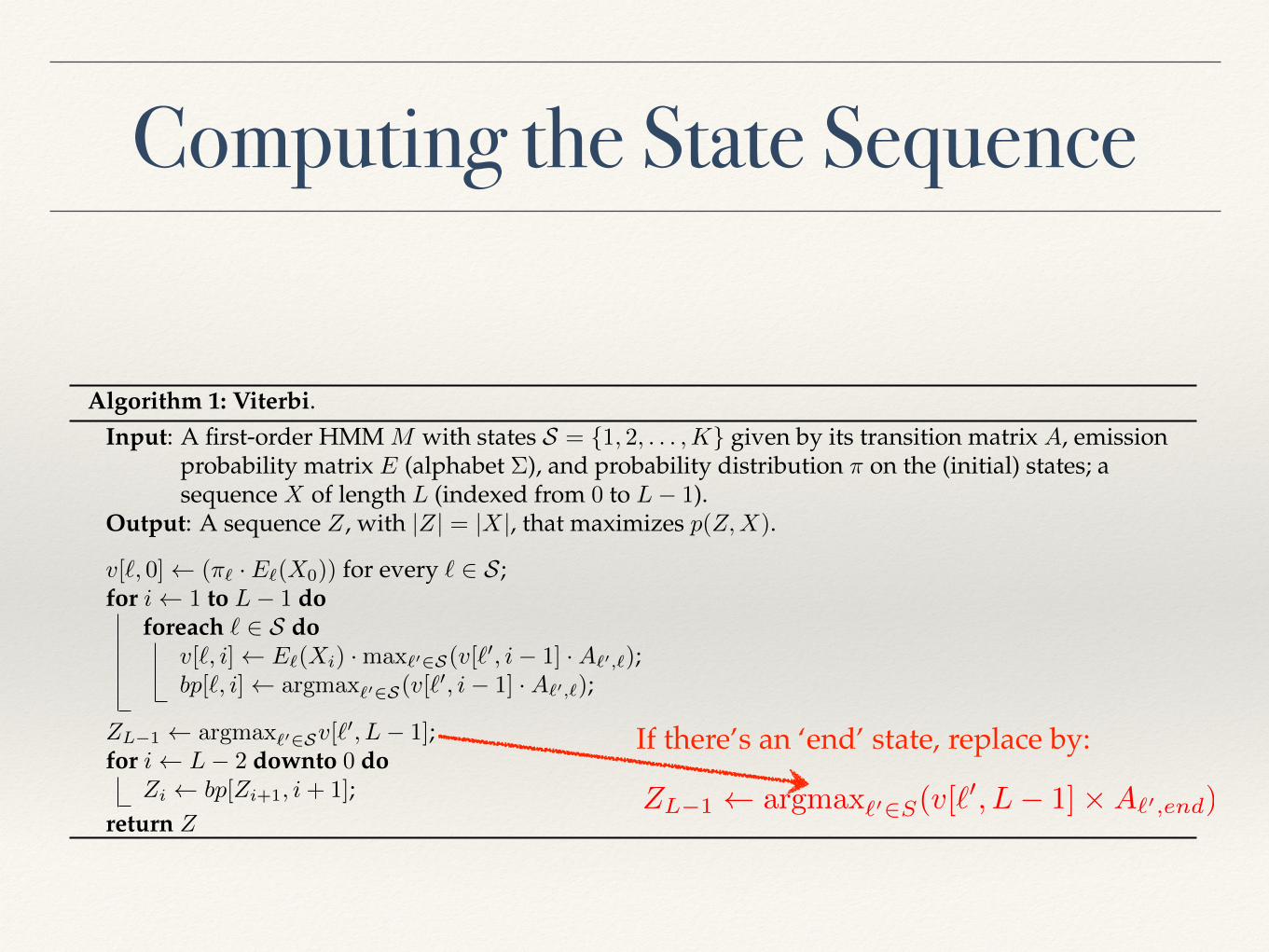
Algorithm 1: Viterbi.Input: A first-order HMM M with states S = {1, 2, . . . ,K} given by its transition matrix A, emission

probability matrix E (alphabet ⌃), and probability distribution ⇡ on the (initial) states; asequence X of length L (indexed from 0 to L� 1).

Output: A sequence Z, with |Z| = |X|, that maximizes p(Z,X).

v[`, 0] (⇡` · E`(X0)) for every ` 2 S ;for i 1 to L� 1 do

foreach ` 2 S dov[`, i] E`(Xi) ·max`02S(v[`0, i� 1] ·A`0,`);bp[`, i] argmax`02S(v[`

0, i� 1] ·A`0,`);

ZL�1 argmax`02Sv[`0, L� 1];

for i L� 2 downto 0 doZi bp[Zi+1, i+ 1];

return Z

5. [4 pts] Using big-O notation, what is the running time of the Viterbi algorithm for second-orderHMMs if the number of states is K and the length of the sequence of observations X is m.

3 Part-of-speech Tagging [56 pts]Part-of-speech tagging, or just tagging for short, is the process of assigning a part of speech or other syntacticclass marker to each word in a corpus. Examples of tags include ‘adjective,’ ‘noun,’ ‘adverb,’ etc. The input

2


COMP 182: Algorithmic Thinking Homework 6: Markov Models and POS Tagging

Start EndE 5 I

0.9 0.9

1.0 0.1 1.0 0.1

a=0.25b=0.25c=0.25d=0.25

a=0.05b=0.00c=0.95d=0.00

a=0.40b=0.10c=0.10d=0.40

Figure 1: HMM M .

(a) [4 pts] We are interested in the probability that a particle whose location at time t0 is node u

would be at node v at time tn. Represent the problem as a Markov chain (that is, describe thestates, initial state distribution, and transition matrix), and describe how to obtain the answerusing the Markov chain.

(b) [4 pts] We are interested in knowing the probability that a particle whose location at time t0 isany of the nodes in the graph (with uniform distribution) ends up at specific node v at time tn.Using the Markov chain representation from Part (a), how would you compute this probability?

3. [3 pts] The Viterbi algorithm (shown below) computes a path Z that optimizes p(Z,X) for a givensequence of observations X . Why is it a bad idea, instead, to compute a path Z that optimizes p(X|Z)?Illustrate your idea with a toy example of a 3-state HMM and sequence of words.

4. [7 pts] Algorithm Viterbi for first-order HMMs is given below. Give the pseudo-code of the Viterbialgorithm for second-order HMMs.

Algorithm 1: Viterbi.Input: A first-order HMM M with states S = {1, 2, . . . ,K} given by its transition matrix A, emission

probability matrix E (alphabet ⌃), and probability distribution ⇡ on the (initial) states; asequence X of length L (indexed from 0 to L� 1).

Output: A sequence Z, with |Z| = |X|, that maximizes p(Z,X).

v[`, 0] (⇡` · E`(X0)) for every ` 2 S ;for i 1 to L� 1 do

foreach ` 2 S dov[`, i] E`(Xi) ·max`02S(v[`0, i� 1] ·A`0,`);bp[`, i] argmax`02S(v[`

0, i� 1] ·A`0,`);

ZL�1 argmax`02Sv[`0, L� 1];

for i L� 2 downto 0 doZi bp[Zi+1, i+ 1];

return Z

5. [4 pts] Using big-O notation, what is the running time of the Viterbi algorithm for second-orderHMMs if the number of states is K and the length of the sequence of observations X is m.

3 Part-of-speech Tagging [56 pts]Part-of-speech tagging, or just tagging for short, is the process of assigning a part of speech or other syntacticclass marker to each word in a corpus. Examples of tags include ‘adjective,’ ‘noun,’ ‘adverb,’ etc. The input

2

ZL�1 argmax`02S(v[`0, L� 1]⇥A`0,end)

If there’s an ‘end’ state, replace by:

Questions?

COMP 182 Algorithmic Thinking Markov Chains andnakhleh/COMP182/MarkovChainsAndHMMs.pdfMarkov Chains...

Documents

Transcript of COMP 182 Algorithmic Thinking Markov Chains andnakhleh/COMP182/MarkovChainsAndHMMs.pdfMarkov Chains...