arX

iv:1

206.

2777

v1 [

hep-

th]

13 J

un 2

012

The geometry of antiferromagnetic spin chains

Dmitri Bykov∗

Nordita, Roslagstullsbacken 23, 106 91 Stockholm, Sweden

Steklov Mathematical Institute, Gubkina str. 8, 119991 Moscow, Russia

Abstract

We construct spin chains that describe relativisticσ-models in the continuum

limit, using symplectic geometry as a main tool. The target space can be an arbitrary

complex flag manifold, and we find universal expressions for the metric andθ-term.

NORDITA-2012-47

The true goal is not to reach the uttermost limits,

but to discover a completeness that knows no boundaries.

Rabindranath Tagore

1. Introduction

The application of coherent states in the physics of spin chains is a beautiful subject,

whose physics and mathematics sides are both extremely rich. The aim of this paper is

to apply the corresponding mathematical formalism to a description of long-range exci-

tations around antiferromagnetic vacua of particular spinchains withU(N) symmetry in

the quasiclassical (large spin) limit. The peculiarity of these spin chains is that the result-

ing continuum model is nothing but aσ-model with target space a flag manifold. More

concretely, we propose that theσ-model with target space U(N)U(n1)×···×U(nm) (

m∑

i=1ni = N) can be

obtained from a spin chain with the following Hamiltonian:

H =L∑

i=1

m−1∑

k=1

dk ~Si · ~Si+k, dk =

√

m− kk

(1)

In the above formula~Si represent the generators of a representation ofsuN, sitting at site

i. The representations atm consecutive sites can be described via Young diagrams that

consist of single columns of heightn1, · · · , nm, and a permutation of these sites generically

produces aσ-model with the same target space, but with a different metric andθ-term.

∗Emails: dbykov@nordita.org, dbykov@mi.ras.ru

1

The actual construction that produces the above result relies on methods from repre-

sentation theory and, even more importantly, symplectic geometry. Therefore we post-

pone the derivation of the results to Sections 4, 5 and begin this paper by giving an

overview of the mathematical formalism. One faces the necessity for this formalism as

soon as one embarks on the construction of a path integral representation for a spin chain,

which, in turn, is the most natural framework for the quasiclassical and continuum limits.

The construction of the spin chain path integral can be roughly separated in two stages:

the kinematical and dynamical parts. The kinematical part,which is the subject of Section

2, has to do with the description of the phase space of a singlespin — this is essentially

a part of representation theory, its aim being the description of coherent states in a given

representation of the global symmetry groupG. From the mathematical viewpoint, this is

an etude in the so-called Borel-Weil-Bott theorem, reviewed in Section 2.1 of the present

paper. SupposeG is a group of linear automorphisms of a vector spaceV. Quite generally,

the manifold of coherent states for any representation is a certain manifold of linear flags

in V, which can be viewed alternatively as an orbit ofG on the space of its coadjoint

representation. This statement allows one to make a connection to the method of orbits in

representation theory, and this is indeed necessary for theconstruction of the path integral.

It turns out that the kinetic part of the classical action forthe single spin is in fact given

by a particular symplectic form on the respective coadjointorbit. Therefore the solution

of the kinematical part of the problem may be viewed as a fruitof the Borel-Weil-Bott

theorem and the orbit method.

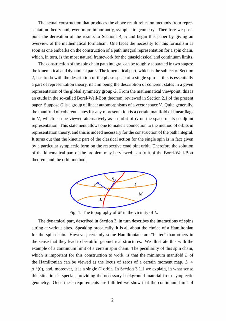
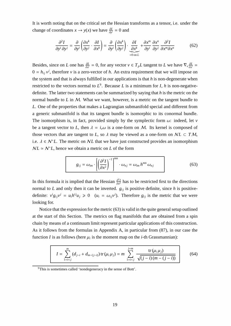
pq

LM

I

Fig. 1. The topography ofM in the vicinity of L.

The dynamical part, described in Section 3, in turn describes the interactions of spins

sitting at various sites. Speaking prosaically, it is all about the choice of a Hamiltonian

for the spin chain. However, certainly some Hamiltonians are “better” than others in

the sense that they lead to beautiful geometrical structures. We illustrate this with the

example of a continuum limit of a certain spin chain. The peculiarity of this spin chain,

which is important for this construction to work, is that theminimum manifoldL of

the Hamiltonian can be viewed as the locus of zeros of a certain moment map,L ≃µ−1(0), and, moreover, it is a singleG-orbit. In Section 3.1.1 we explain, in what sense

this situation is special, providing the necessary background material from symplectic

geometry. Once these requirements are fulfilled we show thatthe continuum limit of

2

this spin chain results in a two-dimensionalrelativistic sigma-model with target space

L. Moreover, the resulting Lagrangian of the sigma model can be described in a general

setup. It turns out that the metric onL can be obtained by a rather universal geometric

construction. The topologicalθ-term is in turn severely restricted by the translational

invariance of the spin chain and can be described in a simple way in terms of certain

canonical generators. One of the interesting consequencesof this result is that a simple

permutation of sites of the spin chain generically leads to adifferentθ-term. In a sense,

this is a way to physically realize the generators of the cohomology group H2(L,Zm)1!

According to the argument of Haldane [1], this term is related to the absence or presence

of a mass gap in the spin chain, and is therefore of crucial importance.

The appendices offer derivations of the results presented in Sections 4 and 5 ofthe

paper, as well as an example of integration over a flag manifold and an example of calcu-

lation of a quadratic Casimir using oscillator algebra.

This paper is in some sense a continuation of [2]. Some familiarity with that paper

will certainly be useful, in particular in order to understand the logic of our manipulations

with the spin chain Lagrangian in Sections 3.3, 4, 5 (although all calculations are given in

Appendix A). A large source of inspiration for this work is the paper of F.A.Berezin [3],

who was probably one of the first to introduce geometry into quantization in the sense

used in this paper, and the much more recent paper of E.Witten[4]. Important work

on the mathematical description of coherent states was doneby A.M.Perelomov, see [5].

Substantial work on the subject of Haldane continuum limitswas done by I.Affleck, see

[6] as an example.

2. Path integrals for spin chains

The goal of this Section is to review a general construction of path integral representa-

tions for spin chain partition functions. Roughly speaking, we are aiming at obtaining an

expression of the following sort:

Z ≡ tr (e−βHX) =∫

∏

i, t∈[0,1]

dµ(zi(t), zi(t)) exp (−S), where

zi ∈ CPN−1 and S = m

1∫

0

dt∑

i

(

izi zi

zi zi+ β

zi zi+1

zi zi

zi+1 zi

zi+1 zi+1

)

(2)

(3)

This formula is for a nearest neighbor spin-spin coupling described by the Hamiltonian

HX =∑

i

~Si · ~Si+1 with S U(N) symmetry;m is a positive integer indicating the represen-

tation at each site, i.e. it is them-th symmetric power of the fundamental. In what follows

1m refers to the number of factors in the denominator of the coset L = U(N)U(n1)×···×U(nm)

3

we will discuss various generalizations, both of the kinetic term (Sections 2.1, 2.2, 2.3)

and of the Hamiltonian (Section 3).

§ 2.1. The kinematical aspect. The Borel-Weil-Bott theorem.

SupposeH is a spin chain Hamiltonian with symmetry groupU(N). In this Section we

explain how one can write an expression for it in terms of the so-called coherent states.

In order to accomplish this task one first needs to find out whatthe coherent states are

for a given site of the spin chain. There is a very general theorem that gives an answer to

this question, which is usually attributed to Borel, Weil and Bott (BWB). It gives in fact

a complete geometric (and therefore beautiful) description of the whole representation

theory ofU(N) (it is also generalizable to other Lie groups, but we preferto focus here

on this simplest example). It goes as follows.

The assertion of the BWB theorem is that a finite-dimensionalrepresentation ofU(N)

with highest weight~λ can be modeled on the space of holomorphic sections of a holo-

morphic line bundle over a complete flag manifold

FN = U(N)/U(1)N. (4)

The line bundle is commonly denotedL~λ. Morally speaking, one can think of these sec-

tions as (not uniquely defined) functionsfi(z) on FN, which transform according to the

representationτ under the action ofG = U(N):

fi(g z) =dimτ∑

j=1

τ(g) ji f j(z) (5)

So how is the line bundleL~λ built? In order to understand this, first of all one has to know

the second cohomology of the flag manifold:

H2(FN,Z) = ZN−1, (6)

therefore there areN − 1 linearly independent 2-forms, that are the generators of H2(FN).

As a model for H2(F ) we will use the following. OnFN there areN standard (or tauto-

logical) line bundles,L1, · · · , LN, their sum being trivial:

N⊕i=1

Li = FN × CN . (7)

Their first Chern classes provide us withN closed 2-forms:Ωi = c1(Li), i = 1 · · ·N. Due

to the property (7) and the property of the first Chern classc1(E⊕ F) = c1(E)+ c1(F) one

4

sees thatΩi ’s are not independent but rather satisfy a relation

N∑

i=1

Ωi = 0 (8)

The 2-formsΩi, i = 1 · · · N, modulo the relation (8), generate H2(FN,Z).

There is another interesting take on the relation (8). It is related to Lagrangian sub-

manifolds, or Lagrangian embeddings, which are a leitmotifof the present paper, and we

feel it is time to introduce our main hero. What we want is a description ofFN, in which

the formsΩi arise naturally. The first thing to appreciate in this direction is the existence

of an embedding

i : FN → CPN−1 × · · · × CPN−1︸ ︷︷ ︸

N times

. (9)

A point m ∈ (CPN−1)×N is a set ofN lines through the origin inCN. Those points that

correspond toN orthogonallines are points ofFN — for this one should recall thatFN

may be thought of as a space ofN ordered orthogonal lines inCN. Let us consider the line

bundleO(1)i over eachCPN−1i factor. Thenωi ∼ c1(O(1)i) 2 can be taken as the Fubini-

Study form onCPN−1. The formsΩi introduced above can be built simply as pull-backs

of ωi toFN:

Ωi = i∗(ωi) (10)

With these ideas at hand, let us view (CPN−1)×N as a symplectic manifold with symplectic

form

ω =

N∑

i=1

ωi (11)

Our statement is that the embedding (9) is Lagrangian with respect to this symplectic

form, i.e.

ω|FN = 0. (12)

We postpone the proof to Section 3.2. Taking into account (10) and (12), the relation (8)

follows momentarily.

We have related the triviality of a certain line bundle overFN (N⊕i=1

Li = FN ×CN ) to

the fact thatFN is a Lagrangian submanifold of (CPN−1)N.

Now we are in a position to formulate the BWB result. To recallthe setup, we are

dealing with a representation ofU(N) with highest weightλ, and in the sequel we will

considerλ = (λ1, · · · , λN) to be the highest weight of the maximal torusU(1)N ⊂ U(N).

2∼means ‘in the same cohomology class’

5

The numbersλi are integers. Construct the following line bundle on (CPN−1)N:

Lλ = O1(λ1) ⊗ · · · ⊗ ON(λN) (13)

Pulling it back toFN, we get the line bundle of the BWB theorem:

Lλ = i∗(Lλ) (14)

The first Chern class of this bundle is equal to the following:

c1(Lλ) = i∗(Lλ) = i∗(N∑

i=1

λi ωi) =N∑

i=1

λi Ωi ≡ Ωλ (15)

The reason why we have been discussing this is that the pre-image ofc1(Lλ) under the

action of the external derivatived, i.e. the currentJ : dJ = c1(Lλ), is in the same

cohomology class with the kinetic term in the path integral.

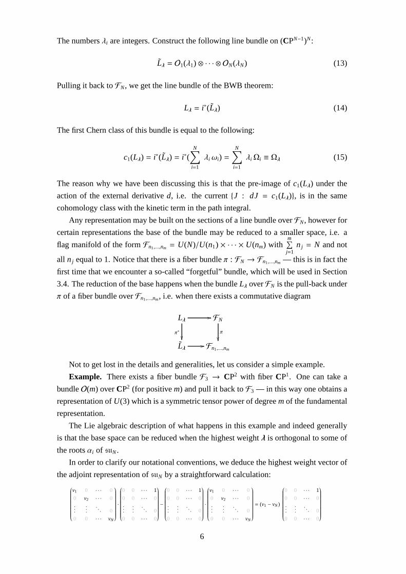
Any representation may be built on the sections of a line bundle overFN, however for

certain representations the base of the bundle may be reduced to a smaller space, i.e. a

flag manifold of the formFn1,...,nm = U(N)/U(n1) × · · · × U(nm) withm∑

j=1n j = N and not

all n j equal to 1. Notice that there is a fiber bundleπ : FN → Fn1,...,nm — this is in fact the

first time that we encounter a so-called “forgetful” bundle,which will be used in Section

3.4. The reduction of the base happens when the bundleLλ overFN is the pull-back under

π of a fiber bundle overFn1,...,nm, i.e. when there exists a commutative diagram

Lλ //

π∗

FN

π

Lλ // Fn1,...,nm

Not to get lost in the details and generalities, let us consider a simple example.

Example. There exists a fiber bundleF3 → CP2 with fiber CP1. One can take a

bundleO(m) overCP2 (for positivem) and pull it back toF3 — in this way one obtains a

representation ofU(3) which is a symmetric tensor power of degreemof the fundamental

representation.

The Lie algebraic description of what happens in this example and indeed generally

is that the base space can be reduced when the highest weightλ is orthogonal to some of

the rootsαi of suN.

In order to clarify our notational conventions, we deduce the highest weight vector of

the adjoint representation ofsuN by a straightforward calculation:

v1 0 · · · 0

0 v2 · · · 0...

.

.

.. . . 0

0 0 · · · vN

·

0 0 · · · 1

0 0 · · · 0...

.

.

.. . . 0

0 0 · · · 0

−

0 0 · · · 1

0 0 · · · 0...

.

.

.. . . 0

0 0 · · · 0

·

v1 0 · · · 0

0 v2 · · · 0...

.

.

.. . . 0

0 0 · · · vN

= (v1 − vN)

0 0 · · · 1

0 0 · · · 0...

.

.

.. . . 0

0 0 · · · 0

6

Hence, the highest weight vector of the adjoint representation looks as follows:

ρ = (1, 0, ..., 0,−1) (16)

The simple positive roots ofsuN can be found analogously and they have the following

form in our notations:

α1 = (1,−1, 0...0), α2 = (0, 1,−1, ...0), ... ,αN−1 = (0, 0, 0..., 1,−1) (17)

Therefore if for exampleλ ⊥ α1, it follows thatλ1 = λ2. It is convenient to portray

this diagrammatically: if the highest weightλ is orthogonal to a root, one colors the node

of the Dynkin diagram corresponding to this root [7].

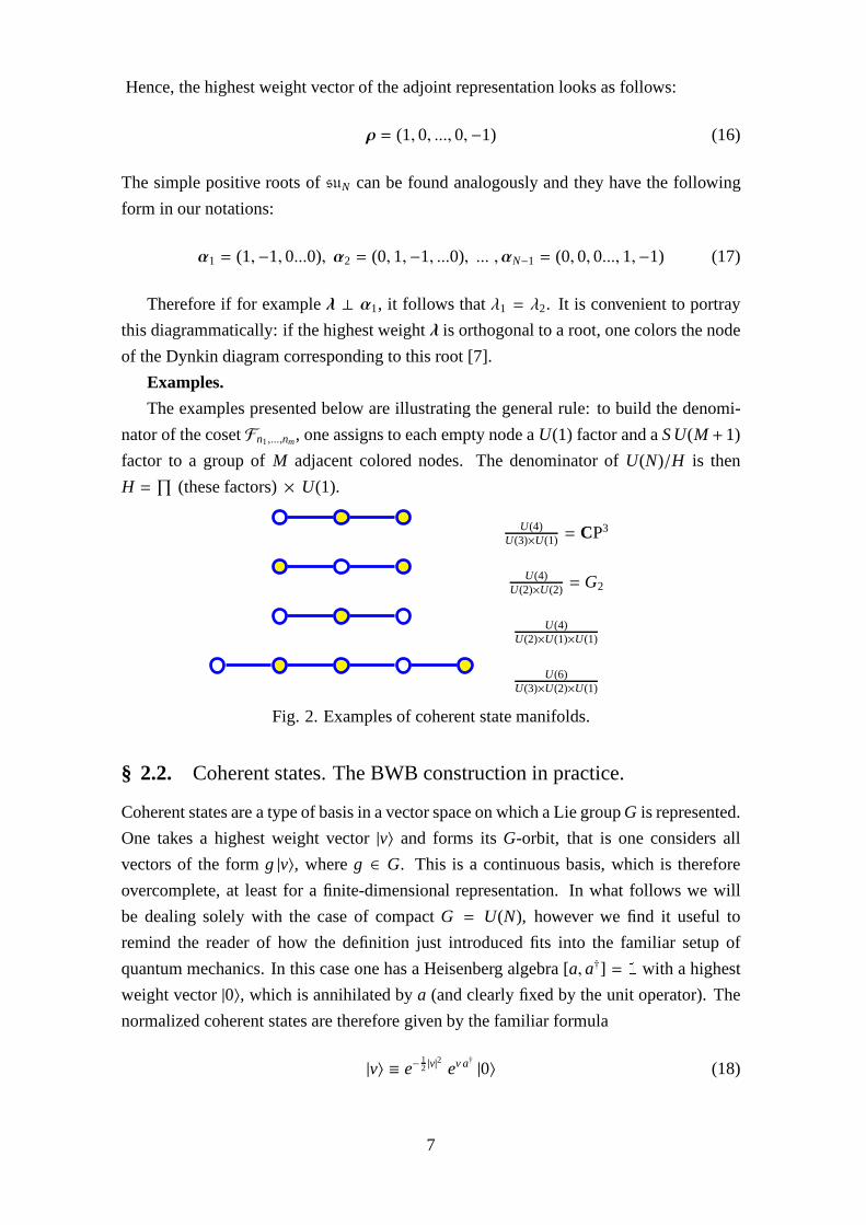
Examples.

The examples presented below are illustrating the general rule: to build the denomi-

nator of the cosetFn1,...,nm, one assigns to each empty node aU(1) factor and aS U(M +1)

factor to a group ofM adjacent colored nodes. The denominator ofU(N)/H is then

H =∏

(these factors) × U(1).

U(4)U(3)×U(1) = CP3

U(4)U(2)×U(2) = G2

U(4)U(2)×U(1)×U(1)

U(6)U(3)×U(2)×U(1)

Fig. 2. Examples of coherent state manifolds.

§ 2.2. Coherent states. The BWB construction in practice.

Coherent states are a type of basis in a vector space on which aLie groupG is represented.

One takes a highest weight vector|v〉 and forms itsG-orbit, that is one considers all

vectors of the formg |v〉, whereg ∈ G. This is a continuous basis, which is therefore

overcomplete, at least for a finite-dimensional representation. In what follows we will

be dealing solely with the case of compactG = U(N), however we find it useful to

remind the reader of how the definition just introduced fits into the familiar setup of

quantum mechanics. In this case one has a Heisenberg algebra[a, a†] = 1 with a highest

weight vector|0〉, which is annihilated bya (and clearly fixed by the unit operator). The

normalized coherent states are therefore given by the familiar formula

|v〉 ≡ e−12 |v|2 ev a† |0〉 (18)

7

§§ 2.2.1. The basis.

We start by building the bases in the relevant vector spaces using homogeneous polyno-

mials. Let us takeS U(3) as a first example. In this case the polynomials will be built out

of two sets of variables,a1, a2, a3 andb1, b2, b3.

a) a a a a Symmetric powers of the fundamental representation⇒ Symmet-

ric polynomials ina1, a2, a3 of degree 4.

b)a ab The adjoint representation⇒ Polynomials ina, b of the formai (a jbk−

akb j)

c)

a a ab bc The generalS U(N) case: 1) Assign to each row a lettera, b, c, · · · . 2)

For each column build antisymmetric combinations of the form∑

σ(−)σ aσ(i) bσ( j) cσ(k) dσ(l),

where the number of letters participating is equal to the height of the column. 3) Multiply

these antisymmetric combinations.

Remark 1. There are various linear relations among the polynomials built in the way

described inc). As a result, the representation is irreducible. For the exampleb) we could

take the following polynomials as a basis

Wi j = ai ǫ jmn am bn, i, j = 1 · · ·3 (19)

There is a single relation3∑

i=1Wii = 0, therefore the dimension of the vector space is 3×3−

1 = 8, as it should be.

Remark 2. From this construction it follows thatb enters only in antisymmetric

combinations witha, c enters in antisymmetric combinations withb anda, etc. Therefore

the basis constructed above does not change under the transformationb→ b+ r1a , c→c+ r2b+ r3a for arbitraryr1,2,3.

§§ 2.2.2. Coherent states from BWB.

In the case ofS U(N) the coherent states are polynomials of a particular sort. Having

the bases at hand, in order to build the coherent states all one needs to do is to pick a

particular state and form its orbit underS U(N). We will do it for the case of the three

Young diagrams shown above, and the general case will be clear from these examples.

a) Highest weight vectora41 leads toφv(a) = (v a)4, v ∈ CPN−1

b) Highest weight vectora1 · (a1b2 − a2b1) leads toφuvw(a, b) = (v a) · [(v a)(w b) − (w a)(v b)], w v = 0

c) Highest weight vectora1 · (a1b2−a2b1) · (a1b2c3−a1b3c2−a2b1c3−a3b2c1+a2b3c1+

8

a3b1c2) leads to

φuvw(a, b, c) = (v a) · [(v a)(w b) − (w a)(v b)] · (20)

·[(v a)(w b)(u c) − (v a)(u b)(w c) − (w a)(v b)(u c) −−(u a)(w b)(v c) + (w a)(u b)(v c) + (u a)(v b)(w c)]

with w v = u w = u v = 0.

In order to do calculations using these states one needs to know how to integrate over

a flag manifold. Appendix B provides an example — a proof of theParseval identity for

the systemb).

§§ 2.2.3. Relation to Schwinger-Wigner quantization.

In brief, Schwinger-Wigner quantization is a way of representing spin operators using

creation-annihilation operators (for a review see, for example, [8]).

Supposeτα are a set ofS U(N) generators in the fundamental representation. Introduce

N operatorsai and their conjugatesa†i with the canonical commutation relations

[ai, a†j ] = δi j . (21)

One can easily check that the operators

Sα = a†i ταi j a j, (22)

satisfy the commutation relations ofsu(N), andSα act irreducibly on the subspace of the

full Fock space specified by the condition

N∑

i=1

a†i ai = m, (23)

wherem is a positive integer representing the ‘number of particles’. For a givenm the rep-

resentation one obtains is them-th symmetric power of the fundamental representation.

What one should realize is that theai are, morally speaking, the homogeneous coordinates

zi onCPN−1. Indeed, if one imposes a partial gauge∑ |zi |2 = m in the path integral (2), the

kinetic term of the Lagrangian is simplyL0 = i∑

zi zi, therefore the canonical momen-

tumπi =∂L0∂zi= i zi, which leads to the algebrazi, zj = δi j , identical to (21). Needless to

say, this situation is general, and the correspondence holds for all representations.

To illustrate that this method is, nevertheless, not free from subtleties consider the

S U(3) adjoint representation of exampleb) from the previous section. To model this

9

representation on a subspace of the Fock space we build the operators

N1 = a†1a1 + a†2a2 + a†3a3, N2 = b†1b1 + b†2b2 + b†3b3 (24)

O1 = a†1b1 + a†2b2 + a†3b3 (25)

and we require the vectors|ψ〉 on which the representation is built to satisfy

N1|ψ〉 = 2 |ψ〉, N2|ψ〉 = |ψ〉, O1|ψ〉 = 0 (26)

The values ofN1 andN2 correspond to the number of boxes in the first and second rows

of the Young diagram. The expression for thesuN generators looks as follows

Sα = a†i ταi j a j + b†i τ

αi j b j , (27)

whereτα are the generators in the fundamental representation.

Notice that the classical condition ¯ab = 0 is translated toO1|ψ〉 = 0 with no counter-

partO†1|ψ〉 = 0. Indeed, the two equations would be incompatible, since [O1,O†1] = N1−N2

and (N1 − N2) |ψ〉 = |ψ〉 , 0. One might worry that this introduces a certain asymmetry

to the construction, however this asymmetry is the same one that is already present in the

Young diagram. In the general case we should introduceN creation operatorse†k for each

row k of the Young diagram (k = 1 corresponds to the first row, i.e. the longest one), and

impose the condition

Okm|ψ〉 ≡ e†k em |ψ〉 = 0 for k < m (28)

This is a compatible set of equations, since the operatorsOkm satisfy the algebra

[Okm,Onp] = δmnOkp − δkpOnm where k < m, n < p (29)

Okm may be thus thought of as the positive roots of the Lie algebrasuN.

Apart from its aesthetic appeal, this construction offers certain calculational benefits,

for instance the calculation of values of the Casimir operators on various representations

becomes a matter of simple oscillator algebra (for an example see Appendix C).

§ 2.3. The moment map for the action of loop rotations

In this Section we will look at the kinetic term in (3) from a slightly different angle. As

before, we will be assuming thatM is a symplectic manifold. Consider its loop space

LM, that is the space of all possible smooth embeddings of a circle S1 into M. A point of

the loop spaceγ ∈ LM is a loopγ(t) ∈ M : γ(1) = γ(0). A tangent vector toLM atγ is a

periodic vectorξ(t) ∈ Tγ(t)M : ξ(1) = ξ(0).

10

It is an important fact that one can, using the symplectic formΩ of M, define a sym-

plectic form Ω onLM. Indeed, supposeξ(t), η(t) are two tangent vectors toLM at γ.

Then the symplectic formΩ, evaluated on this pair of vectors, is:

Ω(ξ, η) =

1∫

0

dt Ω(ξ(t), η(t)) (30)

Now notice that onLM there is an action of the groupS of shifts along the loop. Clearly,

this group is isomorphic toU(1), since loops are circles. In more detail, the action of a

group elementgα ∈ S on a loopγ(t) is given by

gα γ(t) = γ(t + α) (31)

If we pick some local coordinatesxi on M, then the vector field, which generates this

action, can be written as follows3:

V =∫

dt xi(t)δ

δxi(t)(32)

This action also preserves the symplectic form (30). What isthe moment map associated

with this action? In order to answer this question we evaluateΩ onV to obtain a one-form:

Ω(•,V) =

1∫

0

dt Ω(δγ(t), γ(t)) (33)

or, in components,

Ω(•,V) =

1∫

0

dt δxi(t)Ωi j xj(t) (34)

We want to find such a functionµ on LM, whose variation under the contour change

δγ would produce the r.h.s. of (34). It turns out that such a function is nothing but the

“symplectic action”

µ(γ) =∫

Dγ

Ω, (35)

whereDγ is a disc inM havingγ as boundary. As it should, this expression, via the Stokes

theorem, only depends onγ — the boundary ofDγ. The symplectic action is of course

the same as the kinetic term in the classical action of the spin chain, for example the one

in (3).

3Note that the appearance of the functional derivative here is due to the fact thatLM is an infinite-dimensional space. Despite this, the groupS is one-dimensional.

11

§ 2.4. The action in supersymmetric form.

LetH = Sym(V⊗mfund) be the Hilbert space of a single spin. When the Hamiltonian is zero,

H = 0, the partition function of the spin may be written as follows (compare with 3):

Z = tr (1) = dimH =∫

∏

t∈[0,1]

dµ(z(t), z(t)) exp

−m

1∫

0

dt iz zz z

, (36)

wheredµ is the volume form onCPN−1.The volume form is proportional to the top power

of the Fubini-Study form. Once we have picked some local realcoordinatesx1... x2N−2 on

CPN−1, the Fubini-Study form may be written asω = ωi j dxi ∧ dxj. The volume form in

turn can be expressed asdµ = Pf(ω) dx1 ∧ dx2 ∧ ... ∧ dx2N, where Pf(ω) =√

detω. On

the other hand, there is an expression for the Pfaffian in terms of a Gaussian integral over

real fermions: Pf(ω) =∫ ∏

idψi eψi ωi j ψ j . Using this observation (36) may be rewritten

as follows:

Z =∫

∏

t∈[0,1]

dzi(t) ∧ zi(t)∏

t∈[0,1]

dψi(t) exp

−m

1∫

0

dt iz zz z

+ ψi(t) ωi j (t) ψ j(t)

(37)

The action in the exponent of this integral can be written in amanifestly supersymmetric

form, i.e. in a sort of superspace. Indeed, introduce two complex conjugate fermionic

coordinatesθ, θ and the following ‘superfields’:

Zi(t, θ) = zi(t) +1√

mθ ψi(t), i = 1 . . .N (38)

Zi(t, θ) = zi(t) −1√

mθ ψi(t) (39)

Then there is a remarkably simple expression for the action:

S = m

1∫

0

dt∫

dθ dθ K(Z, Z), where (40)

K(Z, Z) = ln

N∑

i=1

ZiZi

(41)

is the Kähler potential ofCPN−1.

3. The dynamical aspect.

In the sequel we will be elaborating on Hamiltonians whose minima may be described as

zero loci of moment maps. To this end we wish to remind the reader what the moment

12

map is and recall its main properties.

§ 3.1. Properties of the moment map.

Let M a symplectic manifold with the symplectic formΩ. Suppose there is an action of

a Lie groupG on M preserving the symplectic form, i.e.LXaΩ = 0, whereXa is a vector

field on M generating the action of a one-parametric subgroup ofG generated by the

elementa ∈ g andLY = d iY+ iYd is the Lie derivative. SinceΩ is closed by definition,

LXaΩ = 0 impliesd(iXaΩ) = 0, therefore ifM is simply connected (it will be the case in

all of the examples that we will consider), theniXaΩ = dµa, whereµa is a function onM

and, of course, it can also be regarded as a function ofa. In fact, since the vector fieldXa

depends ona linearly,µa is also a linear function of the Lie algebra elementa, therefore,

dropping the labela, i.e. considering alla’s at the same time, we may write thatµ ∈ g∗.Let us summarize the above facts in the following definition:the moment map is a map

µ : M → g∗ from a symplectic manifoldM to the dual of the Lie algebrag, possessing

the following two properties:

(1) it is G-equivariant, i.e.µ(g x) = Adg µ(x) ≡ gµ(x)g−1 for x ∈ M, g ∈ G.

(2) it is the generating function for Hamiltonians describing the action ofG on M, i.e.

dµa = iXaΩ for a ∈ g. (42)

We will mostly be dealing with a simple Lie groupG. Its Lie algebrag possess a

uniqueG-invariant (Killing) scalar product, and therefore using this scalar product we

will often forget the difference betweeng andg∗.

§§ 3.1.1. What if µ−1(0) is a single orbit?

One important property of the moment map is that its zero-value set, usually denoted by

µ−1(0), isG-invariant, that is ifµ(x) = 0 thenµ(g x) = 0: this is obvious from property

(1). Thereforeµ−1(0) is a collection ofG-orbits. Another fact, which will be cornerstone

for the construction that follows, is that the restriction of Ω to eachG-orbit in µ−1(0)

vanishes, i.e. eachG-orbit in µ−1(0) is an isotropic submanifold ofM. This follows from

(42) upon contraction with the vector fieldXb corresponding to a Lie algebra elementb:

iXbdµa ≡ ∂bµa = iXbiXaΩ = Ω(Xb,Xa) (43)

The left hand side is zero, since∂bµa is the derivative ofµa along µ−1(0). Therefore

Ω(Xb,Xa) = 0, which means that the symplectic form is zero on vectors tangent to the

orbit of G.

An isotropic submanifoldN ⊂ M can in principle have any dimension up to (and

inclusive of) dim M2 — in the latter caseN is called Lagrangian. There is a theorem which

13

explains in what case aG-orbit inµ−1(0) is Lagrangian: it is precisely whenµ−1(0) consists

of one G-orbit, or in other words whenµ−1(0) itself is aG-orbit4 5. Indeed, assume

thatµ−1(0) is aG-orbit. Therefore its tangent space is spanned by the vectors Xa, a ∈ gintroduced above. In general not all of them are linearly independent, so we pick a basis

X1, ...,Xd of linearly independent vectors (d = dim µ−1(0)). We can assign to itd one-

forms: λk = Ω(•,Xk). SinceXk are linearly independent,λk are linearly independent as

well (since the formΩ is nondegenerate). Therefore thed × D (D = dim M > d =

dimµ−1(0)) matrix

λ = λ1, λ2, . . . , ; λdT (44)

has rankd. On the other hand, ifv is a null-vector ofλ, it means thatΩ(v,Xk) = 0 = ∂vµak

for all k. This means that the equalityµ = 0 is preserved along vectorv, thereforev is

tangent toµ−1(0) and is therefore expressed as a linear combination of theXk. Since there

ared linearly independent vectorsXk, the nullity ofλ is d: null λ = d. By the rank-nullity

theorem

rankλ + null λ = D ⇒ 2d = D, (45)

which means thatµ−1(0) is Lagrangian.

The converse is also true, essentially by the same argument.SupposeL = µ−1(0) is

Lagrangian. Since a generic Hamiltonian vector for the Hamiltonian action of the group

G has the formwa = Ωi j ∂ jµa

∂∂xi for somea, we need to show that there is a sufficient

number of such independent vectors, more exactlyD2 . SinceΩ is nondegenerate, this

is equivalent to showing that the matrixλ = Ω(•,X1), · · · ,Ω(•,Xdimg)T has rankD2 .

Similarly to what we had before, the kernel of this matrix is composed of those vectors

u that leave the moment map unchanged and equal to zero:∂uµ = 0. Such vectors are

tangent toL, and therefore the nullity ofλ is equal to the dimension ofL, i.e. D2 . The

result follows once again from the rank-nullity theorem.

§ 3.2. Moment maps for flag manifolds.

In this paper we are talking solely about manifolds of linearflags in complex vector

spaces. Any such flag manifold is a quotient space (coset)F (n1, ..., nm) = U(N)/U(n1) ×· · · × U(nm). For the sake of practical calculations one usually writesa coset element as a

U(N)-valued functiong(x) using some coordinatesx. The action ofU(N), x→ x, is then

4For a proof different from the one presented here see [9].5This is only true with the condition that there areD − d linearly independent forms amongdµa

∣∣∣µ=0

,

whered = dimµ−1(0). Another way to put it is that the JacobianJ ≡ Dµa

Dxi

∣∣∣µ=0

has rankD − d. This is a

nondegeneracy condition, as can be seen from the following example:M = R2 = p, q, G = S O(2), µ =

p2 + q2 ⇒ dimµ−1(0) = 0, rankJ = 0. Hereµ−1(0) is a trivial orbit consisting of one point, but it iscertainly not a Lagrangian submanifold. The above requirement means, in plain language, that the tangentvectors toµ−1(0) are exactly those that annihilate the equationµ = 0 (i.e. they span the kernel ofdµa, whichis henced-dimensional).

14

presented as

g0 · g(x) = g(x) · h0, g0 ∈ U(N), h0 ∈ U(n1) × · · · × U(nm) . (46)

In order to write a moment map for this action we recall yet another way to think about

flag manifolds. Every spaceF (n1, ..., nm) may be regarded as a (co)-adjoint orbit (adjoint

and coadjoint representations are equivalent if there is a non-degenerate Killing metric,

as it happens forsuN). It means that, as a model ofF (n1, ..., nm), one can take an element

z ∈ suN and consider its orbit Orb(z) = g · z · g−1, g ∈ S U(N). One has to choose such

z that its stabilizer would beU(n1) × · · · × U(nm). In this case the moment map is simply

µ(g) = g · z · g−1 (47)

First of all, it has the right transformation propertyµ(g0 · g) = g0 µ(g) g−10 , which means

that µ possesses property (1). To verify property (2) one needs to write the symplectic

form onF in terms ofz andg . For this purpose we introduce the currentj = −g−1 · dg,

which obeys the flatness (Maurer-Cartan) equation

d j − j ∧ j = 0 (48)

In these terms the symplectic form is:

Ω = tr (z j∧ j) (49)

Due to the Maurer-Cartan equation, it is a closed form. We canassume thatz lies in

the Cartan subalgebra, since clearly every orbit Orb(z) intersects it. A simple calculation

reveals that forz in the Cartan subalgebra,z = diag(λ1, · · · , λN), the formΩ coincides

withΩ~λ introduced in 15. Suppose now thatva is a vector field onF corresponding to Lie

algebra elementTa. Then one can verify that

j(va) ≡ iva j = −g−1∇vag = −g−1 ddt

(

eTa t g) ∣∣∣t=0= −g−1Tag (50)

Using this, it is straightforward to check the defining property (2) of the moment map:

d(tr (µTa)) = d(tr (g z g−1 Ta)) = tr (z[ j, g−1Tag]) = iva tr (z j∧ j) = iva Ω (51)

§ 3.3. The Hamiltonian.

After this general discussion we come to the actual Hamiltonians. The Hamiltonians,

which we will consider, are built from interactions of the form κmnSmi Sn

j , wherei, j are

15

the sites of the spin chain, andκ is the Killing form6. We will assume that the spin chain

is translationally invariant, i.e. its Hamiltonian can be defined by shifting along the chain

of a Hamiltonian of a ‘unit cell’. The number of sites in the unit cell will depend on the

target space that we want to get in the sigma model. However, for unit cell of lengthm

the Hamiltonian is of the form7

H =L∑

i=1

m−1∑

k=1

dk~Si · ~Si+k,

where

dk =

√

m− kk

(52)

(53)

The expression fordk is derived in the Appendix A — it is the unique result if one insists

on the two-dimensional Lorenz invariance of the resulting sigma model.

In order to write the Hamiltonian in terms of the coherent states we note that for

expressions quadratic in the spins this can be done simply byreplacing the spins~Si by

the corresponding moment mapsµi ∈ suN. A fully honest calculation would involve the

construction of a path integral ‘from scratch’ — the interested reader is referred to [2] for

an idea of how this can be done. In any case, the Hamiltonian has the following form,

when written in coherent states:

H →L∑

i=1

l∑

k=1

dk tr (µi µi+k) (54)

We will assume that the manifold of coherent states is the GrassmannianGn ≡ U(N)U(n)×U(N−n)

for somen. It will be explained in the next Section why we can restrict to this case. The

moment map for the action ofS U(N) on a GrassmannianGn of n-planes has the form

µ =

n∑

k=1

zk ⊗ zk

zk zk− n

N1, (55)

where the vectorszk form an orthogonal basis in a givenn-plane: zm zn = δmn zm zm. It is not difficult to see that the Hamiltonian (54) is a sum of positive terms (apart

from some irrelevant constants), and the minimum is attained when all thez vectors at

neighboringm sites are orthogonal. This means that the correspondingni-dimensional

planes (i = 1 · · ·m) are orthogonal to each other (and together fill the vector spaceCN).

This configuration is precisely what we mean by theclassical antiferromagnetic vacuum.

6Such interaction is more easily visualizable when written in the form~Si · ~S j .

7The Hamiltonian considered in [2],H =L∑

i=1(Pi,i+1 +

12Pi,i+2), is a particular case whenm= 3.

16

§ 3.4. General equivariant Lagrangian embeddings:

forgetful fiber bundles.

In this section we discuss the geometric origins of the Lagrangian embeddings which we

have built using the moment map in the previous sections. Thequestion we want to an-

swer is: how big is the class of flag manifoldsM,N such that there existG-equivariant

Lagrangian embeddingsM →Lagr

N ? The answer that we will find is that for each flag

manifold M there is a canonical embedding into a product of symmetric spaces (Grass-

mannians)N.

Example. M = F3,N = (CP2)×3 .

We start once again from our basic example (already discussed in Section 2.1), as it

illustrates the general situation quite well. Recall thatF3 is interpreted geometrically as a

space of ordered 3-tuples of orthogonal three lines inC3. Therefore there exist three fiber

bundles, which associate with a given 3-tuple (v1, v2, v3) one of the three lines, eitherv1,

v2 or v3:

F3

π1②②②②

||②②②

π2

π3

""

CP2 CP2 CP2

The fiber= π−1i (pt) = CP1

Since each of these fiber bundles ‘forgets’ two lines out of three, they may be called

‘forgetful’ fiber bundles. They are explicitlyG = S U(3)-equivariant. The embedding

under consideration is seen to be the mapM → π1(M) × π2(M) × π3(M) = N. Since

we know this map is injective, or in other words that it does not send any two distinct

pointsa, b ∈ M to the same one inN, let us discuss what it means geometrically. If

it were not injective, that would mean thata andb lie simultaneously in all three fibers

f1 = π−11 (m), f2 = π−1

2 (n) and f3 = π−13 (p) of the corresponding fibrations, that is to

say (a, b) ∈ f1 ∩ f2 ∩ f3. Therefore we come to the conclusion that any three fibers

intersect in no more than one point. We can even be more specific: if m, n, p are not

mutually orthogonal, then the fibers of the corresponding fiber bundles do not intersect at

all, whereas if theyaremutually orthogonal, then the intersection consists of onepoint.

We now wish to generalize the above example to the case of a general flag manifold

Fn1, ··· ,nm = U(N)/U(n1) × · · · × U(nm). (56)

We can now buildmfiber bundles by forgetting the ‘fine structure’ of the flag andremem-

bering only one linear subspace (and its orthogonal) at a time:

Fn1, ··· ,nm =U(N)

U(n1)×···×U(nm)

π1♥♥♥♥

vv♥♥♥♥♥♥♥ ···

πmPP

PP

((PPP

PPPP

Gn1 · · · Gnm

whereGn =U(N)

U(n)×U(N−n) is the Grassmannian ofn-planes inCN.

17

The corresponding map

Fn1, ··· ,nm →m∏

j=1

Gnj (57)

is an embedding and, moreover, it is a Lagrangian embedding.First let us perform a

dimensionality check:

dimFn1, ··· ,nm = N2 −m∑

j=1

n2j , dimGn = N2 − n2 − (N − n)2 = 2(n · N − n2) (58)

⇒ dimm∏

j=1

Gnj = 2m∑

n=1

(n · N − n2) = 2

N2 −

m∑

n=1

n2

= 2 dimFn1, ··· ,nm (59)

Given the background accummulated to this moment, it is not difficult to show that the

embedding is Lagrangian. We need to construct a moment map for the diagonal action

of S U(N) on the product of Grassmannians and prove thatµ−1(0) is the flag manifold

under consideration. We have in fact already constructed the moment map for a single

Grassmannian in (55), so now we take a sum of those:

µ =

m∑

i=1

ni∑

k=1

zik ⊗ zik

zik zik

− 1 (60)

where we have used the relationm∑

i=1ni = N. One should recall that in this formula it is

implied thatzim zin = δmn. On the other hand, the setµ−1(0) is composed ofN-tuples

of orthogonalz-vectors. It follows that thez-vectors representing differentni-dimensional

planes inCN (i = 1 · · ·m) are mutually orthogonal. The set of such orthogonal subspaces

is precisely the flag manifoldFn1, ··· ,nm !

4. The metric.

On a general flag manifold, which is not necessarily a symmetric space, there may exist a

whole family ofS U(N)-invariant metrics8. The construction of continuum limits that we

are discussing in the present paper provides a particular representative from that family.

The aim of the present section is to give an intrinsic and universal expression for the

metric that arises in this context.

Let us recall the general setup, to which the remarks of the present section are gen-

erally applicable. One has a symplectic manifold (M, ω), a functionI onM and a La-

grangian submanifoldL ⊂ M, on whichI has a minimum. We can form the Hessian of

the functionI :

hi j =∂2I

∂xi∂xj(61)

8For an example of metrics on the complete flag manifoldU(N)/U(1)N see [2].

18

It is worth noting that on the critical set the Hessian transforms as a tensor, i.e. under the

change of coordinatesx→ y(x) we have∂I∂yi = 0 and

∂2I∂yi ∂yj

=∂

∂yi

(

∂xk

∂yj· ∂I∂xk

)

=∂

∂yi

(

∂xk

∂yj

)

· ∂I∂xk

︸︷︷︸

=0 onL

+∂xm

∂yi

∂xn

∂yj

∂2I∂xm∂xn

(62)

Besides, since onL one has∂I∂xi = 0, for any vectorv ∈ TpL tangent toL we have∇v

∂I∂xi =

0 = hi j vj, thereforev is a zero-vector ofh. An extra requirement that we will impose on

the system and that is always fulfilled in our applications isthath is non-degenerate when

restricted to the vectors normal toL9. BecauseL is a minimum forI , h is non-negative-

definite. The latter two statements can be summarized by saying thath is the metric on the

normal bundle toL inM. What we want, however, is a metric on the tangent bundle to

L. One of the properties that makes a Lagrangian submanifold special and different from

a generic submanifold is that its tangent bundle is isomorphic to its conormal bundle.

The isomorphism is, in fact, provided simply by the symplectic form ω: indeed, letv

be a tangent vector toL, thenλ = ivω is a one-form onM. Its kernel is composed of

those vectors that are tangent toL, soλ may be viewed as a one-form onNL ⊂ TM,

i.e. λ ∈ N∗L. The metric onNL that we have just constructed provides an isomorphism

NL ≃ N∗L, hence we obtain a metric onL of the form

gi j = ωim ·

(

∂2I∂x2

)−1

mn

· ωn j = ωim hmnωn j (63)

In this formula it is implied that the Hessian∂2I∂x2 has to be restricted first to the directions

normal toL and only then it can be inverted.gi j is positive definite, sinceh is positive-

definite: vigi j vj = uihi ju j > 0 (ui = ωi jvj). Thereforegi j is the metric that we were

looking for.

Notice that the expression for the metric (63) is valid in thequite general setup outlined

at the start of this Section. The metrics on flag manifolds that are obtained from a spin

chain by means of a continuum limit represent particular applications of this construction.

As it follows from the formulas in Appendix A, in particular from (87), in our case the

function I is as follows (hereµi is the moment map on thei-th Grassmannian):

I =m∑

1=i< j

(d j−i + dm−( j−i)) tr (µi µ j) = mj=m∑

1=i< j

tr (µi µ j)√

( j − i) (m− ( j − i))(64)

9This is sometimes called ‘nondegeneracy in the sense of Bott’.

19

5. The topological term.

Similarly to the case of the metric, one can build a universaland transparent expression

for the topological term that arises in the continuum limit of a spin chain. The idea is that

one can, once again, exploit the fact that there exists an embedding of the type (57) of a

general flag manifoldFn1, ··· ,nm = U(N)/U(n1) × · · · × U(nm) into a product of symmetric

spaces:

i : Fn1, ··· ,nm → Gn1 × ... ×Gnm, (65)

whereGn = U(N)/U(n) × U(N − n) is a Grassmannian (symmetric space). The most

natural fiber bundle to construct over such Grassmannian is the tautological bundle ofn-

planes that we will denote byOGn(1), analogously to the case ofCPN−1. The cohomology

ring of the original flag manifoldFn1, ··· ,nm may be built as a pull-back of the corresponding

cohomology ring of the Grassmannians. In particular, letrk = i∗(

c1(OGnk(1))

)

be the (pull-

back of the) first Chern class of the tautological bundle.rk satisfy a single relation

m∑

k=1

rk = 0 (66)

Then any element of H2(Fn1, ··· ,nm,Z) can be written as a linear combination with integer

coefficients of the pull-backs of these Chern classes. Finding theinteger coefficients that

describe the 2-formΩ arising in theθ-term is the goal of this Section.

The construction is, in fact, rather elementary. We start from a general expression for

the topological term:

mΩ =m∑

k=1

ak rk mod m, (67)

whereak are integers. The crucial requirement, which follows from the translational

invariance of the original Hamiltonian (52), is thatΩ should be invariant under a cyclic

permutation of the positions of the Grassmannians (indeed,their cyclic position simply

the way we ‘cut’ the spin chain into elementary cells, and this should not affect the result).

Denoting the permutation byΠ, we can formalize this requirement in the following way:

Π(mΩ) =m∑

k=1

ak+1 rk = mΩ mod m, (68)

When dealing with this equation, one should recall that there is a relation (66) on ther ’s,

therefore (68) may be rewritten as

m∑

k=1

ak+1 rk =

m∑

k=1

ak rk + nm∑

k=1

rk mod m, n ∈ Z (69)

20

or in other words

ak+1 − ak = n mod m (70)

Thereforeak = k·n mod m. In fact,n can be adjusted at will by taking symmetric powers

of representations at all nodes, so for the minimal choicen = 1 theθ-term can be written

as

Ω =1m

m∑

k=1

k · rk

(71)

As it should, the topological term of this form does not depend on thecyclic ordering of

the flag manifolds. Nevertheless, it follows from (71) that it certainly does depend on

their ordering (up to cyclic permutation). Therefore permuting the sites of the spin chain,

putting the representations in a different order, changes the topological term.

In particular, we come to the following interesting conclusion:

The basis of the cohomology group H2(Fn1,··· ,nm,Zm) can be obtained by permuting

the sites of the spin chain.

It is seen from (71) that the value ofθ is θ = 2πm . It also follows from the general

discussion of Section 2 that if one replaces the original representations at each site of the

spin chain by their symmetric tensor products of degreer, the value ofθ is multiplied by

r as a result.

6. Discussion.

In the present paper we had a two-fold goal: to give an overview of the geometrical

approach to representation theory (the Borel-Weil-Bott theorem) and coherent states and,

using them, to formulate two results concerning the long-wavelength limits of certain spin

chains. These infrared limits are two-dimensional sigma models, whose target space can

be an arbitrary flag manifold (though in the present paper we restrict ourselves to the case

of flags in complex vector spaces, i.e. the symmetry groupU(N)). We have shown that

for a flag manifold of our wish a spin chain can be built with a continuum limit described

by the sigma model with this flag manifold as its target space.The Hamiltonian of this

spin chain is given by (52), (53). From a mathematical point of view, our construction

relies on two facts:

1) The Hamiltonian is a function on a product of Grassmannians, which has a mini-

mum on a Lagrangian submanifold.

2) There exists a Lagrangian embedding of any flag manifold into a product of Grass-

mannians (65).

The submanifold, on which the Hamiltonian reaches a minimum, may be viewed as

the quasiclassical antiferromagnetic vacuum. It has to be Lagrangian, since it is only

21

in the vicinity of a Lagrangian submanifoldL that the original symplectic manifold (the

product of Grassmannians) looks as the cotangent bundle toL — the phase space of the

sigma model that we are building. From the more technical point of view, it is precisely

this circumstance that allows us to integrate over the momenta p, cotangent toL (see Fig.

1), and obtain an action quadratic in time derivatives (rather than linear in them, like the

original action).

The meaning of the second requirement is the following. The representations sitting

at the sites of the spin chain that we are considering are the ones appearing as spaces

of sections of holomorphic fiber bundles over Grassmannians. Therefore a product of

Grassmannians represents the union of several consecutivesites of the spin chain (the

elementary cell). The Hamiltonian, which is a function on this product of Grassmannians,

is then extended to the full spin chain by translational invariance. The fact thatanyflag

manifold can be embedded as a Lagrangian submanifold into a product of Grassmannians

simply means that for a given flag manifold we can always find a spin chain realizing its

geometry in the continuum limit.

The two main results of the paper are given by formulas (63) and (71). They provide

rather explicit expressions for the metric and topologicalterm of the resulting sigma mod-

els. We have found that in the situation when a functionI on a symplectic manifoldM has

a non-degenerate10 minimum on a Lagrangian submanifoldL ⊂ M, there is a canonical

metric onL that can be built using this data. It is given by formula (63).The functionI in

our case is given by 64.

As we have discussed in Section 5, the topological term can beobtained by a very

simple procedure. We form a linear combination of the first Chern classes of plane (tau-

tological) bundles over the Grassmannians into which our flag manifold is embedded (at

this point it is crucial to choose an ordering of the products) and then demand its invari-

ance under cyclic permutation of the Grassmannians in the product. This is a natural

requirement, since the cyclic permutation corresponds to ashift along the spin chain (or,

equivalently, a different partition of the spin chain into elementary cells), which should

not change the final result. There are two remarkable facts about the result (5). The first

one is that what enters the denominator in (5) ism— the number of Grassmannians in the

product, or the number ofU(ni) factors in the denominator of a fraction which describes

the flag manifold as a homogeneous space:U(N)U(n1)×···×U(nm) . This means that theθ-term be-

longs to the second cohomology group of the flag manifold withcoefficients inZm. It

would be interesting to understand if this implies any modm periodicity of the mass gap

in the spin chain. Another thing to notice is that in order to determine theθ-term we have

chosen an ordering of the Grassmannians in the product, or inother words the ordering

of sites in the spin chain. Therefore a different ordering gives a differentθ-term. One can

generate the cohomology group H2(F ,Zm) by permuting the sites of the spin chain!

10In the sense of Bott

22

Acknowledgments

I am grateful to Profs. S.Frolov, K.Zarembo for discussions. I am grateful to Prof.

E.Witten for his remarks to my talk at the conference “MathPhyz 2011”. I am especially

indebted to Prof. A.A.Slavnov for constant support and encouragement. My work was

supported in part by grants RFBR 11-01-00296-a, 11-01-12037-ofi-m-2011 and in part

by grant for the Support of Leading Scientific Schools of Russia NSh-4612.2012.1.

Appendices

A. Derivation of the metric and the θ-term.

In this Appendix we perform a complete calculation, which israther similar to the one

of [2], but more general. We have shown before that a generic flag manifold may be

embedded in a product of Grassmannians. Therefore we can restrict to the case when the

representations can be built from sections of fiber bundles over Grassmannians. We adopt

the simplest possible model for a Grassmannian. Consider the case of

Gn =U(N)

U(n) × U(N − n), (72)

We will represent it withN orthonormal complex vectorsuk, um un = δmn, where equiv-

alence relations are imposed on the sets of linesu1, · · · , un, un+1, · · · , uN. Each such

set represents a plane — the linear span of the correspondingvectors — therefore, for

example,u1, · · · , un ∼ u′1, · · · , u′n, if the two sets are related by aU(n) rotation of the

basis. The vectorsu1, · · · , un will enter all calculations only inU(n)-invariant combina-

tions. Callω the symplectic form onGn. The currentJ defined bydJ = ω can be built in

the following way

J = in∑

i=1

ui ui (73)

This is invariant with respect to theS U(n) gauge transformationsui → gi j u j, g ∈ S U(n),

since

J→ J + i ui uk︸︷︷︸

=δik

(g†g)ik = J, since tr (g† g) = 0 (74)

(For the caseg ∈ U(1) a total derivative is added toJ, and therefore the integratedJ-

current is invariant).

We will start from a Hamiltonian of the following general form:

H =∑

k

m−1∑

s=1

ds ~Sk · ~Sk+s . (75)

23

We therefore restrict to interactions of rangem − 1. Any consecutivem sites will be

therefore called a ‘unit cell’, or ‘elementary cell’.

Suppose the elementary cell is built ofl sites with a GrassmannianGni sitting at the

i-th site (i = 1 · · · l). One builds a moment map

µi =

ni∑

k=1

uk ⊗ uk −ni

N1. (76)

Then the spin-spin interaction of the form~Si · ~S j leads to the term

tr (µi µ j) ∼ 2∑

m<n

|u(i)m u( j)

n |2 + constant terms (77)

in the coherent state Hamiltonian. Therefore essentially the only difference from the case

of CPN−1 = G1 considered in detail in [2] is that now we have to sum over several similar

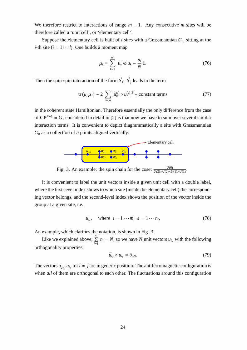
interaction terms. It is convenient to depict diagrammatically a site with Grassmannian

Gn as a collection ofn points aligned vertically.

u11 u21

u22

u31

u32

u41

Elementary cell

Fig. 3. An example: the spin chain for the coset U(6)U(2)×U(2)×U(1)×U(1).

It is convenient to label the unit vectors inside a given unitcell with a double label,

where the first-level index shows to which site (inside the elementary cell) the correspond-

ing vector belongs, and the second-level index shows the position of the vector inside the

group at a given site, i.e.

uiα , where i = 1 · · ·m, α = 1 · · ·ni , (78)

An example, which clarifies the notation, is shown in Fig. 3.

Like we explained above,m∑

i=1ni = N, so we haveN unit vectorsuiα with the following

orthogonality properties:

uiα uiβ = δαβ. (79)

The vectorsu jα , uiβ for i , j are in generic position. The antiferromagnetic configuration is

whenall of them are orthogonal to each other. The fluctuations aroundthis configuration

24

are conveniently constructed using the Gram-Schmidt (QR) decomposition. We set

z1 = u11, · · · zn1 = u1n1, (80)

zn1+1 = u21 +

n1∑

s=1

a21|1s u1s,

· · ·

znt+q = ut+1q +

t∑

m=1

nm∑

s=1

at+1q|ms ums, 1 6 q 6 nt+1

Summing only over the vectors from previous sites of the spinchain ensures that theziα , ziβ

are orthogonal11. In what follows we will assume thataiα| jβ = 0 for i < j. The formulas

written above are forz’s in the same elementary cell. In order to pass to a different cell

one has to assign an extra indexk in order to be able to differentiate between them. First

let us evaluate the interaction between two sites inside oneelementary cell:

i < j ⇒ |ziα zjβ |2 ∼ |a jβ |iα |2 (81)

The part of the Hamiltonian describing interactions insideblock k is as follows:

Hk =∑

i< j

d j−i

∑

α, β

·|akjβ |iα |

2 (82)

Now let us evaluate the interactions between two adjacent blocks,k − 1 andk. We note

that

⇒ |z(k−1)iα z(k)

jβ|2 ∼ |u(k−1)

iα u(k)

jβ+ ak

jβ|iα + ak−1iα | jβ |

2 ∼ |u(k)iα ∂xu

(k)jβ+ ak

jβ |iα + ak−1iα | jβ |

2, (83)

Given our choice of Hamiltonian of interaction rangem− 1, it is easy to show that for

ik−1 < jk the interaction is zero, i.e.d(ik−1, jk) = 0 for ik−1 < jk. Indeed, the distance

between these sites is thenjk + (N − ik−1) > N, whereas the interaction range ism− 1 6

N−1. Therefore the part of the Hamiltonian corresponding to inter-block interactions can

be thus written as

Hk−1,k =∑

i> j

dm−(i− j)

∑

α,β

|u(k)iα ∂xu

(k)jβ+ ak

iα | jβ |2 (84)

We have used the fact that the functiond(ik−1, jk) depends only on the distance between

the sitesik−1 and jk, which, as is easy to see, is the same asm− (i − j) (we are assuming

that i > j), i.e. d(ik−1, jk) = dm−(i− j).

11To first order inas. Generally, one has to writezn1+2 = u22 + νu21 +n1∑

s=1a22|1s u1s and impose the

orthogonality condition ¯zn1+1 zn1+2 = ν +n1∑

s=1a21|1s a22|1s = 0. This shows thatν is quadratic in thea’s and

therefore can be neglected in our approximation.

25

The full Hamiltonian has the following form

H =∑

k

∑

i< j, α, β

[

dm−( j−i) · |akiα | jβ |

2 + dm−( j−i) · |akiα| jβ − u(k)

jβ ∂xu

(k)iα|2]

= (85)

=∑

k

∑

i< j, α, β

[

(d j−i + dm−( j−i)) · |akiα | jβ |

2−

−dm−( j−i) · (akiα | jβ u(k)

jβ ∂xu

(k)iα+ ak

iα | jβ u(k)jβ ∂xu

(k)iα

) + dm−( j−i) |u(k)iα ∂xu

(k)jβ|2]

Now we need to write a corresponding expansion for the kinetic term:

L0 = i∑

k, i< j, α, β

(

akiα | jβ u(k)

jβ ∂tu

kiα − c.c.

)

(86)

Combining the above expressions we get the full Lagrangian in the form

L =∑

k

∑

i< j, α, β

[

(d j−i + dm−( j−i)) · |akiα | jβ |

2− (87)

−akiα | jβ (dm−( j−i) u(k)

jβ ∂xu

(k)iα+ i u(k)

jβ ∂tu

(k)iα

)−−ak

iα | jβ (dm−( j−i) u(k)jβ ∂xu

(k)iα− i u(k)

jβ ∂tu

(k)iα

)+

+dm−( j−i) |u(k)iα ∂xu

(k)jβ|2]

The last remaining step is to perform Gaussian integration over akiα | jβ . This is done using

the simple formula

A|w|2 + Bw+Cw = A(w+CA

)(w+BA

) − BCA

(88)

One obtains

L →∑

k

∑

i< j, α, β

[

dm−( j−i) |u(k)iα ∂xu

(k)jβ|2− (89)

− 1d j−i + dm−( j−i))

(dm−( j−i) u(k)jβ ∂xu

(k)iα+ i u(k)

jβ ∂tu

(k)iα

) ×

×(dm−( j−i) u(k)jβ ∂xu

(k)iα− i u(k)

jβ ∂tu

(k)iα

))]

We rewrite it in the form isolating the ‘metric’ part and theθ-term part:

L →∑

k

∑

i< j, α, β

[

−1d j−i + dm−( j−i)

(

|u(k)jβ ∂tu

(k)iα

)|2 − d j−idm−( j−i)|u(k)iα ∂xu

(k)jβ|2)

+ (90)

+dm−( j−i)

d j−i + dm−( j−i))

(

i (u(k)jβ ∂tu

(k)iα

) (u(k)jβ ∂xu

(k)iα

) − i (u(k)jβ ∂tu

(k)iα

)(u(k)jβ ∂xu

(k)iα

))]

26

As the first line shows, in order for the result to be Lorenz-invariant, we should require

dkdm−k = const.≡ D2 (independent ofk) (91)

In this case the metric on the flag manifold is described in terms of the matrix12

λk =D

dk + dm−k. (92)

Another requirement that we impose on our system is that theθ-term is a topological

invariant, in other words the second line of (90) should be a closed 2-form. This leads to

additional constraints on the coefficientsdl. We will get the following result:

dk =

√

m− kk

, λk =

√k (m− k)

m. (93)

Indeed, the second line of (90) can be thought of as a pull-back to the worldsheet of the

following form:

ω =∑

i< j

µ j−i ωi j with µk =dm−k

dk + dm−k, (94)

where

ωi j =∑

α,β

i u jβ duiα ∧ u jβ duiα . (95)

Introduce also the followingclosedforms

ωi =

m∑

j=1

ωi j . (96)

Note thatωi representsc1(OGni(1)). There is a single relation between these forms (since

ω ji = −ωi j )m∑

i=1

ωi = 0 (97)

We want to find suchµk’s for whichω is expressible as a linear combination ofωi ’s:

m∑

i=1

ai ωi = ω =∑

i< j

µ j−i ωi j (98)

One can see that this implies

µ j−i = a j − ai (99)

Since the l.h.s. depends only on the differencej − i, we find that

a j = j α + const., (100)

12We have rescaled the space coordinatex→ Dx in order to set the speed of light equal to 1.

27

whereα = µ1 and the constant is inessential, since its effect is to shift the formω by∑

ωi = 0. Therefore we set the constant to zero. From the explicit expression forµk it

follows thatµk + µm−k = 1, therefore

µk + µm−k = α k+ α (m− k) = αm= 1⇒ α =1m

(101)

In other words

ω =1m

m∑

j=1

j ω j , (102)

so we have arrived at the result announced in Section 5.

Using the definition ofµk, (94), and the relations 99 we get the following equations

µk =dm−k

dk + dm−k=

D2

d2k + D2

=km

(103)

Solving fordk, we obtain

dk = D

√

m− kk

(104)

which is the formula reported in (53), up to an inessential factor of D, which is simply

the normalization of the Hamiltonian. Clearly, thesedk satisfy the Lorenz invariance

condition (91). Our derivation is thus complete.

B. Integrating over the flag manifold F3

In the paper [2] we dealt rather closely with the case when themanifold of coherent states

is CPN−1. The reader might wonder, what changes arise in the general case — the one of

the flag manifold. To resolve the doubts we provide an example: namely, we prove the

completeness of the system of coherent states

φuvw(a, b) = (v a) · [(v a)(w b) − (w a)(v b)], w v = 0 (105)

in the vector spaceVadj of the adjoint representation ofsu3. According to (19) this space

is a subspace of the space of homogeneous polynomials in (a, b) if bidegree (2, 1). On the

space of polynomials of degreem in N variablesz1 · · · zN we will use the scalar product

〈 f | g〉 =∫ N∏

i=1

dzi dziĚf (z) g(z) e−|z|

2(106)

28

For the case at handN = 3, of course. We want to show that for any two states〈 f |, |g〉the following identity holds:

〈 f | g〉 =∫

dµF3(v,w, u)〈 f | φuvw〉 〈φuvw | g〉〈φuvw | φuvw〉

(107)

for some volume elementdµF3 on the flag manifold. Although the coherent stateφuvw

does not depend on the variableu (the third line in the flag), we still need to integrate

over it, since it is nontrivially entangled with the other coordinates by the measure. Note

that all multiplicative constants arising in the proof may be absorbed indµF3, therefore

we will not keep track of them. Using (106) one finds out that (107) is equivalent to the

following identity involving the coherent states only:

∫

dµF3(v,w, u)φuvw(a, b) Ěφuvw(c, d)〈φuvw | φuvw〉

= (c a)(

(c a) (d b) − (c b) (d a))

︸ ︷︷ ︸

≡Pr(a,b | c,d)

(108)

The reason for this is that the r.h.s. is the ‘kernel’ of the projection operator on the adjoint

representation:

∫

dc dc dd dd Pr(a, b | c, d) e−|c|2−|d|2 f (c, d) = f (a, b) for f ∈ Vadj (109)

The volume element onF3 may be written as follows (up to a constant):

dµF3(v,w, u) = dµCP2(u) dµCP2(v) dµCP2(w) δ(2)(w v) δ(2)(w u) δ(2)(v u) (110)

The most convenient way to deal with theCP2 volume element is to pull it back toC3,

using the tautological bundle. It can be done as follows:

dµCP2(u) = du1 ∧ du2 ∧ du3 ∧ du1 ∧ du2 ∧ du3 e−

3∑

i=1|ui |2

(111)

We are to integrate functions onCP2, i.e. functions onC3 invariant under a global

rescaling. Such functions do not depend on the ‘radial coordinate’3∑

i=1|ui |2, therefore

the sole reason why we have inserted the Gaussian exponent isto make the integralalong this radial direction — the fiber of the tautological bundle — convergent. We willalso exponentiate the delta-functions in (110) by means of the standard representationδ(2)(w v) ∼

∫

dλ dλ ei (λ wv+λ vw). Thus, the l.h.s. of (108) takes the following form:

I ≡∫

du du dv dv dw dw3∏

i=1dλi dλi

φuvw(a,b) Ěφuvw(c,d)|v|4 |w|2 × (112)

× exp[

−(|u|2 + |v|2 + |w|2) + i (λ1 w v+ λ1 v w+ λ2 w u+ λ2 u w+ λ3 v u+ λ3 u v)]

,

wheredu≡ du1 du2 du3 etc. Since the only dependence onu comes from the exponent, it

is convenient to integrate overu in the first place. Application of the formula (88) results

29

in the following expression:

I ∼∫

dv dv dw dw3∏

i=1dλi dλi

φuvw(a,b) Ěφuvw(c,d)|v|4 |w|2 × (113)

× exp[

−(|v|2 + |w|2) − |λ2w+ λ3v|2 + i (λ1 w v+ λ1 v w)]

We notice that|λ2w+ λ3v|2 = |λ2|2 |w|2 + |λ3|2 |v|2, sincew v = 0. Upon introduction of

the variablet2 = |λ2|2 thew-integral assumes the form (for the moment we forget about

thev-integral)

∞∫

0

dt2

∫

dw dwφuvw(a, b) Ěφuvw(c, d)

|v|4 |w|2 exp[

−(1+ t2)|w|2 + i (λ1 w v+ λ1 v w)]

(114)

First of all we integrate by parts with respect tot2 in order to get rid of|w|2 in the

denominator. To get rid of the terms in the exponent, linear in w, we make a shift

w → w + i λ1 v1+t2

, w → i λ1 v1+t2

. The interesting property of this shift is that it leaves the

coherent state (105) unchanged, due to the fact thatw enters (105) only in an antisym-

metric combination withv (see Remark 2 in Section 2.2). However, the shift produces an

extra term− |λ1|2 |v|21+t2

in the exponent. We introduce the variablet1 =|λ1|21+t2

and integrate by

parts twice with respect tot1 to obtain

I∼∞∫

0

dt1 t21

∞∫

0

dt2 t2 · (1+ t2)∫

dv dv dw dw φuvw(a, b) Ěφuvw(c, d) · exp[

−(1+ t1)|v|2 − (1+ t2)|w|2]

(115)

The inner integral overv andw is Gaussian, to which Wick’s theorem is applicable. It can

be easily seen to give

I ∼ const. · (c a)(

(c a) (d b) − (c b) (d a))

(116)

Hence we have proven (108) up to a constant, that can be absorbed intodµF3.

C. The quadratic Casimir via oscillator algebra

As an example we calculate the value of the quadratic Casimirof suN in the representation

described schematically by the following diagram:m

︷ ︸︸ ︷

︸ ︷︷ ︸

n

where we assume there arem boxes in the first row andn boxes in the

second one (m > n). We assignN pairs of creation/annihilation operatorsa, a†, b, b† to

each row. The rotation generators are

Sα = a† τα a + b† τα b (117)

30

The generatorsτα are unit-normalized: tr (τατβ) = δαβ. Then∑

ατα ⊗ τα = P− 1

N I , where

P is the permutation andI the identity operator. Thus, for the Casimir one obtains (here

for brevity we omit the state|ψ〉 on which these operators act, but its presence is implied)

C2 ≡∑

α

Sα Sα = (118)

=

=m2+(N−1)m︷ ︸︸ ︷

a†i a j a†j ai +

=−n︷ ︸︸ ︷

a†i a j b†j bi +

=−n︷ ︸︸ ︷

b†i b j a†j ai +

=n2+(N−1)n︷ ︸︸ ︷

b†i b j b†j bi −1N

=(m+n)2

︷ ︸︸ ︷

(a†i ai + b†i bi)2 =

= m2 + (N − 1)m+ n2 + (N − 1)n− 1N

(m+ n)2 − 2 min(m, n)

In our case one can replace min(m, n) = n.

References

[1] F. Haldane, “Nonlinear field theory of large spin Heisenberg antiferromagnets.

Semiclassically quantized solitons of the one-dimensional easy Axis Neel state,”

Phys.Rev.Lett., vol. 50, pp. 1153–1156, 1983.

[2] D. Bykov, “Haldane limits via Lagrangian embeddings,”Nucl. Phys. B, vol. B855,

pp. 100–127, 2012.

[3] F. Berezin, “General Concept of Quantization,”Commun.Math.Phys., vol. 40,

pp. 153–174, 1975.

[4] E. Witten, “A New Look At The Path Integral Of Quantum Mechanics,”

arXiv:1009.6032.

[5] A. Perelomov,Generalized coherent states and their applications. Springer, 1986.

[6] I. Affleck, “The Quantum Hall Effect, Sigma Models At Theta= Pi And Quantum

Spin Chains,”Nucl.Phys., vol. B257, p. 397, 1985.

[7] W. Fulton and J. Harris,Representation theory. A first course. Springer, 1st, ed., 1991.

[8] A. Tsvelik, Quantum Field Theory in Condensed Matter Physics. Cambridge Univer-

sity Press, 2007.

[9] M. Audin, “On the topology of Lagrangian submanifolds. Examples and counter-

examples.,”Port. Math. (N.S.), vol. 62, no. 4, pp. 375–419, 2005.

31