Constitutive modeling of macromolecularfluids

Qi WangDepartment of Mathematics

Florida State UniversityTallahassee, FL 32306-4510

1 Introduction

Macromolecular or polymeric liquids consist of polymer solutions, polymer melts, particle

suspension fluids, and many biological fluids. Polymer solutions are made of polymers dis-

solved in solutions or solvent; polymer melts are molten polymers; particle suspension fluids

consist of solid particles suspended in a matrix fluid which may be a viscous or viscoelastic

fluid, blood flows consist of deformable suspensions (red and white blood cells), and mucus is

characteristically viscoelastic. Given the large molecular weight and size in polymers, poly-

meric liquids are capable of forming a variety of meso-phases, in which partial positional as

well as orientational order can be present. These meso-phases are termed liquid crystalline

phases. The polymeric liquids in the meso-phases are called liquid crystalline polymers.

When the meso-phases are created above some critical concentration in solutions, the poly-

meric liquids are called lyotropic liquid crystal polymers. When the phases are attained at

certain low temperature in melts, the materials are called thermotropic liquid crystal poly-

mers. Not only miscible polymeric solutions and melts are capable of forming the liquid

crystalline phase, immiscible polymer blends, emulsions, polymer-particle nanocomposites,

which are liquid mixtures of polymer solutions or melts and solid nano-sized particles, are

all candidates for forming liquid crystalline phases. Polymeric liquids exhibit a host of dis-

tinctive features from the isotropic liquids consisting of small molecules like water, cooking

oils, etc. in flows. They may exhibit several well-known phenomena such as rod-climbing,

extruded swell, and tubeless siphon [3]. When a gas bubble is trapped within a polymeric

liquid, its geometry is distinct from that of a gas bubble trapped within a Newtonian fluid.

These fascinating phenomena, distinctive of the polymeric liquids, have spurted a significant

amount of research activities over the past few decades. Theories and models developed for

polymers are now applied to biofluids and materials, making it a fast growing interdiscipli-

1

nary research area. In the lecture notes, we will first give a crash course on the basics in the

continuum mechanics, which is the foundation of the more sophisticated polymer models,

survey the existing models for various polymeric liquids and explore a systematic approach

for flexible polymers using the framework of the kinetic theory.

2 Introduction to Continuum Mechanics

Continuum mechanics study the motion and deformation of a continuum, which can be

a solid or a liquid, following a set of well-established principles. It provides a self-consistent

way to establish a continuum theory describing the motion of the continuum for various

materials at the macroscopic scale. Currently, it has been extended to handle multiple scales

and multiple physics such as electromagnetics and thermodynamics in the continuum [?, 7].

In this notes, we focus on the basic thermomechanical principles at the macroscopic scale

for continua.

2.1 Material, referential, and spatial description of motions, anddeformation tensors

We consider a volume of continuum materials occupying a region P ∈ R3. Let Y denote

the coordinate describing the material configuration in P, called the material coordinate. We

assume there exists a referential configuration occupying PR ∈ R3, which can be the material

configuration at certain time or completely irrelevant to the material configuration at all as

long as there exists a bijection between P and PR. Let X describe the coordinate for the

referential configuration of the material called Lagrangian coordinate, and x the coordinate

describing the spatial configuration of the material in the current spatial region P ∈ R3,

called the Eulerian coordinate. The fundamental assumption in continuum mechanics is that

there exists a bijective mapping (one-to-one) K such that

X = K(Y ) (1)

and one between x and X, x = x(X, t), which denotes the position of the material with

referential coordinate X at time t, for some short time t. We denote vectors as column

vectors throughout the notes. So, the inner product is defined as

a · b = aT · b. (2)

We assume the mappings are differentiable. The gradient tensor

F =∂x

∂X=

∂xi∂Xj

(3)

2

is called the deformation gradient tensor, which is assumed invertible. Similarly, the gradient

tensor

H =∂X

∂Y(4)

is assumed invertible as well. The Green’s deformation tensor is defined by

C = FT · F. (5)

Differentials in the Eulerian and Lagrangian coordinate are related by

dx = F · dX. (6)

The 2-norm of dx is given by

‖dx‖2 = dXT · FT · F · dX = dXT ·C · dX. (7)

So, the Green’s tensor measures the change of the measure (metric) from the Lagrangian

coordinate to the Eulerian coordinate. Since F−1 always exists, the Cauchy deformation

tensor is defined by

c = (F−1)T · F−1. (8)

Notice that

‖dX‖2 = dxT · c · dx. (9)

So, the Cauchy tensor measures the change of measure from the Eulerian to Lagrangian

coordinate. The finger tensor is defined by

B = c−1 = F · FT , (10)

which is the inverse of the Cauchy tensor. To some extent, the Finger tensor can be viewed as

a measure for the change from the Lagrangian coordinate to the Eulerian coordinate as well.

Normally, the strain tensors are used to describe the deformation in short time given that

the mapping between the Eulerian coordinate and the Lagrange or the material coordinate

are not guaranteed bijective for all time. Assuming the referential coordinate is the spatial

coordinate at time t0, the deformation gradient tensor F is identity at t = t0. The relative

strain tensors are then introduced to measure the relative deformations with respect to the

configuration at t0.

E =1

2(C− I) (11)

3

is the Lagrangian strain tensor measuring the deformation relative to the Lagrangian coor-

dinate (or referential coordinate at t0).

e =1

2(I− c) (12)

is the Eulerian strain tensor measuring the deformation relative to the Eulerian coordinate

(or the spatial coordinate at t). We note that

‖dx‖2 − ‖dX‖2 = 2dX · E · dX (13)

and

‖dx‖2 − ‖dX‖2 = 2dx · e · dx. (14)

We define the displacement vector as

u = x−X (15)

In terms of the displacement vector, the relative strain tensors can be written as

E =1

2(∂u

∂X+

1

2

∂u

∂X

T

) +1

2

∂u

∂X· ∂u∂X

, (16)

e =1

2(∂u

∂x+∂u

∂x

T

)− 1

2

∂u

∂x· ∂u∂x

. (17)

Dropping the quadratic terms, we arrive at the linear measure for the relative deformation

E =1

2(∂u

∂X+∂u

∂X

T

), e =1

2(∂u

∂x+∂u

∂x

T

). (18)

We note that theories built around the linear strain tensors are called linear elastic theories.

Let Y = (θ1, θ2, θ3) be the material coordinate. Then, the material point in the reference

configuration is denoted by

X = X(θ1, θ2, θ3), (19)

and in the spatial configuration by

x = x(θ1, θ2, θ3, t). (20)

A curvilinear basis in the Lagrangian coordinate is given by

Gi =∂X

∂θi, i = 1, 2, 3, (21)

4

and in the Eulerian coordinate by

gi =∂x

∂θi, i = 1, 2, 3. (22)

We introduce

F = ∂x∂Y

= ( ∂x∂θ1, ∂x∂θ2, ∂x∂θ3

) = (g1,g2,g3),

H = ∂X∂Y

= ( ∂X∂θ1, ∂X∂θ2, ∂X∂θ3

) = (G1,G2,G3).(23)

The differentials are denoted by

dx = gidθi, dX = Gidθ

i. (24)

The change in length from the Lagrange to the Eulerian coordinate is given by

‖dx‖2 − ‖dX‖2 = dθi(gi · gj −Gi ·Gj)dθj. (25)

The convected coordinate is defined as the material coordinate with base vectors given in the

Eulerian coordinate. In convected coordinates, the coordinates of the material particles are

held constant, the relative deformation from the reference to the current spatial configuration

is effectively measured by the convected strain tensor

γij = (gi · gj −Gi ·Gj), (26)

where

(gi · gj) = FT · F , (Gi ·Gj) = HT · H (27)

are called the metric tensors. This is the analogue of the Lagrange strain tensor. The

reciprocal basis are given by

gi = ∇θi =∂θi

∂x,Gi = ∇θi =

∂θi

∂X, i = 1, 2, 3, (28)

where

gi · gj = δij,Gi ·Gj = δij. (29)

In fact, we have

(g1,g2,g3)T = F−1, (G1,G2,G3)T = H−1. (30)

For the differentials, we have

dx = (dx · gi)gi, dX = (dX ·Gi)Gi. (31)

5

Another strain measure, analogous to the negative of the Eulerian strain tensor, can be

defined as

γij = −(gi · gj −Gi ·Gj) = −(F−1 · F−T −H−1 · H−T ). (32)

The two strain measures (tensors) are the variables used to describe the deformation of the

material in convected coordinates. The constitutive equations for fluids must be formulated

in the convected coordinates. The base vectors gi are called covariant base vectors while gi

are called contravariant base vectors. For an arbitrary vector v,

v = vigi = F ·

v1

v2

v3

, vi = v · gi, i = 1, 2, 3. (33)

vi, i = 1, 2, 3 are called the contravariant coordinates (or components) since vi = v ·gi varies

with respect to gi and vi the covariant coordinates (or components) since they vary with

respect to gi. The tensors gij = gi · gj = FT · F , gji = gi · gj = FT · (F−1)T , gij = gi · gj =

F−1 · F , gij = gi ·gj = F−1 · F−T are called metric tensors that define measures in the space

with curvilinear base vectors. In fact,

gi = gijgj,gi = gijgj. (34)

For any second order tensor

τ = τ ijgigj = F · (τ ij) · FT = τijgigj = F−T · (τij) · F−1, (35)

where gigj denotes the tensor product. In some books the tensor product is denoted by

gi ⊗ gj or gigTj , where gi is a column vector. Similarly in the Lagrange coordinate,

σ = σijGiGj = σijGiGj. (36)

We next define various derivatives. Let Φ(x, t) be a function of x, we define the derivative

of the function with respect to the vector x as

∂Φ

∂x· u = lim

α→0

Φ(x + αu, t)− Φ(x, t)

α, (37)

where u is an arbitrary nonzero vector. Let v be a function of x. We can define the derivative

of v with respect to x as follows:

∂v

∂x· α = lim

t→0

v(x + tα)− v(x)

t, (38)

for an arbitrary vector α. In the convected coordinate, let

v = vigi = vigi (39)

6

be a vector function of x. Its derivative with respect to x is given by

∂v

∂x= [

∂vi

∂θj+ Γimjv

m]gigj = [

∂vi∂θj

− Γmijvm]gigj, (40)

where x = θjgj and

∂gi∂θj

= Γkijgk,∂gi

∂θj= −Γikjg

k, (41)

Γkij are called the Christoffel symbols of the second kind [3]. Analogously, we can define the

derivative with respect to higher order tensors.

2.2 Transformation under the motion x(X, t)

We discuss how the differential elements transform under the motion x(X, t) in the line

integral, surface integral, and volume integral, respectively. These transformation formulae

will be useful in the derivation of concervation equartions for various physical quantitities.

2.2.1 Line element

Consider a curve in PR ∈ R3 parametrized by its own arclength L and the corresponding

one in the Eulerian coordinate, mapped by x(X, t), is parametrized by l. The line element

is denoted as dx = tdl in the Eulerian coordinate, where t = dxdl

is the tangent vector, and

the one in the Lagrangian coordinate is given by dX = TdL, where T is the tangent vector

in the Lagrange coordinate of the curve. By definition

F · dX = dx. (42)

We arrive at

F ·T = tdl

dL. (43)

F maps the tangent vector in the Lagrangian coordinate to another tangent vector (not

necessarily a unit vector) in the Eulerian coordinate.

2.2.2 Surface element

Consider a surface in PR ∈ R3. Let dXi, i = 1, 2 be two surface vectors defining the

surface element NdS = dX1 × dX2, where dS is the surface area element. The differentials

dXi, i = 1, 2 are transformed by

F · dXi = dxi, i = 1, 2. (44)

7

The mapped surface element in the Eulerian coordinate is

F · dX1 × F · dX2 = dx1 × dx2 = nds, (45)

where ds is the surface area element in the Eulerian coordinate. We find

FT · nds = det(F)NdS. (46)

We denote J = det(F); then

FT · n = JNdS

ds, (FT )−1 ·N =

1

Jnds

dS. (47)

ds =J

‖FT · n‖dS (48)

We note that the following identity is used in the above derivation:

FiαFjβFkγεijk = εαβγdet(F). (49)

2.2.3 Volume element

Let dXi, i = 1, 2, 3 be three differential vectors defining the volume element in the La-

grange coordinate. The volume element in the Eulerian coordinate in R3 is given by

dv = (dx1 × dx2) · dx3. (50)

dv = (dx1 × dx2) · dx3 = (F · dX1 × F · dX2) · F · dX3

= J(dX1 × dX2) · dX3 = JdV.(51)

Here dV is the volume element in the Lagrange coordinate. It follows that J = 1 if the

transformation x(X, t) is volume preserving.

2.2.4 Material derivative

The material time derivative of a function f is defined as partial derivative with respect

to time while the material coordinate Y or the reference coordinate X is held fixed:

f =d

dtf = (

∂

∂t+ v · ∂

∂x)f =

∂

∂tf |Y =

∂

∂tf |X, (52)

where v = ∂∂t

x(X, t) is the velocity vector. We denote the velocity gradient tensor by

L = ∇v. The time derivative of the deformation tensor and the Jacobian are given by

F = L · F,

J = Jdivv.

(53)

8

Thus, the volume preserving transformation requires

divv = ∇ · v = 0. (54)

We derive the equations that the material derivative of the deformation tensor and the

associated strain tensors satisfy. We recall the material derivative of the deformation tensor

(∂

∂t+ v · ∇)F = L · F. (55)

The material derivative of its inverse is

F−1 = −F−1 · L. (56)

From this, we can easily calculate the time derivative of the Finger tensor and the Cauchy

tensor:

( ∂∂t

+ v · ∇)B− [L ·B + B · LT ] = 0,

( ∂∂t

+ v · ∇)c + [LT · c + c · L] = 0.(57)

We decompose the strain rate tensor L into the symmetric (D) and antisymmetric part (W):

L = D + W,DT = D,WT = −W. (58)

(57) can be rewritten into

( ∂∂t

+ v · ∇)B−W ·B + B ·W − [D ·B + B ·D] = 0,

( ∂∂t

+ v · ∇)c−W · c + c ·W + [D · c + c ·D] = 0.(59)

The left hand side expressions are called the upper-convected and lower convected derivative,

respectively. A linear interpolation of the upper and lower convected derivative yields a new

derivative

(∂

∂t+ v · ∇)E−W · E + E ·W − a[D · E + E ·D], (60)

where E is a second order tensor. For −1 ≤ a ≤ 1, this is known as the Gordon-Showalter

derivative or Jaumann derivative [9]. Using the analogy between F and F , we have

F = L · F . (61)

The time derivative of τ is

τ = ˙F · (τ ij) · FT = F · (τ ij) · FT + F · ˙(τ ij) · FT + F · (τ ij) · FT

= F · [τ + L · τ + τ · LT ]ij · FT .(62)

9

Similarly,

F−1 = −F−1 · L (63)

and

τ =˙F−1T τijF−1 = F−1T τijF−1 − [LT · F−1T τij · F−1 + F−1T τij · F−1 · L]. (64)

If we choose the material coordinate as the Eulerian coordinate at t0, F|t0 = I. Then, τ

is also known as the contravariant convected derivative and τ is the covariant convected

derivative.

2.2.5 Transport theorem

Let G be a finite material volume in the Eulerian coordinate and f(x, t) be a differentiable

function. Then,

d

dt

∫Gf(x, t)dx =

∫G(d

dtf + divvf)dx =

∫G(∂

∂tf +∇(vf))dx. (65)

The integral on the right hand side can be rearranged into

d

dt

∫Gfdx =

∫G

∂

∂tfdx +

∫∂Gfv · nds, (66)

where n is the unit external normal of ∂G.

2.3 Conservation laws

Several conservation laws are postulated, including the conservation of mass, linear mo-

mentum, angular momentum, and energy. We present them in both the Eilrian coordinate

and the Lagrange coordinate, respectively.

2.3.1 Eulerian description

Let P be a material volume in R3. We denote the velocity by v, the Cauchy stress tensor

by τ and the internal energy density per unit mass by ε. Conservation of mass

d

dt

∫Pρdv = 0, (67)

where ρ is the density in the Eulerian coordinate. Conservation of linear momentum

d

dt

∫Pρvdv =

∫∂Pτ · nds+

∫P

bdv, (68)

10

where b is the body force density per unit volume. Conservation of angular momentum

d

dt

∫Pρx× vdv =

∫∂P

x× (τ · n)ds+∫P

x× bdv, (69)

where x is the position vector. Conservation of energy

d

dt

∫Pρ[

1

2v · v + ε]dv =

∫Pρ(b · v + r)dv +

∫∂P

(t · v − h)ds. (70)

where h is the heat flux per unit volume and r is the heat source density. The traction and

the heat flux are given, respectively, by

t = τ · n, h = q · n, (71)

where q is the flux vector.

2.3.2 Lagrangian description

We denote the density in the Lagrange coordinate by ρR and same notation for velocity and

internal energy density. Conservation of mass

ρR(t) = ρR. (72)

Conservation of linear momentum

d

dt

∫PR

ρRvdV =∫PR

bRdV +∫∂PR

tRdS, (73)

where tR is the traction force and bR is the body force density per unit volume in the

Lagrange coordinate. Conservation of angular momentum

d

dt

∫PρRX× vdV =

∫∂P

X× tRdS +∫P

X× bRdV, (74)

where X is the position vector in the Lagrange coordinate. Conservation of energy

d

dt

∫PR

ρR[1

2v · v + ε]dX =

∫PR

ρR(bR · v + r)dX +∫∂PR

(tR · v − hR)dS, (75)

where hR is the heat flux.

tR = P ·N, hR = q ·N, (76)

P is the Piola-Kirchhoff stress tensor. There is a relationship between the Cauchy stress

tensor and the Piola-Kirchhoff tensor:

P = Jτ · F−T . (77)

As you can see, the Piola-Kirchhoff tensor is normally not symmetric even though τ is.

11

2.4 Superimposed rigid body motion (SRBM) and invariant prin-ciples

Two motions (x = x(X, t), t) and (x+ = x+(X, t+), t+) are said to be related by a

superimposed rigid body motion (SRBM) if

x+ = Q(t) · x + c(t), t+ = t+ c. (78)

The gradient operator between the two Eulerian coordinates is transformed according to

∇+ = Q · ∇. (79)

Under the SRBM, we have

v+ = Ω ·Q · x + Q · v + c(t),F+ = Q · F,C+ = C,B+ = F ·B · FT ,

L+ = Q · L ·Q + Ω,D+ = Q ·D ·QT ,W+ = Q ·W ·QT + Ω,(80)

where

Ω = Q ·QT , (81)

is an antisymmetric tensor. Let n be a vector and n+ the vector in the ”+” coordinate with

the same coordinates. Then,

n+ = Q · n. (82)

The time derivative of the vector n+ is given by

n+ = Ω ·Q · n + Q · n. (83)

Let G be a second order tensor in the coordinate system x and G+ the ”same” tensor with

the same components in the coordinate system x+, i.e.,

G = gijeiej,G+ = gije+

i e+j , (84)

where

e+i = Q · ei. (85)

Then

G+ = Q ·G ·QT , G+kl = QkiQljGij. (86)

12

Let Li1···in be an n-th order tensor and L+i1···in the same order in the transformed space with

the same coordinates.

L+k1···kn

= Qk1i1 · · ·QkninLi1···in . (87)

If L+ and L satisfy the above equation, they are said to transform like an nth order tensor

under the SRBM. Any constitutive law must be invariant under the SRBM. In addition,

we impose the following invariant assumptions. For the physical variables, the scalar and

the angle between any two vectors should be invariant. In addition, the difference between

the inertia force and the body force transforms like a vector. The following are assumed in

continuum mechanics:

t · (x− y) = t+ · (x+ − y+), t+ = Q · t,

h+ = h, ρ+ = ρ, ε+ = ε, r+ = r,b+ − ρx+ = Q · (b− ρx), η+ = η, θ+ = θ.(88)

Here η is the entropy and θ the temperature.

2.5 Invariant time derivatives

Let S be a second order tensor. The corotational derivative defined by

S = S−W · S + S ·W, (89)

is an invariant time derivative in that it transforms like a second order tensor under a SRBM,

i.e.

S+ = Q · S ·QT . (90)

Let L be the third order tensor. Then,

L+ijk −W+

iαL+αjk −W+

jαL+iαk −W+

kαL+ijα = QinQjmQkp[Lnmp−

WnαLαmp −WmαLnαp −WpαLnmα].(91)

The invariant time derivative is defined as

Lijk = Lijk −WiαLαjk −WjαLiαk −WkαLijα. (92)

For n-th order tensor, the invariant time derivative is defined as

Li1···in = Li1···in −n∑k=1

WikαLi1···α···in . (93)

13

Namely, it transforms like an n-th order tensor. The invariant time derivative for a vector is

N = n−W · n, (94)

namely, N transforms like a vector:

N+ = Q ·N. (95)

In constitutive equations, only the invariant derivatives can be used.

2.6 Material symmetry

Consider two referential descriptions of the same material volume denoted by the co-

ordinate X,X , respectively, that yields the same constitutive function or functional f. We

denote

H =∂X∂X

. (96)

H is called a symmetry transformation. All symmetry transformations form a group called

the symmetry group, denoted by G. The density in the two Lagrangian coordinates are

related by

ρR|det(H)| = ρR. (97)

By requiring ρR = ρR, we arrive at

det(H) = ±1. (98)

So the symmetry group consists of all uni-modular matrices. Let f(F, ...) be a constitu-

tive function depending on the deformation tensor F with respect to the two referential

descriptions. Then,

f(F, ...) = f(F ·H, ...). (99)

We define

µ = H|det(H) = ±1, O(3) = H|HT = H−1. (100)

If G = µ, the material is called a fluid; if G = O(3), it is called an isotropic solid; if G ⊂ O(3),

it is called an anisotropic solid. If O(3) 6⊂ G, the material is neither a fluid nor a solid. The

invariant assumptions along with the material symmetry can be used together to derive

constitutive relations for the material in question.

14

3 Second law of thermodynamics, Clausius-Duhem in-

equality

The conservation laws, material symmetry and the invariant principles are not sufficient

to determine the necessary relations between physical variables. Thermodynamical consider-

ations must be accounted for then. Let η be the entropy density per unit mass. The second

law of thermodynaics in the form of Clausius-Duhem inequality is given by

d

dt

∫Pρηdx ≥

∫P

r

θdx−

∫∂P

h

θds, (101)

where P is an arbitrary material volume. This states that the total entropy production rate

exceeds the rate of heat generated internally per unit temperature minus the heat loss per

temperature through the boundary in material volume P . The equivalent Lagrangian form

is

d

dt

∫PR

ρRηdx ≥∫PR

rRθdx−

∫∂PR

hRθds, (102)

where PR is the material volume in the referential configuration. For a thermodynami-

cal process, both the internal energy and the entropy are fundamental physical variables.

However, the absolute temperature in many occasions is more convenient to apply than

the entropy in formulating a theory. In order to use the absolute temperature, we need to

introduce the Helmholtz free energy through a Legendre transformation:

ψ = ε− θη. (103)

Namely, the relationship between η and θ is through θ = ∂ε∂η

. Solving the implicit equation

for η and substitute it into the definition, we obtain the functional dependence of ψ on θ.

With the Helmholtz free energy, the Clausius-Duhem inequality in its point-wise or localized

form becomes

−ρψ − ρηθ + T ·D− 1

θq · ∇θ ≥ 0. (104)

The invariant principles, the material symmetry, the second law of thermodynamics, and a

constitutive assumption allow us to derive the constitutive relation for the stress and other

thermodynamical variables. As examples, we illustrate how to derive the stress constitutive

law for viscous fluids under isothermal and nonisorthermal conditions, respectively. Example

1: isothermal viscous fluids We consider a purely mechanical theory for isothermal viscous

fluids. We assume the stress tensor depends on the history of motion only through ρ,v,L:

T = T(ρ,v,L) = T(ρ,v,D,W). (105)

15

We apply SRBM on the stress tensor to obtain

T+ = Q ·TQT = T(ρ,Ω ·Qx + Q · v + c,Q ·D ·QT ,Q ·W ·QT + Ω) (106)

for an arbitrary orthogonal function of Q(t), where Ω = Q ·Q.

• We first choose thermomechanical processes such that Q(t) = I, Q(0) = 0 and c

arbitrary. Then, T(ρ,v + c,D,W) = T(ρ,v,D,W) for an arbitrary vector c. This

implies that T does not depend on v.

• Next, we consider Q = eΩt. Then, T(ρ,D,W) = T(ρ,D,W + Ω) for an arbitrary

antisymmetric tensor Ω at t = 0. Hence, T does not depend on W either, i.e., T =

T(ρ,D). Moreover,

T(ρ,Q ·D ·QT ) = Q ·T(ρ,D) ·QT , (107)

according to SRBM. Namely, T must be an isotropic tensor function of D.

Reiner-Rivlin fluids: if we assume T is given by a power series of D, we arrive at the

Reiner-Rivlin fluid. From Cailey-Hamilton theorm, we have

T = α0I + α1D + α2D2, (108)

where αi, i = 0, 1, 2 are functions of ρ and invariants of D (tr(D),D : D, det(D)). Linear

viscous fluids: if we assume

T = C(ρ) : D−A(ρ), (109)

where C is a fourth order tensor; then

C : Q ·D ·QT −A = Q · [C : D−A] ·QT (110)

for all orthogonal tensors Q. A sufficient condition for this is

C : Q ·D ·QT = Q · C : D ·QT ,A = Q ·A ·QT . (111)

This implies

A = −pI, Cijkl = aδijδkl + bδilδjk + cδilδjk, (112)

where p, a, b, c are functions of ρ. Finally, the stress tensor can be written into

T = −p+ λ(trD)I + 2µD, (113)

16

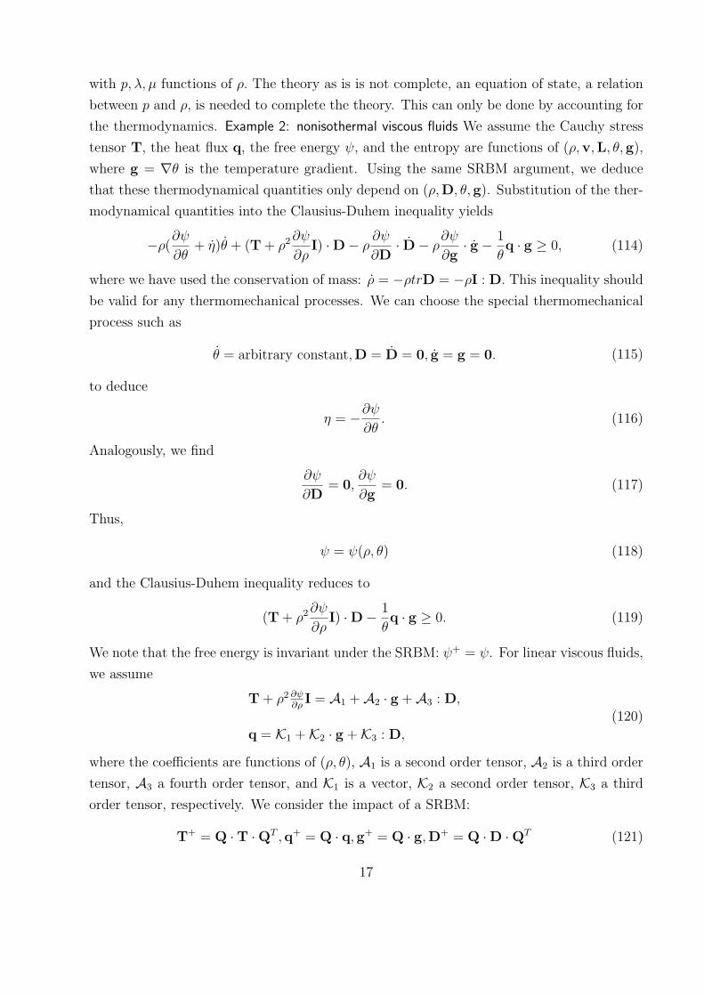
with p, λ, µ functions of ρ. The theory as is is not complete, an equation of state, a relation

between p and ρ, is needed to complete the theory. This can only be done by accounting for

the thermodynamics. Example 2: nonisothermal viscous fluids We assume the Cauchy stress

tensor T, the heat flux q, the free energy ψ, and the entropy are functions of (ρ,v,L, θ,g),

where g = ∇θ is the temperature gradient. Using the same SRBM argument, we deduce

that these thermodynamical quantities only depend on (ρ,D, θ,g). Substitution of the ther-

modynamical quantities into the Clausius-Duhem inequality yields

−ρ(∂ψ∂θ

+ η)θ + (T + ρ2∂ψ

∂ρI) ·D− ρ

∂ψ

∂D· D− ρ

∂ψ

∂g· g − 1

θq · g ≥ 0, (114)

where we have used the conservation of mass: ρ = −ρtrD = −ρI : D. This inequality should

be valid for any thermomechanical processes. We can choose the special thermomechanical

process such as

θ = arbitrary constant,D = D = 0, g = g = 0. (115)

to deduce

η = −∂ψ∂θ. (116)

Analogously, we find

∂ψ

∂D= 0,

∂ψ

∂g= 0. (117)

Thus,

ψ = ψ(ρ, θ) (118)

and the Clausius-Duhem inequality reduces to

(T + ρ2∂ψ

∂ρI) ·D− 1

θq · g ≥ 0. (119)

We note that the free energy is invariant under the SRBM: ψ+ = ψ. For linear viscous fluids,

we assume

T + ρ2 ∂ψ∂ρ

I = A1 +A2 · g +A3 : D,

q = K1 +K2 · g +K3 : D,

(120)

where the coefficients are functions of (ρ, θ), A1 is a second order tensor, A2 is a third order

tensor, A3 a fourth order tensor, and K1 is a vector, K2 a second order tensor, K3 a third

order tensor, respectively. We consider the impact of a SRBM:

T+ = Q ·T ·QT ,q+ = Q · q,g+ = Q · g,D+ = Q ·D ·QT (121)

17

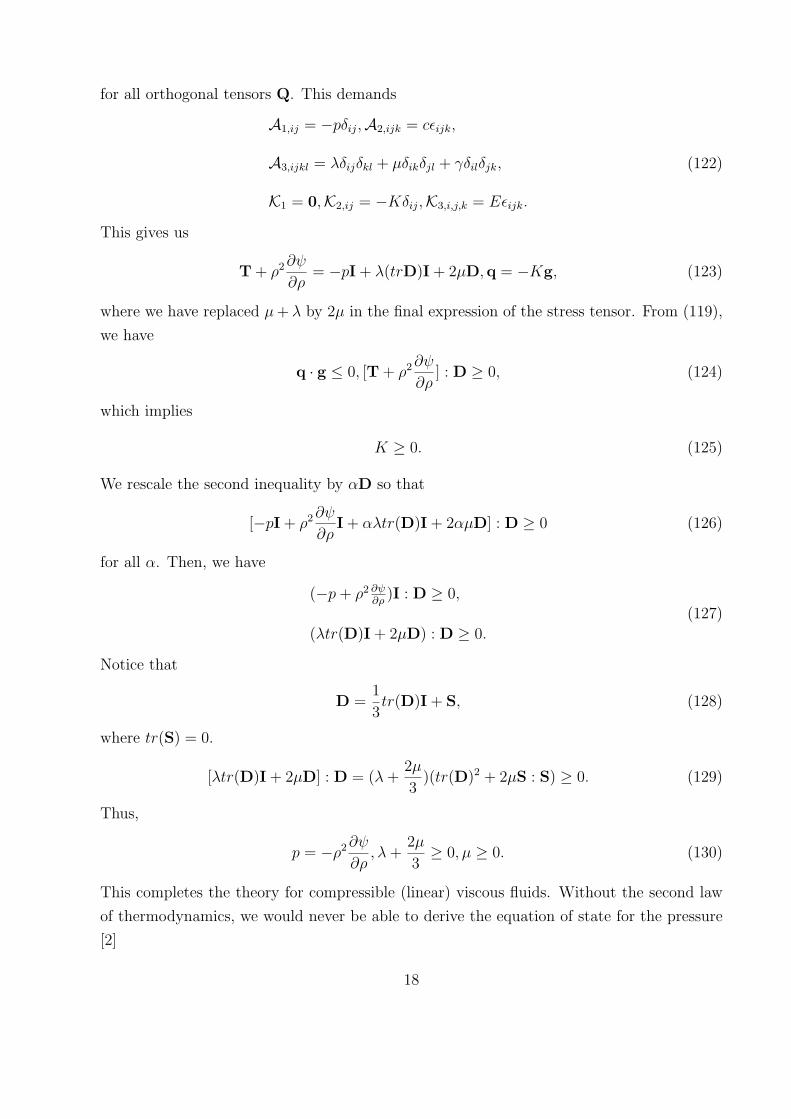
for all orthogonal tensors Q. This demands

A1,ij = −pδij,A2,ijk = cεijk,

A3,ijkl = λδijδkl + µδikδjl + γδilδjk,

K1 = 0,K2,ij = −Kδij,K3,i,j,k = Eεijk.

(122)

This gives us

T + ρ2∂ψ

∂ρ= −pI + λ(trD)I + 2µD,q = −Kg, (123)

where we have replaced µ+ λ by 2µ in the final expression of the stress tensor. From (119),

we have

q · g ≤ 0, [T + ρ2∂ψ

∂ρ] : D ≥ 0, (124)

which implies

K ≥ 0. (125)

We rescale the second inequality by αD so that

[−pI + ρ2∂ψ

∂ρI + αλtr(D)I + 2αµD] : D ≥ 0 (126)

for all α. Then, we have

(−p+ ρ2 ∂ψ∂ρ

)I : D ≥ 0,

(λtr(D)I + 2µD) : D ≥ 0.

(127)

Notice that

D =1

3tr(D)I + S, (128)

where tr(S) = 0.

[λtr(D)I + 2µD] : D = (λ+2µ

3)(tr(D)2 + 2µS : S) ≥ 0. (129)

Thus,

p = −ρ2∂ψ

∂ρ, λ+

2µ

3≥ 0, µ ≥ 0. (130)

This completes the theory for compressible (linear) viscous fluids. Without the second law

of thermodynamics, we would never be able to derive the equation of state for the pressure

[2]

18

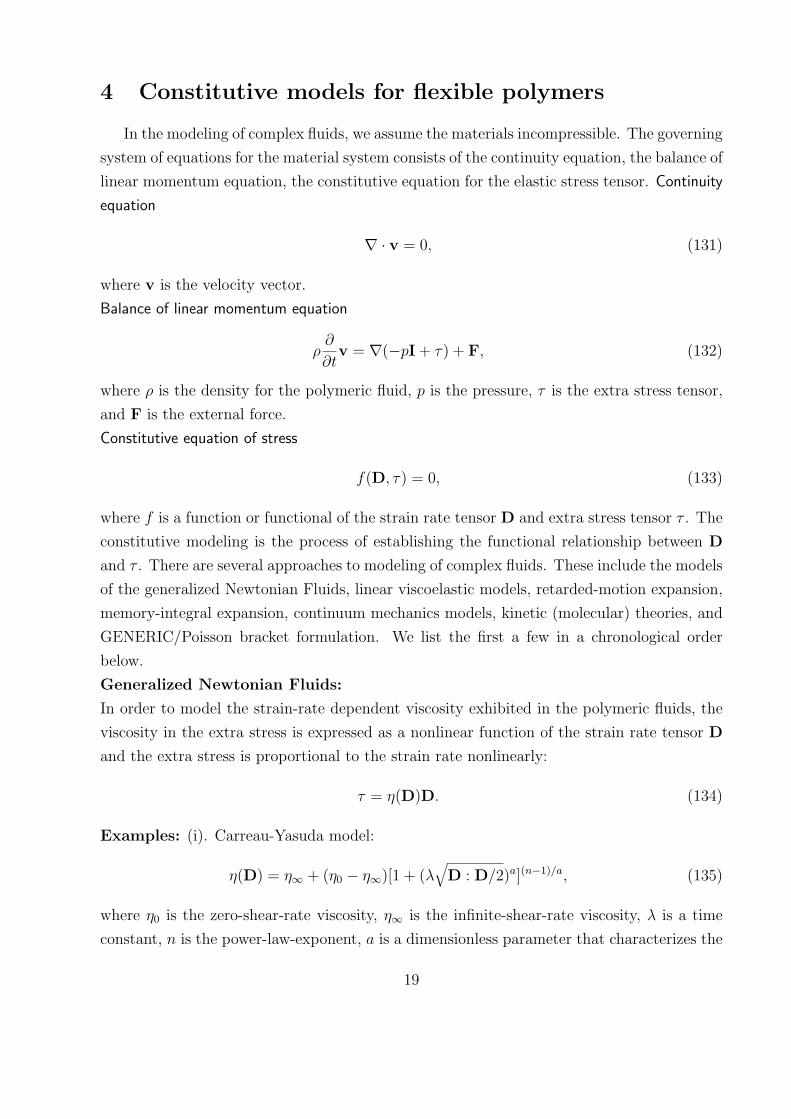
4 Constitutive models for flexible polymers

In the modeling of complex fluids, we assume the materials incompressible. The governing

system of equations for the material system consists of the continuity equation, the balance of

linear momentum equation, the constitutive equation for the elastic stress tensor. Continuity

equation

∇ · v = 0, (131)

where v is the velocity vector.

Balance of linear momentum equation

ρ∂

∂tv = ∇(−pI + τ) + F, (132)

where ρ is the density for the polymeric fluid, p is the pressure, τ is the extra stress tensor,

and F is the external force.

Constitutive equation of stress

f(D, τ) = 0, (133)

where f is a function or functional of the strain rate tensor D and extra stress tensor τ . The

constitutive modeling is the process of establishing the functional relationship between D

and τ . There are several approaches to modeling of complex fluids. These include the models

of the generalized Newtonian Fluids, linear viscoelastic models, retarded-motion expansion,

memory-integral expansion, continuum mechanics models, kinetic (molecular) theories, and

GENERIC/Poisson bracket formulation. We list the first a few in a chronological order

below.

Generalized Newtonian Fluids:

In order to model the strain-rate dependent viscosity exhibited in the polymeric fluids, the

viscosity in the extra stress is expressed as a nonlinear function of the strain rate tensor D

and the extra stress is proportional to the strain rate nonlinearly:

τ = η(D)D. (134)

Examples: (i). Carreau-Yasuda model:

η(D) = η∞ + (η0 − η∞)[1 + (λ√

D : D/2)a](n−1)/a, (135)

where η0 is the zero-shear-rate viscosity, η∞ is the infinite-shear-rate viscosity, λ is a time

constant, n is the power-law-exponent, a is a dimensionless parameter that characterizes the

19

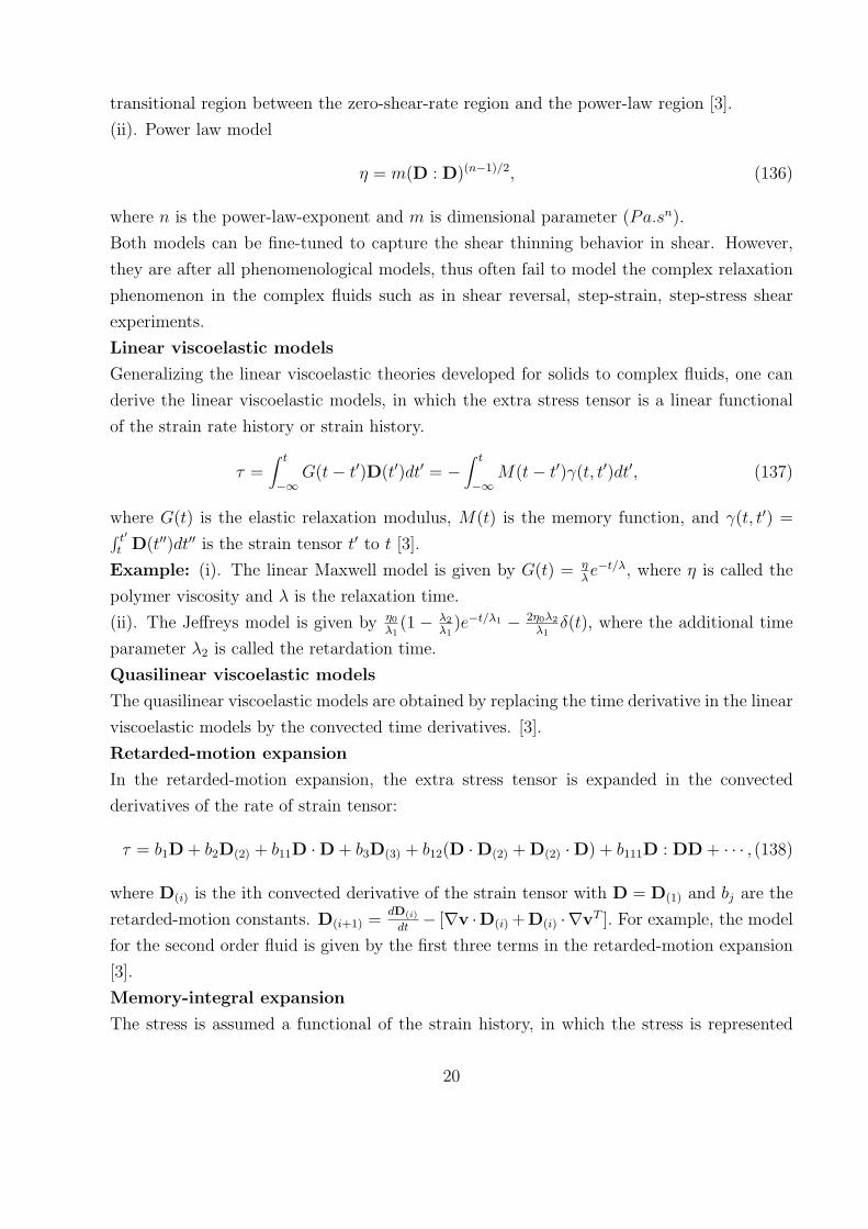
transitional region between the zero-shear-rate region and the power-law region [3].

(ii). Power law model

η = m(D : D)(n−1)/2, (136)

where n is the power-law-exponent and m is dimensional parameter (Pa.sn).

Both models can be fine-tuned to capture the shear thinning behavior in shear. However,

they are after all phenomenological models, thus often fail to model the complex relaxation

phenomenon in the complex fluids such as in shear reversal, step-strain, step-stress shear

experiments.

Linear viscoelastic models

Generalizing the linear viscoelastic theories developed for solids to complex fluids, one can

derive the linear viscoelastic models, in which the extra stress tensor is a linear functional

of the strain rate history or strain history.

τ =∫ t

−∞G(t− t′)D(t′)dt′ = −

∫ t

−∞M(t− t′)γ(t, t′)dt′, (137)

where G(t) is the elastic relaxation modulus, M(t) is the memory function, and γ(t, t′) =∫ t′t D(t′′)dt′′ is the strain tensor t′ to t [3].

Example: (i). The linear Maxwell model is given by G(t) = ηλe−t/λ, where η is called the

polymer viscosity and λ is the relaxation time.

(ii). The Jeffreys model is given by η0λ1

(1 − λ2

λ1)e−t/λ1 − 2η0λ2

λ1δ(t), where the additional time

parameter λ2 is called the retardation time.

Quasilinear viscoelastic models

The quasilinear viscoelastic models are obtained by replacing the time derivative in the linear

viscoelastic models by the convected time derivatives. [3].

Retarded-motion expansion

In the retarded-motion expansion, the extra stress tensor is expanded in the convected

derivatives of the rate of strain tensor:

τ = b1D + b2D(2) + b11D ·D + b3D(3) + b12(D ·D(2) + D(2) ·D) + b111D : DD + · · · , (138)

where D(i) is the ith convected derivative of the strain tensor with D = D(1) and bj are the

retarded-motion constants. D(i+1) =dD(i)

dt− [∇v ·D(i) +D(i) ·∇vT ]. For example, the model

for the second order fluid is given by the first three terms in the retarded-motion expansion

[3].

Memory-integral expansion

The stress is assumed a functional of the strain history, in which the stress is represented

20

as the Frechet series of the convected derivatives of the strain tensor. The retarded-motion

expansion can be derived from this more general method as a matter of fact.

τ = −∫ t−∞M(t− t′)γ(t′)dt′ −

∫ t−∞

∫ t−∞MII(t− t′, t− t′′)(γ′ · γ′′ + γ′′ · γ′)dt′′dt′+

∫ t−∞

∫ t−∞

∫ t−∞MIII(t− t′, t− t′′, t− t′′′)γ′γ′′ : γ′′′dt′′′dt′′dt′ + · · · ,

(139)

where γ′ = γ(t, t′) is the strain tensor and M’s are the memory functions [3].

Macroscopic models:

A large class of constitutive equations for the stress tensor can be written into the form

τ = 2ηD + τp,

τp + λτp + f(D, τp) = 2ηD,(140)

where

τp =dτpdt

− Ω · τp + τp · Ω− a[D · τp + τp ·D] (141)

is the Gordon-Schowalter derivative; a=-1: lower convected, a=1: upper convected, a=0:

corotational, is the vorticity tensor; the choice of f specifies the model. Examples: (i).

f=0 yields the Johnson Segalman model. (ii). f = cτ · τ gives the Giesekus model, where

c is a constant. (iii). f = cD : τ(τ + GI), where c and G are constants, gives the Larson

model. (iv). f = 0, λ = λ(√

D : D) and η = η(√

D : D) yield the white metzner model.

(v). Phan-Thien/Tanner model corresponds to f = Y (tr(τ))τ, where Y is a scalar function.

The Poisson bracket formulation and the Generic formulation can be found in the book [1]

5 Kinetic theory and the Rouse model for flexible poly-

mers

In this section, we give a crash course on the development of kinetic theories for polymeric

liquids. We derive the kinetic theory using a phenomenological approach, which can be called

a poor man’s kinetic theory. We begin with the conservation of polymer number density. This

is the most fundamental conservation law in the development of kinetic theories. Let ψ be

the number density of some polymer and F the flux of the polymer flow in the generalized

coordinate or phase space x. The conservation law for the number of polymers in any

”material volume” in the phase space yields

∂ψ

∂t+∂F

∂x= 0. (142)

Using the instantaneous velocity v at x, we can rewrite the flux as

F = vψ. (143)

21

Assume the motion of polymers are due to a force generated by an external field U and the

Brownian force. The inertialess force balance equation reads

L−1 · v +∂

∂xµ = 0, µ = kT lnρ+ U, (144)

where µ is the chemical potential and L−1 the friction coefficient matrix, which is assumed

invertible. Then,

v = −L · ∂µ∂x. (145)

(142) becomes

∂ψ

∂t− ∂

∂x· (L · ∂µ

∂xψ) = 0. (146)

This equation is called the Smoluchowski equation or the kinetic equation. For a system in

which the molecule is described by x = xiN1 , where xi ∈ R3, the Smoluchowski equation

is usually written as

∂ψ

∂t+

N∑n=1

∂

∂xn

· (vnψ) = 0,vn = −∑m

Lnm∂µ

∂xm

, (147)

where L = (Lnm) is the mobility matrix and Lnm = Lmn, (Lmn) > 0. When the particle

system x is immersed in a viscous solvent, each particle is going to be subject to a drag

exerted by the solvent and additional forces on each particle caused by the perturbation of

the flow field due to the motion of the particles. This is called the hydrodynamic effect.

When hydrodynamic effect is included, the total velocity consists of two parts:

vn = ven + vvn,ven = −

∑m

Lnm ·∂µ

∂xm, (148)

where the mobility matrix depends on the location of the particles and the second part vvn

is due to the existence of the macroscopic flow field and often it is well approximated by

vvn = ∇v · xn, (149)

where v is the averaged velocity field. We assume ∇v is a slowly varying function in space

in the length scale of the system x. Thus, in the process of finding the velocity due to

external forces, it is assumed a space-independent function. In the following, we assume the

particle is approximated by a sphere. Due to the presence and motion of the spheres, the

flow field around each particle is perturbed, which in turn affect the motion of the other

spheres. This phenomenon is called the hydrodynamic interaction. For very dilute solution

where the distance between spheres are sufficiently far so that the hydrodynamic interaction

22

can be neglected, the velocity of the sphere is determined by the external force acting on it

alone and the mobility matrix is given by

Lmn =δmnζ

I, (150)

where ζ = 6πηsa for spheres of radius a. In the general case, we have to solve the fluid

velocity v(x) with the given external force Fn exerted on the sphere at xn, which can be

expressed as

g(x) =∑n

Fnδ(x− xn). (151)

We simplify the problem by treating the sphere as a point mass. We assume the solvent is

incompressible ∇ · v = 0 and governed by the Stokes equation

∇ · τ + g = 0, (152)

where the stress tensor is given by

τ = −p+ 2ηsD. (153)

A solution of the equation is

v = K · x +∑m

H(x− xm) · Fm, (154)

where K = ∇v is treated as a spatially homogeneous tensor and

H(x) =1

8ηsπx(I +

xx

x2) (155)

is called the Oseen tensor, where x = ‖x‖. This tensor is singular at x = 0, which is due to

the assumption that the particle is a point. For finite size sphere, this singularity would be

removed. However, the exact solution of the stokes equation is not feasible. A compromise

is to approximate the Oseen tensor for point mass by

H(x) =

Iζ, x = 0,

H(x), x 6= 0.(156)

The mobility matrix is then calculated by

Lmn = H(xn − xm). (157)

The Smoluchowski equation then becomes

∂ψ

∂t=

N∑n=1

∂

∂xn

· [∑m

Lnm∂µ

∂xm

−∇v · xn]. (158)

23

The elastic stress in the polymer system can be derived from a virtual work principle. Let

A =∫V

∫µψdxdv (159)

be the free energy over the material volume V . (We remark that this free energy formulation

is based on that the potential U is independent of ψ; if U depends on ψ as well, A has to be

modified such that δAδψ

= µ.) We consider an infinitesimal deformation given by

δψ =dψ

dtδt = −

∑n

∂

∂xn· [∇v · xn]δt. (160)

Take the variation of the free energy and assume vol(V ) small, we have

δA = vol(V )τ e : δt∇v = −δt∇vαβ∑n

〈Fnαxnβ〉, (161)

where

Fn = − ∂µ

∂xn(162)

is the force exerted on the part of the polymer at xn. The elastic part of stress is then given

by

τ e = − 1

vol(V )

∑n

〈Fnxn〉, (163)

where

〈(•)〉 =∫V

∫(•)dxdv. (164)

5.1 Langevin equation

An alternative description of the molecular motion is the Langevin equation. For each

particle xn, there is a stochastic differential equation

xn =∑m

Lnm(− ∂U

∂xn+ fm(t)) +

1

2kT

∂

∂xmLnm, (165)

where fm(t) is a random force subject to the Gaussian distribution and

〈fm〉 = 0, 〈fnfm〉 = 2(L−1)nmkTδ(t− t′). (166)

This Langevin equation implies the Smoluchowski equation. Lemma: The Langevin equation

dx

dt= −1

ξ

∂

∂xU(x) +

√kT

ξg(t) +

1

2

d

dx(kT

ξ) (167)

implies the distribution density function of x satisfies

∂

∂tψ =

∂

∂x

1

ξ(kT

∂

∂xψ +

∂U

∂xψ) =

∂

∂x

1

ξ(∂

∂xµψ), (168)

where

〈g(t)〉 = 0, 〈g(t)g(t′)〉 = 2δ(t− t′). (169)

24

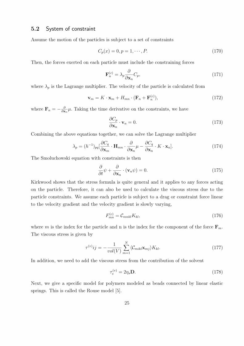
5.2 System of constraint

Assume the motion of the particles is subject to a set of constraints

Cp(x) = 0, p = 1, · · · , P. (170)

Then, the forces exerted on each particle must include the constraining forces

F(c)n = λp

∂

∂xnCp, (171)

where λp is the Lagrange multiplier. The velocity of the particle is calculated from

vm = K · xm +Hmn · (Fn + F(c)n ), (172)

where Fn = − ∂∂xn

µ. Taking the time derivative on the constraints, we have

∂Cp∂xn

· vn = 0. (173)

Combining the above equations together, we can solve the Lagrange multiplier

λp = (h−1)pq[∂Cq∂xm

·Hmn ·∂

∂xnµ− ∂Cq

∂xn·K · xn]. (174)

The Smoluchowski equation with constraints is then

∂

∂tψ +

∂

∂xn· (vnψ) = 0. (175)

Kirkwood shows that the stress formula is quite general and it applies to any forces acting

on the particle. Therefore, it can also be used to calculate the viscous stress due to the

particle constraints. We assume each particle is subject to a drag or constraint force linear

to the velocity gradient and the velocity gradient is slowly varying,

F (c)mn = CmnklKkl, (176)

where m is the index for the particle and n is the index for the component of the force Fm.

The viscous stress is given by

τ (v)ij = − 1

vol(V )

N∑m=1

〈Cmiklxmj〉Kkl. (177)

In addition, we need to add the viscous stress from the contribution of the solvent

τ (v)s = 2ηsD. (178)

Next, we give a specific model for polymers modeled as beads connected by linear elastic

springs. This is called the Rouse model [5].

25

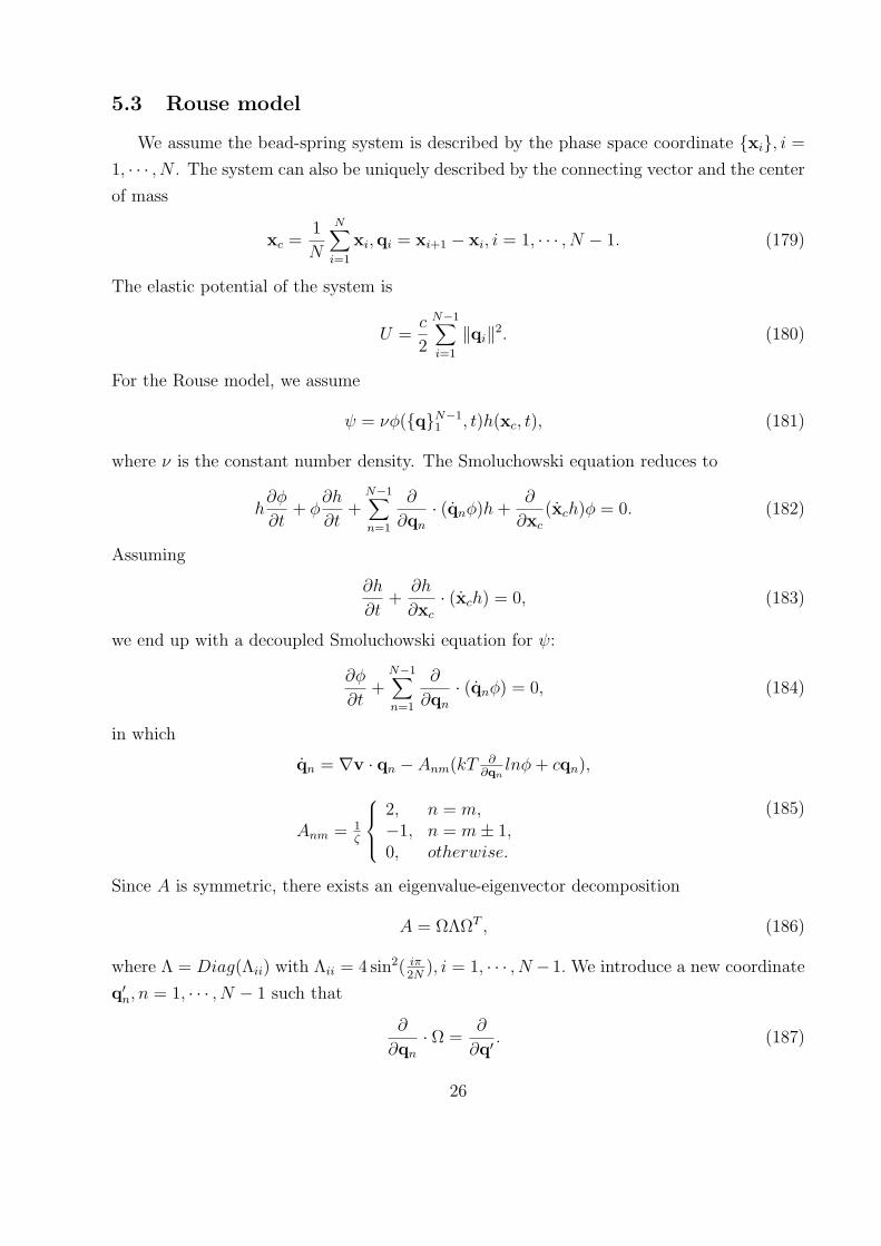
5.3 Rouse model

We assume the bead-spring system is described by the phase space coordinate xi, i =

1, · · · , N . The system can also be uniquely described by the connecting vector and the center

of mass

xc =1

N

N∑i=1

xi,qi = xi+1 − xi, i = 1, · · · , N − 1. (179)

The elastic potential of the system is

U =c

2

N−1∑i=1

‖qi‖2. (180)

For the Rouse model, we assume

ψ = νφ(qN−11 , t)h(xc, t), (181)

where ν is the constant number density. The Smoluchowski equation reduces to

h∂φ

∂t+ φ

∂h

∂t+

N−1∑n=1

∂

∂qn· (qnφ)h+

∂

∂xc(xch)φ = 0. (182)

Assuming

∂h

∂t+∂h

∂xc· (xch) = 0, (183)

we end up with a decoupled Smoluchowski equation for ψ:

∂φ

∂t+

N−1∑n=1

∂

∂qn· (qnφ) = 0, (184)

in which

qn = ∇v · qn − Anm(kT ∂∂qn

lnφ+ cqn),

Anm = 1ζ

2, n = m,−1, n = m± 1,0, otherwise.

(185)

Since A is symmetric, there exists an eigenvalue-eigenvector decomposition

A = ΩΛΩT , (186)

where Λ = Diag(Λii) with Λii = 4 sin2( iπ2N

), i = 1, · · · , N −1. We introduce a new coordinate

q′n, n = 1, · · · , N − 1 such that

∂

∂qn· Ω =

∂

∂q′. (187)

26

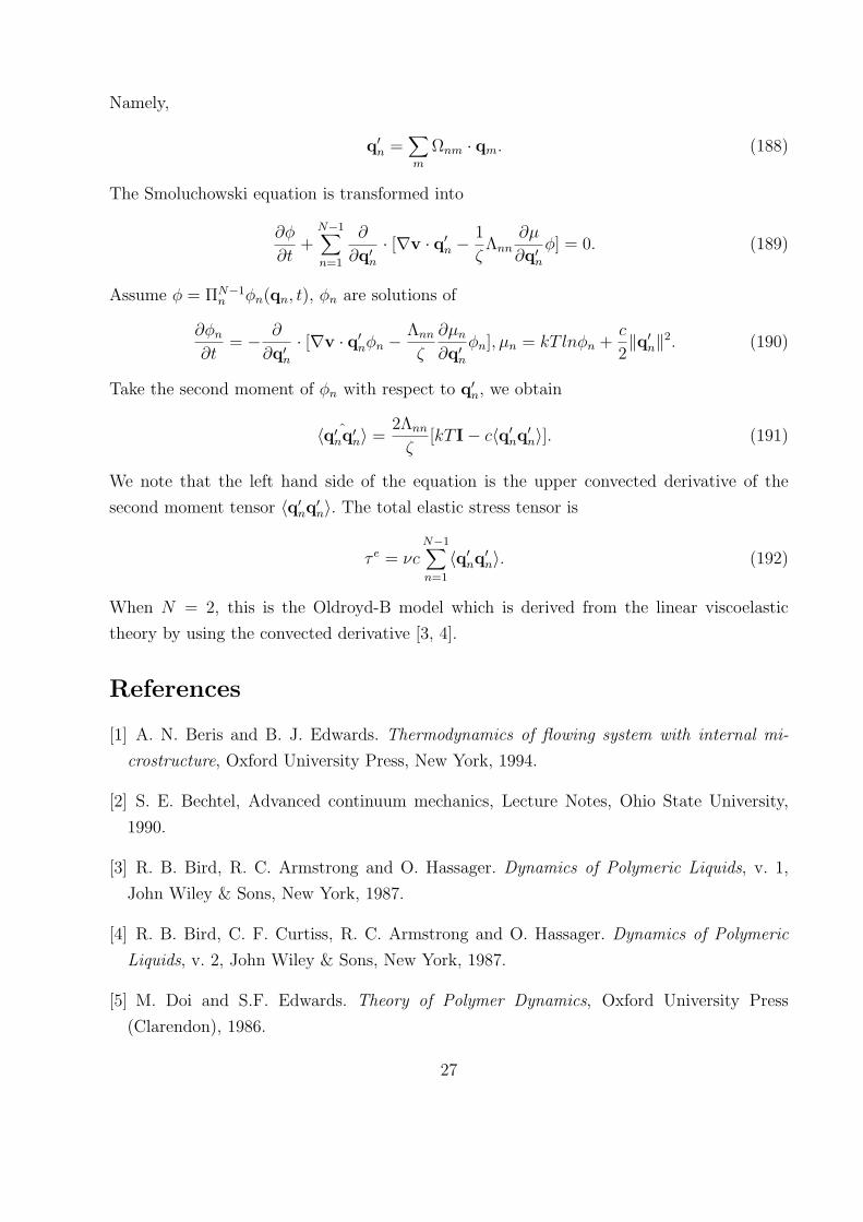
Namely,

q′n =∑m

Ωnm · qm. (188)

The Smoluchowski equation is transformed into

∂φ

∂t+

N−1∑n=1

∂

∂q′n· [∇v · q′n −

1

ζΛnn

∂µ

∂q′nφ] = 0. (189)

Assume φ = ΠN−1n φn(qn, t), φn are solutions of

∂φn∂t

= − ∂

∂q′n· [∇v · q′nφn −

Λnn

ζ

∂µn∂q′n

φn], µn = kT lnφn +c

2‖q′n‖2. (190)

Take the second moment of φn with respect to q′n, we obtain

ˆ〈q′nq′n〉 =2Λnn

ζ[kT I− c〈q′nq′n〉]. (191)

We note that the left hand side of the equation is the upper convected derivative of the

second moment tensor 〈q′nq′n〉. The total elastic stress tensor is

τ e = νcN−1∑n=1

〈q′nq′n〉. (192)

When N = 2, this is the Oldroyd-B model which is derived from the linear viscoelastic

theory by using the convected derivative [3, 4].

References

[1] A. N. Beris and B. J. Edwards. Thermodynamics of flowing system with internal mi-

crostructure, Oxford University Press, New York, 1994.

[2] S. E. Bechtel, Advanced continuum mechanics, Lecture Notes, Ohio State University,

1990.

[3] R. B. Bird, R. C. Armstrong and O. Hassager. Dynamics of Polymeric Liquids, v. 1,

John Wiley & Sons, New York, 1987.

[4] R. B. Bird, C. F. Curtiss, R. C. Armstrong and O. Hassager. Dynamics of Polymeric

Liquids, v. 2, John Wiley & Sons, New York, 1987.

[5] M. Doi and S.F. Edwards. Theory of Polymer Dynamics, Oxford University Press

(Clarendon), 1986.

27

[6] A. C. Eringen, Mechanics of Continua, Robert E. Krieger Publishing Company, Malabar,

Florida, 1980.

[7] A. C. Eringen, Microcontinuum Field Theories I: Foundations and Solids, II: Fluent

Media, Springer-Verlag, New York, 1999.

[8] R. G. Larson. The structure and Rheology of Complex Fluids, Oxford University Press,

1999.

[9] R. G. Larson. Constitutive Equations for Polymer Melts and Solutions, Butterworths,

Boston, 1988.

28