SOLID MECHANICSpiet/edu/som/pdf/somsht1516_3.pdf · Elasticity models σ ε constitutive equation...

SOLID MECHANICS

Piet Schreurs

Department of Mechanical EngineeringEindhoven University of Technology

http://www.mate.tue.nl/∼piet

2015/2016

March 11, 2016

INDEX

Nonlinear deformation

One-dimensional material behavior

Elastic

Elastoplastic

Piet Schreurs (TU/e) 2 / 54

NONLINEAR TRUSS

back to index

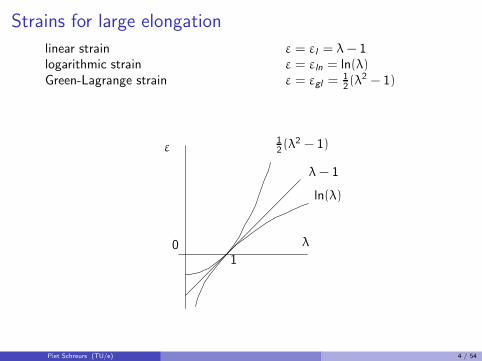
Strains for large elongation

linear strain ε = εl = λ − 1logarithmic strain ε = εln = ln(λ)

Green-Lagrange strain ε = εgl = 12(λ2 − 1)

12 (λ2 − 1)

λ − 1

ln(λ)

ε

λ

10


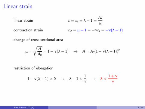
Linear strain

linear strain ε = εl = λ − 1 =∆l

l0

contraction strain εd = µ − 1 = −νεl = −ν(λ − 1)

change of cross-sectional area

µ =

√

A

A0= 1 − ν(λ − 1) → A = A0{1 − ν(λ − 1)}2

restriction of elongation

1 − ν(λ − 1) > 0 → λ − 1 <1

ν→ λ <

1 + ν

ν


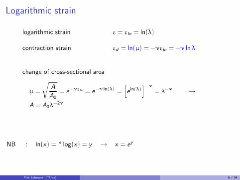
Logarithmic strain

logarithmic strain ε = εln = ln(λ)

contraction strain εd = ln(µ) = −νεln = −ν lnλ


µ =

√

A

A0= e−νεln = e−ν ln(λ) =

[

e ln(λ)]−ν

= λ−ν →

A = A0λ−2ν

NB : ln(x) = e log(x) = y → x = ey


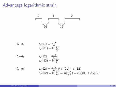
Advantage logarithmic strain

1 2

01 12

0

l0→l1 εl (01) = l1−l0l0

εln(01) = ln( l1l0)

l1→l2 εl (12) = l2−l1l1

εln(12) = ln( l2l1)

l0→l2 εl (02) = l2−l0l0

6= εl(01) + εl(12)

εln(02) = ln( l2l0) = ln( l2

l1

l1l0) = εln(01) + εln(12)


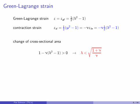
Green-Lagrange strain

Green-Lagrange strain ε = εgl = 12 (λ2 − 1)

contraction strain εd = 12 (µ2 − 1) = −νεln = −ν 1

2 (λ2 − 1)


1 − ν(λ2 − 1) > 0 → λ <

√

1 + ν

ν


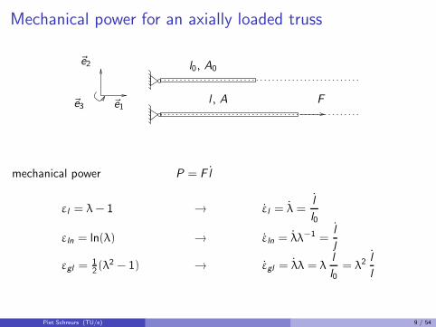
Mechanical power for an axially loaded truss

l0, A0

l , A F~e1

~e2

~e3

mechanical power P = F l

εl = λ − 1 → εl = λ =l

l0

εln = ln(λ) → εln = λλ−1 =l

l

εgl = 12 (λ2 − 1) → εgl = λλ = λ

l

l0= λ2 l

l


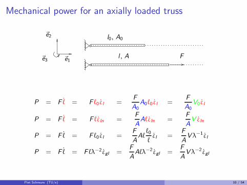
Mechanical power for an axially loaded truss

l0, A0

l , A F~e1

~e2

~e3

P = F ℓ = F ℓ0εl =F

A0A0ℓ0εl =

F

A0V0εl

P = F ℓ = F ℓεln =F

AAℓεln =

F

AV εln

P = F ℓ = F ℓ0εl =F

AAℓ

ℓ0

ℓεl =

F

AVλ−1εl

P = F ℓ = F ℓλ−2εgl =F

AAℓλ−2εgl =

F

AVλ−2εgl


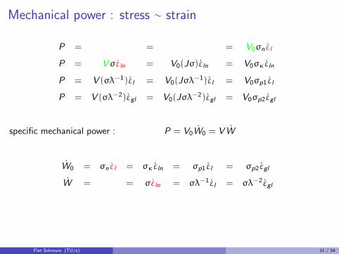
Mechanical power : stress ∼ strain

P = = = V0σn εl

P = Vσεln = V0(Jσ)εln = V0σκεln

P = V (σλ−1)εl = V0(Jσλ−1)εl = V0σp1εl

P = V (σλ−2)εgl = V0(Jσλ−2)εgl = V0σp2εgl

specific mechanical power : P = V0W0 = VW

W0 = σn εl = σκεln = σp1εl = σp2εgl

W = = σεln = σλ−1εl = σλ−2εgl


SOLUTION PROCEDURE

back to index

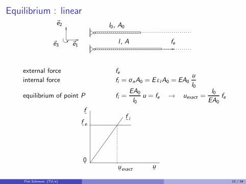
Equilibrium : linear

l0, A0

l , A fe~e1

~e2

~e3

external force fe

internal force fi = σnA0 = EεlA0 = EA0u

l0

equilibrium of point P fi =EA0

l0u = fe → uexact =

l0

EA0fe

f˜

if˜

e

f˜

u˜

u˜

exact

0˜


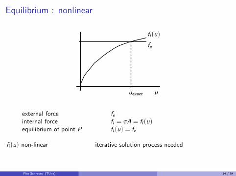
Equilibrium : nonlinear

u

fi (u)

fe

uexact

external force feinternal force fi = σA = fi (u)

equilibrium of point P fi (u) = fe

fi (u) non-linear iterative solution process needed


Iterative solution procedure

uu∗

f ∗i

fi (u)

r∗fe

uexact

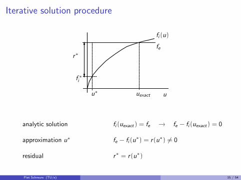
analytic solution fi (uexact ) = fe → fe − fi (uexact) = 0

approximation u∗ fe − fi (u∗) = r(u∗) 6= 0

residual r∗ = r(u∗)


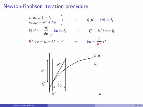
Newton-Raphson iteration procedure

fi (uexact) = feuexact = u∗ + δu

}

→ fi (u∗ + δu) = fe

fi (u∗) +

dfi

du

∣

∣

∣

∣

u∗

δu = fe → f ∗

i + K ∗δu = fe

K ∗ δu = fe − f ∗i = r∗ → δu =1

K ∗r∗

u

δu

u∗

K ∗

f ∗

i

fi (u)

fe

r∗


New approximate solution

uexact

δu

u∗

K ∗

f ∗

i

fi (u)

fe

r∗

uu∗∗

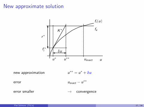
new approximation u∗∗ = u∗ + δu

error uexact − u∗∗

error smaller → convergence


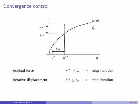
Convergence control

δu

u∗

fi (u)

r∗∗

u

fe

f ∗∗i

u∗∗

residual force |r∗∗| ≤ cr → stop iteration

iterative displacement |δu| ≤ cu → stop iteration


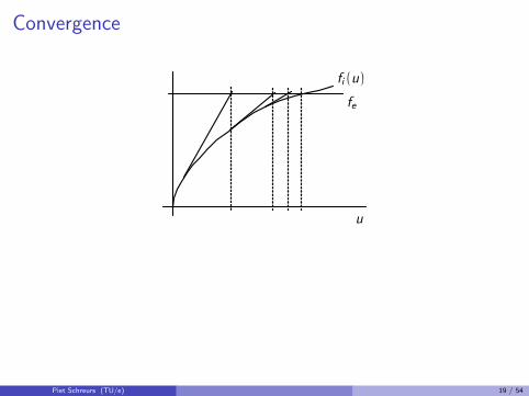
Convergence

u

fi (u)

fe


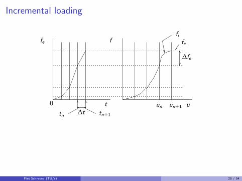
Incremental loading

fe

t0

fife

tn tn+1∆t

∆fe

f

un un+1 u


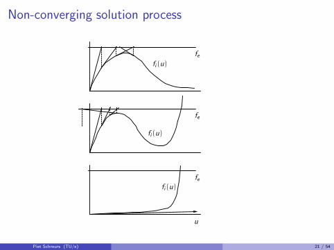
Non-converging solution process

fi (u)

fe

u

fe

fi (u)

fi (u)

fe


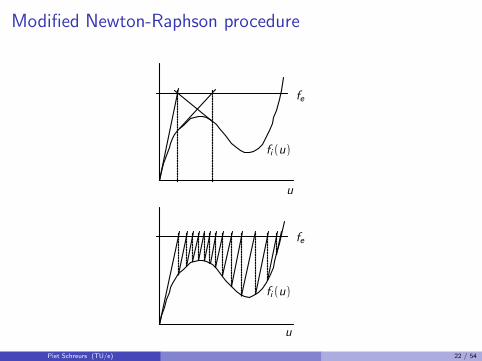
Modified Newton-Raphson procedure

u

u

fi (u)

fi (u)

fe

fe


ONE-DIMENSIONAL MATERIAL BEHAVIOR

back to index

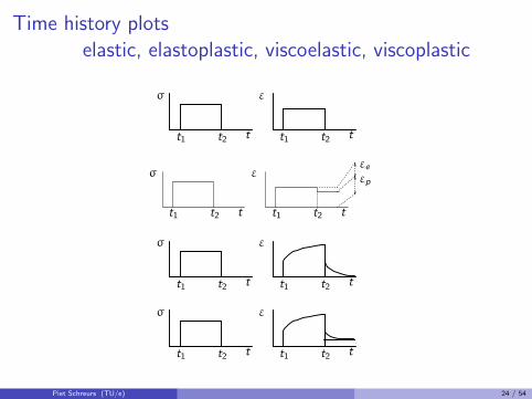
Time history plots

elastic, elastoplastic, viscoelastic, viscoplastic

t t

ε

t2

σ

t1 t2 t1

t t

εσ

t1 t2 t1 t2

εe

εp

t t2 t

εσ

t1 t2 t1

t2t t

εσ

t1 t2 t1


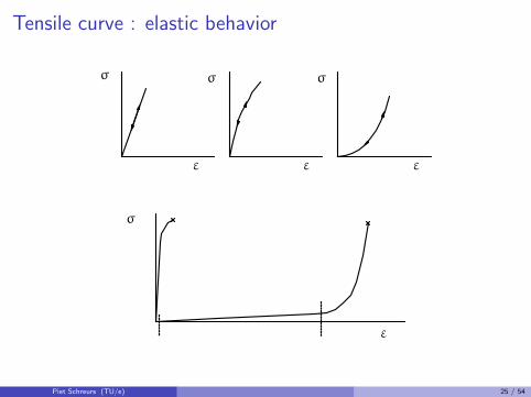
Tensile curve : elastic behavior

σ

ε

σ

ε

σ

ε

ε

σ


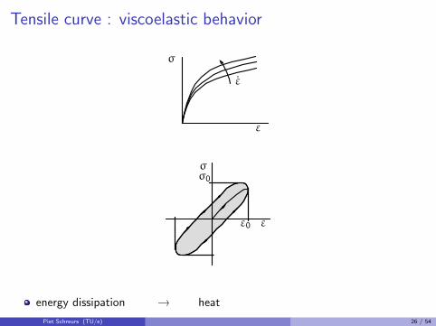
Tensile curve : viscoelastic behavior

ε

ε

σ

ε

σ

ε0

σ0

energy dissipation → heat


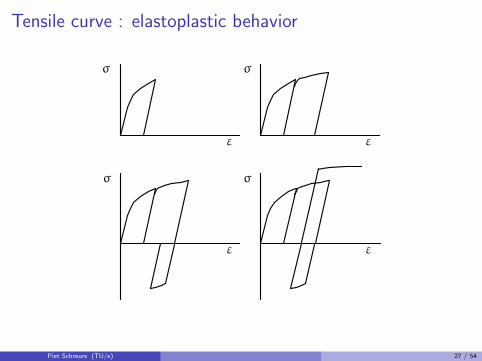
Tensile curve : elastoplastic behavior

σ

εε

σσ

σ

ε ε


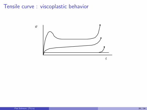
Tensile curve : viscoplastic behavior

ε

σ


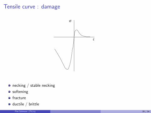
Tensile curve : damage

ε

σ

necking / stable necking

softening

fracture

ductile / brittle


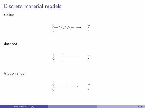
Discrete material models

spring

σε

dashpot

σε

friction slider

σε


ELASTIC

back to index

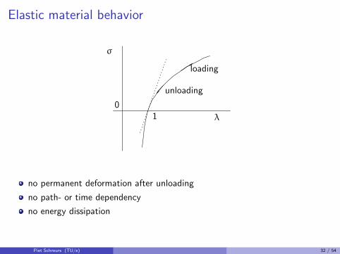
Elastic material behavior

unloading

loading

0

σ

λ1

no permanent deformation after unloading

no path- or time dependency

no energy dissipation


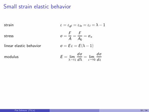
Small strain elastic behavior

strain ε = εgl = εln = εl = λ − 1

stress σ =F

A=

F

A0= σn

linear elastic behavior σ = Eε = E (λ − 1)

modulus E = limλ→1

dσ

dλ= lim

ε→0

dσ

dε


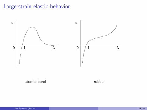
Large strain elastic behavior

σ

0 1 λ

atomic bond

σ

0 1 λ

rubber


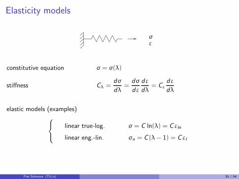
Elasticity models

σε

constitutive equation σ = σ(λ)

stiffness Cλ =dσ

dλ=

dσ

dε

dε

dλ= Cε

dε

dλ

elastic models (examples)

linear true-log. σ = C ln(λ) = Cεln

linear eng.-lin. σn = C (λ − 1) = Cεl


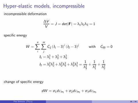
Hyper-elastic models, incompressible

incompressible deformation

∆V

V= J = det(F) = λ1λ2λ3 = 1

specific energy

W =

n∑

i

m∑

j

Cij (I1 − 3)i(I2 − 3)

jwith C00 = 0

I1 = λ21 + λ2

2 + λ23

I2 = λ21λ

22 + λ2

2λ23 + λ2

3λ21 =

1

λ23

+1

λ21

+1

λ22

change of specific energy

dW = σ1dεln1 + σ2dεln2 + σ3dεln3


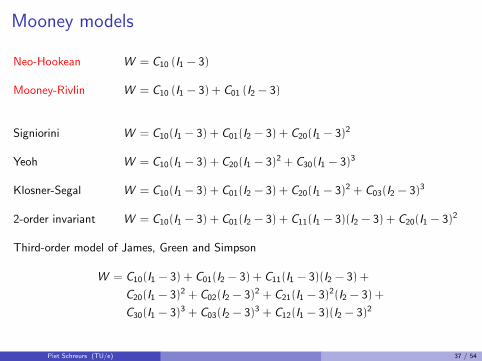
Mooney models

Neo-Hookean W = C10 (I1 − 3)

Mooney-Rivlin W = C10 (I1 − 3) + C01 (I2 − 3)

Signiorini W = C10(I1 − 3) + C01(I2 − 3) + C20(I1 − 3)2

Yeoh W = C10(I1 − 3) + C20(I1 − 3)2 + C30(I1 − 3)3

Klosner-Segal W = C10(I1 − 3) + C01(I2 − 3) + C20(I1 − 3)2 + C03(I2 − 3)3

2-order invariant W = C10(I1 − 3) + C01(I2 − 3) + C11(I1 − 3)(I2 − 3) + C20(I1 − 3)2

Third-order model of James, Green and Simpson

W = C10(I1 − 3) + C01(I2 − 3) + C11(I1 − 3)(I2 − 3) +

C20(I1 − 3)2 + C02(I2 − 3)2 + C21(I1 − 3)2(I2 − 3) +

C30(I1 − 3)3 + C03(I2 − 3)3 + C12(I1 − 3)(I2 − 3)2


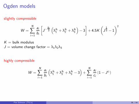
Ogden models

slightly compressible

W =

N∑

i=1

ai

bi

[

J−bi

3

(

λbi

1 + λbi

2 + λbi

3

)

− 3

]

+ 4.5K

(

J13 − 1

)2

K = bulk modulusJ = volume change factor = λ1λ2λ3

highly compressible

W =

N∑

i=1

ai

bi

(

λbi

1 + λbi

2 + λbi

3 − 3)

+

N∑

i=1

ai

ci

(1 − Jci )


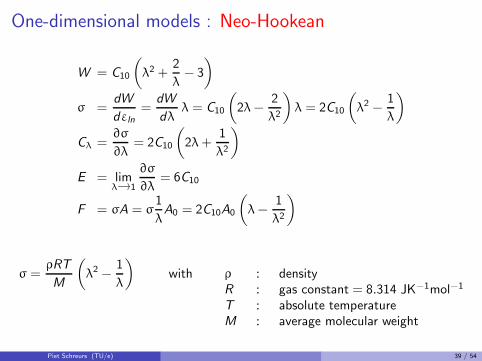
One-dimensional models : Neo-Hookean

W = C10

(

λ2 +2

λ− 3

)

σ =dW

dεln

=dW

dλλ = C10

(

2λ −2

λ2

)

λ = 2C10

(

λ2 −1

λ

)

Cλ =∂σ

∂λ= 2C10

(

2λ +1

λ2

)

E = limλ→1

∂σ

∂λ= 6C10

F = σA = σ1

λA0 = 2C10A0

(

λ −1

λ2

)

σ =ρRT

M

(

λ2 −1

λ

)

with ρ : densityR : gas constant = 8.314 JK−1mol−1

T : absolute temperatureM : average molecular weight


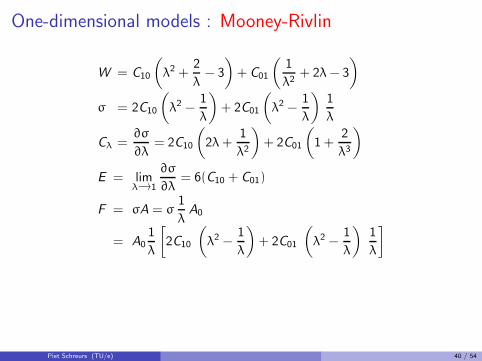
One-dimensional models : Mooney-Rivlin

W = C10

(

λ2 +2

λ− 3

)

+ C01

(

1

λ2+ 2λ − 3

)

σ = 2C10

(

λ2 −1

λ

)

+ 2C01

(

λ2 −1

λ

)

1

λ

Cλ =∂σ

∂λ= 2C10

(

2λ +1

λ2

)

+ 2C01

(

1 +2

λ3

)

E = limλ→1

∂σ

∂λ= 6(C10 + C01)

F = σA = σ1

λA0

= A01

λ

[

2C10

(

λ2 −1

λ

)

+ 2C01

(

λ2 −1

λ

)

1

λ

]


ELASTOPLASTIC

back to index

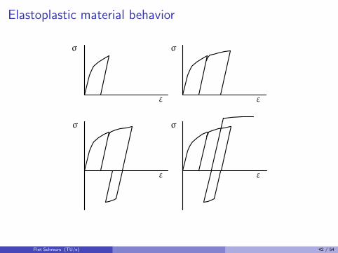
Elastoplastic material behavior

σ

εε

σσ

σ

ε ε


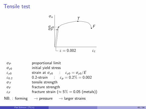
Tensile test

T

F

ε = 0.002 εℓ

σn

σPσy0

σP proportional limitσy0 initial yield stressεy0 strain at σy0 : εy0 = σy0/E

ε0.2 0.2-strain : εp = 0.2% = 0.002σT tensile strengthσF fracture strengthεF fracture strain (≈ 5% = 0.05 (metals))

NB. : forming → pressure → larger strains


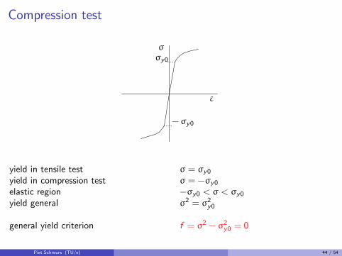
Compression test

σ

ε

σy0

− σy0

yield in tensile test σ = σy0

yield in compression test σ = −σy0

elastic region −σy0 < σ < σy0

yield general σ2 = σ2y0

general yield criterion f = σ2 − σ2y0 = 0


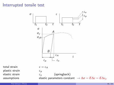
Interrupted tensile test

t t

εσ

t1 t2 t1 t2

εe

εp

ε

σ

σy0

εeεp

εA

A

B

σy

total strain ε = εA

plastic strain εp

elastic strain εe (springback)assumptions elastic parameters constant → ∆σ = E∆ε = E∆εe


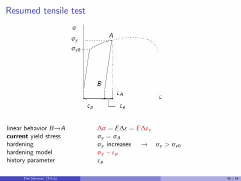
Resumed tensile test

ε

σ

σy0

εeεp

εA

A

B

σy

linear behavior B→A ∆σ = E∆ε = E∆εe

current yield stress σy = σA

hardening σy increases → σy > σy0

hardening model σy ∼ εp

history parameter εp


Hardening

A

B

A ′

Y0

Y ′

0

0ε

σ

q

A ′

Aσ

0

Y ′

0

Y0

B

C

ε

σy0

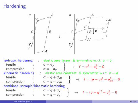
isotropic hardening : elastic area larger & symmetric w.r.t. σ = 0tensile : σ = σy

compression : σ = −σy

}

→ f = σ2 − σ2y = 0

kinematic hardening : elastic area constant & symmetric w.r.t. σ = qtensile : σ = q + σy0

compression : σ = q − σy0

}

→ f = (σ − q)2 − σ2y0 = 0

combined isotropic/kinematic hardeningtensile : σ = q + σy

compression : σ = q − σy

}

→ f = (σ − q)2 − σ2y = 0


Effective plastic strain

ε

t

A

B

CD

C

E

E

σ

ε

A

B

D

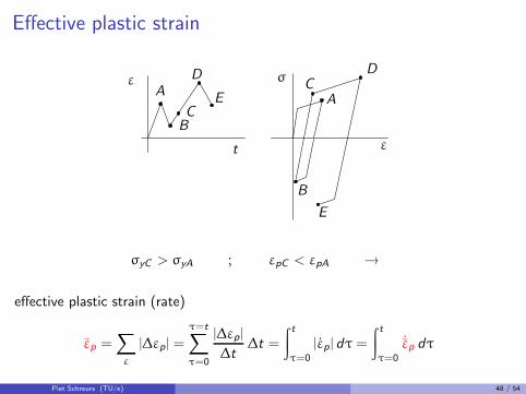
σyC > σyA ; εpC < εpA →

effective plastic strain (rate)

εp =∑

ε

|∆εp | =

τ=t∑

τ=0

|∆εp |

∆t∆t =

∫ t

τ=0

|εp | dτ =

∫ t

τ=0

˙εp dτ


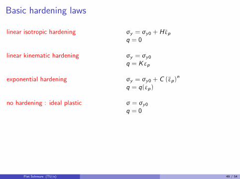
Basic hardening laws

linear isotropic hardening σy = σy0 + H εp

q = 0

linear kinematic hardening σy = σy0

q = Kεp

exponential hardening σy = σy0 + C (εp)n

q = q(εp)

no hardening : ideal plastic σ = σy0

q = 0


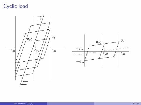
Cyclic load

εy0

σy0

εm

σ1

−εmεm

σm

εy0

σy0

−εm

−σm


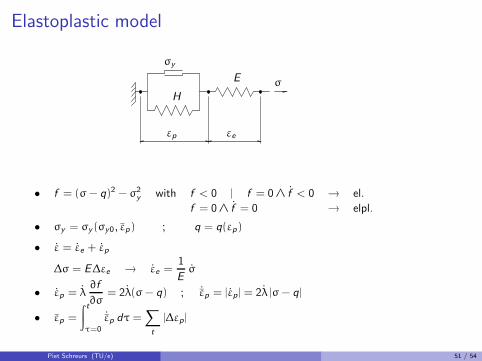
Elastoplastic model

H

σy

εeεp

σE

• f = (σ − q)2 − σ2y with f < 0 | f = 0 ∧ f < 0 → el.

f = 0 ∧ f = 0 → elpl.

• σy = σy (σy0, εp) ; q = q(εp)

• ε = εe + εp

∆σ = E∆εe → εe =1

Eσ

• εp = λ∂f

∂σ= 2λ(σ − q) ; ˙εp = |εp | = 2λ |σ − q|

• εp =

∫ t

τ=0

˙εp dτ =∑

t

|∆εp |


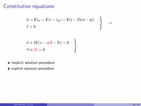
Constitutive equations

σ = E εe = E (ε − εp) = E {ε − 2λ(σ − q)}

f = 0

→

σ + 2E (σ − q)λ − E ε = 0

f (σ, λ) = 0

implicit solution procedure

explicit solution procedure


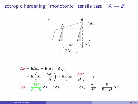
Isotropic hardening ”monotonic” tensile test A → B

∆εe

∆σσ

ε

∆ε

A

B

∆εp

∆σ = E∆εe = E (∆ε − ∆εp)

= E

(

∆ε −∆σy

H

)

= E

(

∆ε −∆σ

H

)

→

∆σ =EH

E + H∆ε = S∆ε ; ∆εp =

∆σ

H=

E

E + H∆ε


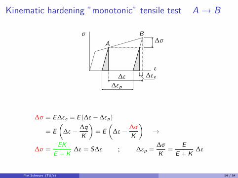
Kinematic hardening ”monotonic” tensile test A → B

∆εe

∆σσ

ε

∆ε

A

B

∆εp

∆σ = E∆εe = E (∆ε − ∆εp)

= E

(

∆ε −∆q

K

)

= E

(

∆ε −∆σ

K

)

→

∆σ =EK

E + K∆ε = S∆ε ; ∆εp =

∆σ

K=

E

E + K∆ε


SOLID MECHANICSpiet/edu/som/pdf/somsht1516_3.pdf · Elasticity models σ ε constitutive equation...

Documents

Transcript of SOLID MECHANICSpiet/edu/som/pdf/somsht1516_3.pdf · Elasticity models σ ε constitutive equation...