Advanced behavior models

Recent development of discrete choice models

Makoto Chikaraishi

Hiroshima University

October 13-15, 2017The 16th Summer Course for Behavior Modeling in Transportation Networks@The University of Tokyo

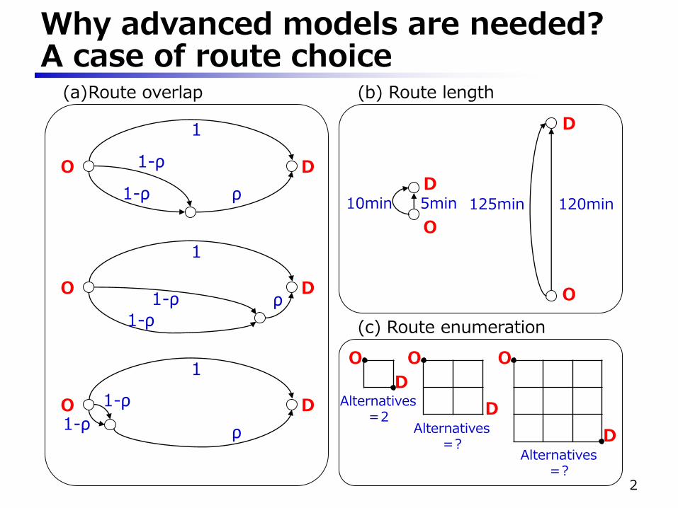
Why advanced models are needed?A case of route choice

O D

1

ρ1-ρ

1-ρ

O D

1

ρ1-ρ

1-ρ

O D

1

ρ

1-ρ

1-ρ

D

D

O

O

120min125min5min10min

(a)Route overlap (b) Route length

2

(c) Route enumeration

D

O

D

O

D

O

Alternatives＝2

Alternatives＝?

Alternatives＝?

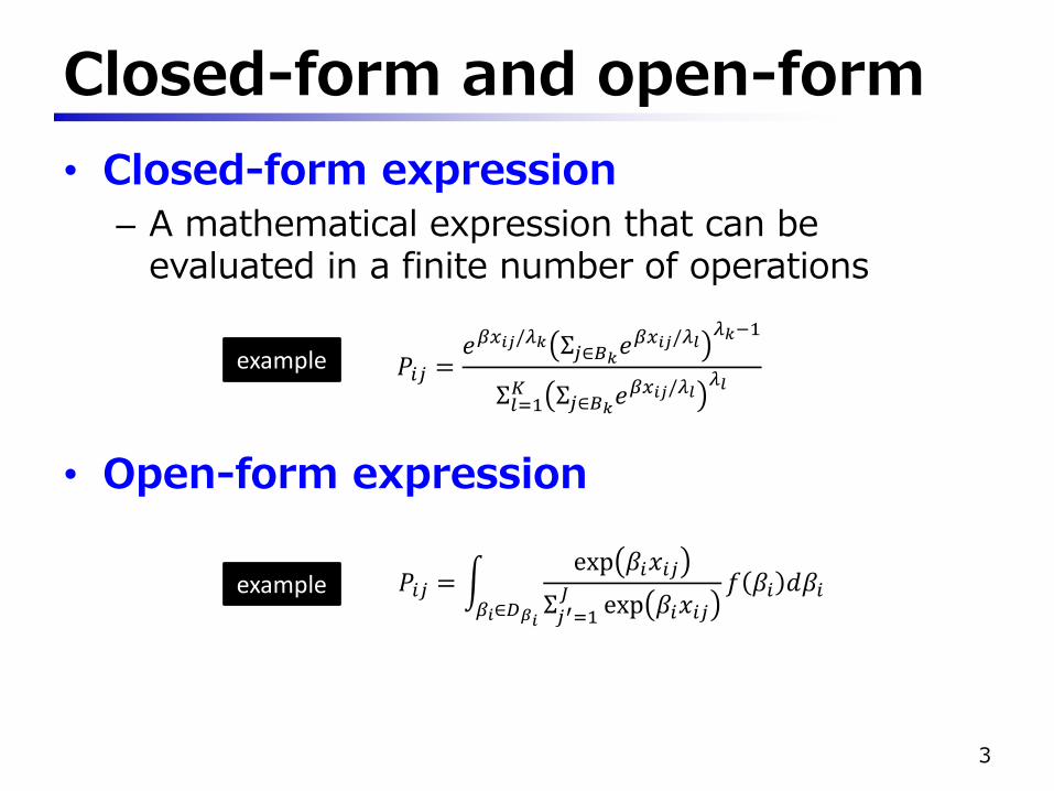
Closed-form and open-form

• Closed-form expression

– A mathematical expression that can be evaluated in a finite number of operations

• Open-form expression

3

𝑃𝑖𝑗 =𝑒𝛽𝑥𝑖𝑗/𝜆𝑘 Σ𝑗∈𝐵𝑘

𝑒𝛽𝑥𝑖𝑗/𝜆𝑙𝜆𝑘−1

Σ𝑙=1𝐾 Σ𝑗∈𝐵𝑘

𝑒𝛽𝑥𝑖𝑗/𝜆𝑙𝜆𝑙

example

𝑃𝑖𝑗 = 𝛽𝑖∈𝐷𝛽𝑖

exp 𝛽𝑖𝑥𝑖𝑗

Σ𝑗′=1𝐽 exp 𝛽𝑖𝑥𝑖𝑗

𝑓 𝛽𝑖 𝑑𝛽𝑖example

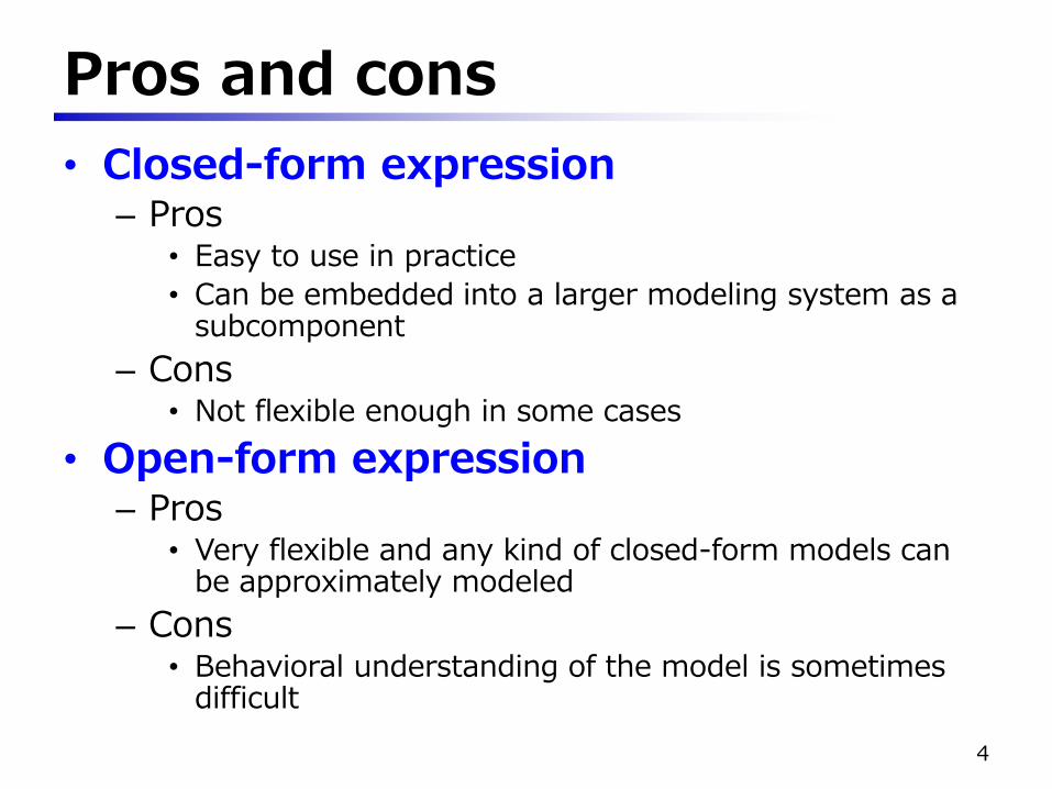
Pros and cons

• Closed-form expression– Pros

• Easy to use in practice

• Can be embedded into a larger modeling system as a subcomponent

– Cons• Not flexible enough in some cases

• Open-form expression– Pros

• Very flexible and any kind of closed-form models can be approximately modeled

– Cons• Behavioral understanding of the model is sometimes

difficult

4

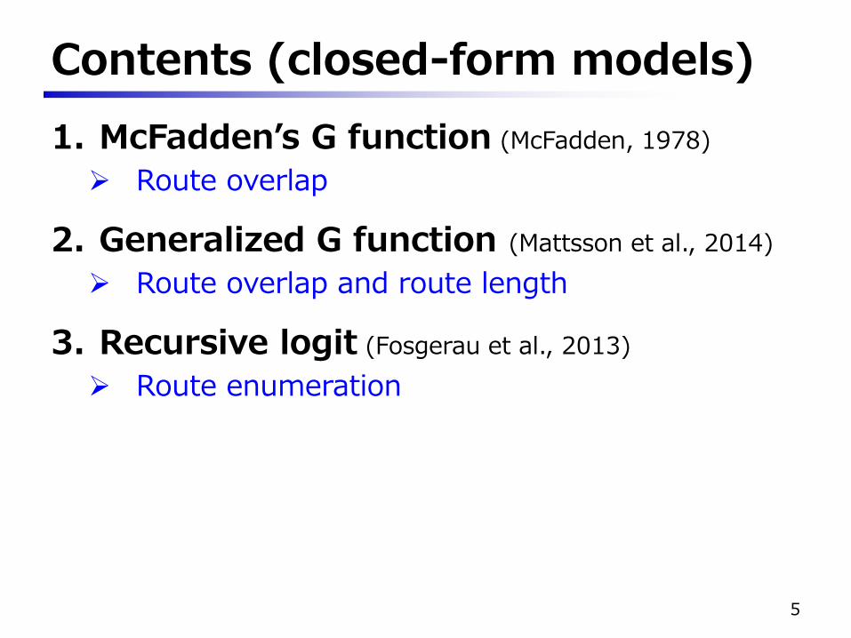
Contents (closed-form models)

1. McFadden’s G function (McFadden, 1978)

Route overlap

2. Generalized G function (Mattsson et al., 2014)

Route overlap and route length

3. Recursive logit (Fosgerau et al., 2013)

Route enumeration

5

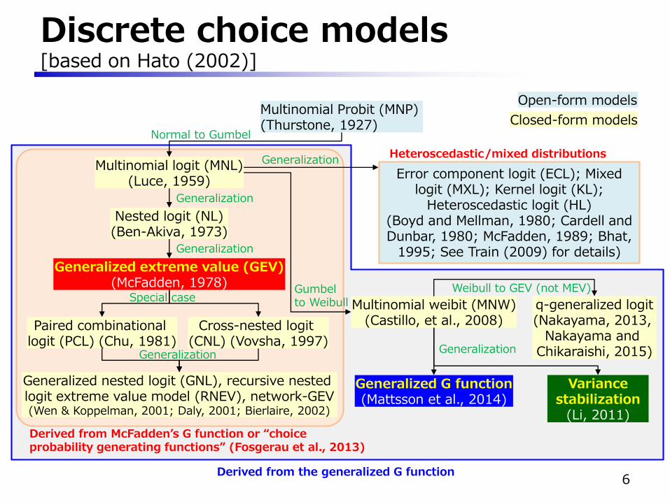
Discrete choice models[based on Hato (2002)]

6

Multinomial logit (MNL)(Luce, 1959)

Multinomial Probit (MNP)(Thurstone, 1927)

Nested logit (NL)(Ben-Akiva, 1973)

Generalized extreme value (GEV)(McFadden, 1978)

Paired combinational logit (PCL) (Chu, 1981)

Cross-nested logit (CNL) (Vovsha, 1997)

Generalized nested logit (GNL), recursive nested logit extreme value model (RNEV), network-GEV(Wen & Koppelman, 2001; Daly, 2001; Bierlaire, 2002)

Error component logit (ECL); Mixed logit (MXL); Kernel logit (KL);

Heteroscedastic logit (HL)(Boyd and Mellman, 1980; Cardell and Dunbar, 1980; McFadden, 1989; Bhat,

1995; See Train (2009) for details)

Normal to Gumbel

Generalization

Generalization

Generalization

Special case

Heteroscedastic/mixed distributions

Derived from McFadden’s G function or “choice probability generating functions” (Fosgerau et al., 2013)

Generalization

Multinomial weibit (MNW)(Castillo, et al., 2008)

Gumbel to Weibull q-generalized logit

(Nakayama, 2013, Nakayama and

Chikaraishi, 2015)

Variance stabilization

(Li, 2011)

Generalized G function(Mattsson et al., 2014)

Generalization

Derived from the generalized G function

Weibull to GEV (not MEV)

Closed-form models

Open-form models

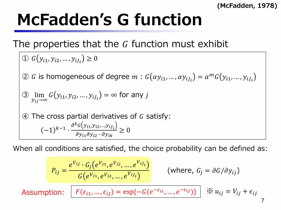
McFadden’s G function

7

The properties that the 𝐺 function must exhibit

① 𝐺 𝑦𝑖1, 𝑦𝑖2, … , 𝑦𝑖𝐽𝑖 ≥ 0

② 𝐺 is homogeneous of degree 𝑚：𝐺 𝛼𝑦𝑖1, … , 𝛼𝑦𝑖𝐽𝑖 = 𝛼𝑚𝐺 𝑦𝑖1, … , 𝑦𝑖𝐽𝑖

③ lim𝑦𝑖𝑗→∞

𝐺 𝑦𝑖1, 𝑦𝑖2, … , 𝑦𝑖𝐽𝑖 = ∞ for any 𝑗

④ The cross partial derivatives of 𝐺 satisfy:

−1 𝑘−1 ∙𝜕𝑘𝐺 𝑦𝑖1,𝑦𝑖2,…,𝑦𝑖𝐽𝑖

𝜕𝑦𝑖1𝜕𝑦𝑖2⋯𝜕𝑦𝑖𝑘≥ 0

When all conditions are satisfied, the choice probability can be defined as:

𝑃𝑖𝑗 =𝑒𝑉𝑖𝑗 ∙ 𝐺𝑗 𝑒𝑉𝑖1 , 𝑒𝑉𝑖2 , … , 𝑒𝑉𝑖𝐽𝑖

𝐺 𝑒𝑉𝑖1 , 𝑒𝑉𝑖2 , … , 𝑒𝑉𝑖𝐽𝑖

𝐹(𝜖𝑖1, … , 𝜖𝑖𝐽) = exp{−𝐺(𝑒−𝜖𝑖1 , … , 𝑒−𝜖𝑖𝐽)}Assumption:

(where, 𝐺𝑗 = 𝜕𝐺/𝜕𝑦𝑖𝑗)

(McFadden, 1978)

※ 𝑢𝑖𝑗 = 𝑉𝑖𝑗 + 𝜖𝑖𝑗

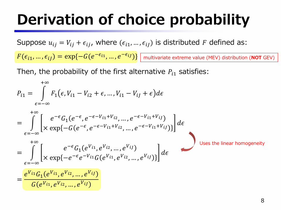
Derivation of choice probability

Suppose 𝑢𝑖𝑗 = 𝑉𝑖𝑗 + 𝜖𝑖𝑗, where (𝜖𝑖1, … , 𝜖𝑖𝐽) is distributed 𝐹 defined as:

𝐹(𝜖𝑖1, … , 𝜖𝑖𝐽) = exp{−𝐺(𝑒−𝜖𝑖1 , … , 𝑒−𝜖𝑖𝐽)}

Then, the probability of the first alternative 𝑃𝑖1 satisfies:

𝑃𝑖1 =

𝜖=−∞

+∞

𝐹1 𝜖, 𝑉𝑖1 − 𝑉𝑖2 + 𝜖,… , 𝑉𝑖1 − 𝑉𝑖𝐽 + 𝜖 𝑑𝜖

=

𝜖=−∞

+∞

𝑒−𝜖𝐺1 𝑒−𝜖, 𝑒−𝜖−𝑉𝑖1+𝑉𝑖2 , … , 𝑒−𝜖−𝑉𝑖1+𝑉𝑖𝐽

× exp −𝐺 𝑒−𝜖, 𝑒−𝜖−𝑉𝑖1+𝑉𝑖2 , … , 𝑒−𝜖−𝑉𝑖1+𝑉𝑖𝐽𝑑𝜖

=

𝜖=−∞

+∞

𝑒−𝜖𝐺1 𝑒𝑉𝑖1 , 𝑒𝑉𝑖2 , … , 𝑒𝑉𝑖𝐽

× exp −𝑒−𝜖𝑒−𝑉𝑖1𝐺 𝑒𝑉𝑖1 , 𝑒𝑉𝑖2 , … , 𝑒𝑉𝑖𝐽𝑑𝜖

=𝑒𝑉𝑖1𝐺1 𝑒𝑉𝑖1 , 𝑒𝑉𝑖2 , … , 𝑒𝑉𝑖𝐽

𝐺 𝑒𝑉𝑖1 , 𝑒𝑉𝑖2 , … , 𝑒𝑉𝑖𝐽

8

multivariate extreme value (MEV) distribution (NOT GEV)

Uses the linear homogeneity

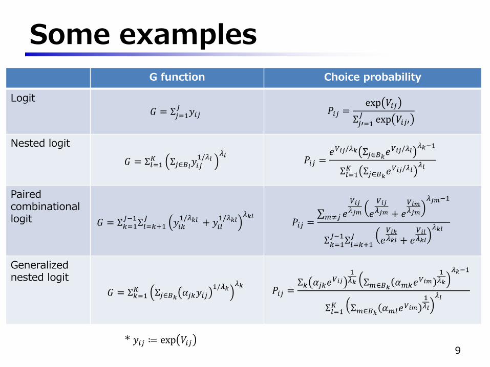
Some examples

G function Choice probability

Logit

𝐺 = Σ𝑗=1𝐽

𝑦𝑖𝑗 𝑃𝑖𝑗 =exp 𝑉𝑖𝑗

Σ𝑗′=1𝐽

exp 𝑉𝑖𝑗′

Nested logit

𝐺 = Σ𝑙=1𝐾 Σ𝑗∈𝐵𝑙

𝑦𝑖𝑗1/𝜆𝑙

𝜆𝑙𝑃𝑖𝑗 =

𝑒𝑉𝑖𝑗/𝜆𝑘 Σ𝑗∈𝐵𝑘𝑒𝑉𝑖𝑗/𝜆𝑙

𝜆𝑘−1

Σ𝑙=1𝐾 Σ𝑗∈𝐵𝑘

𝑒𝑉𝑖𝑗/𝜆𝑙𝜆𝑙

Pairedcombinational logit 𝐺 = Σ𝑘=1

𝐽−1Σ𝑙=𝑘+1𝐽

𝑦𝑖𝑘1/𝜆𝑘𝑙 + 𝑦𝑖𝑙

1/𝜆𝑘𝑙𝜆𝑘𝑙

𝑃𝑖𝑗 = 𝑚≠𝑗 𝑒

𝑉𝑖𝑗

𝜆𝑗𝑚 𝑒

𝑉𝑖𝑗

𝜆𝑗𝑚 + 𝑒𝑉𝑖𝑚𝜆𝑗𝑚

𝜆𝑗𝑚−1

Σ𝑘=1𝐽−1

Σ𝑙=𝑘+1𝐽

𝑒𝑉𝑖𝑘𝜆𝑘𝑙 + 𝑒

𝑉𝑖𝑙𝜆𝑘𝑙

𝜆𝑘𝑙

Generalized nested logit

𝐺 = Σ𝑘=1𝐾 Σ𝑗∈𝐵𝑘

𝛼𝑗𝑘𝑦𝑖𝑗1/𝜆𝑘

𝜆𝑘𝑃𝑖𝑗 =

Σ𝑘 𝛼𝑗𝑘𝑒𝑉𝑖𝑗

1𝜆𝑘 Σ𝑚∈𝐵𝑘

𝛼𝑚𝑘𝑒𝑉𝑖𝑚

1𝜆𝑘

𝜆𝑘−1

Σ𝑙=1𝐾 Σ𝑚∈𝐵𝑘

𝛼𝑚𝑙𝑒𝑉𝑖𝑚

1𝜆𝑙

𝜆𝑙

9* 𝑦𝑖𝑗 ≔ exp 𝑉𝑖𝑗

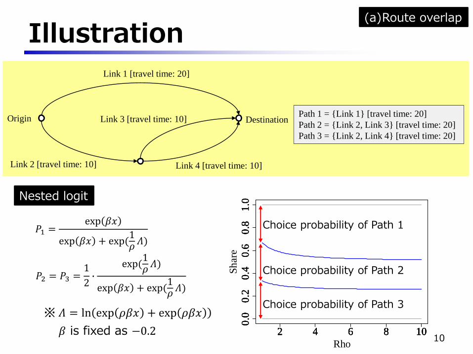
Illustration

10

Path 1 = {Link 1} [travel time: 20]

Path 2 = {Link 2, Link 3} [travel time: 20]

Path 3 = {Link 2, Link 4} [travel time: 20]

Origin Destination

Link 1 [travel time: 20]

Link 2 [travel time: 10] Link 4 [travel time: 10]

Link 3 [travel time: 10]

2 4 6 8 10

0.0

0.2

0.4

0.6

0.8

1.0

2 4 6 8 10

0.0

0.2

0.4

0.6

0.8

1.0

2 4 6 8 10

0.0

0.2

0.4

0.6

0.8

1.0

2 4 6 8 10

0.0

0.2

0.4

0.6

0.8

1.0

Rho

Sh

are

𝑃1 =exp 𝛽𝑥

exp 𝛽𝑥 + exp(1𝜌𝛬)

𝑃2 = 𝑃3 =1

2∙

exp(1𝜌𝛬)

exp 𝛽𝑥 + exp(1𝜌𝛬)

※ 𝛬 = ln exp 𝜌𝛽𝑥 + exp 𝜌𝛽𝑥

𝛽 is fixed as −0.2

Choice probability of Path 1

Choice probability of Path 3

Choice probability of Path 2

Nested logit

(a)Route overlap

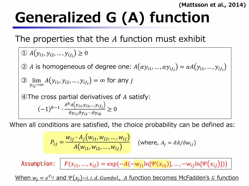
Generalized G (A) function

11

The properties that the 𝐴 function must exhibit

① 𝐴 𝑦𝑖1, 𝑦𝑖2, … , 𝑦𝑖𝐽𝑖 ≥ 0

② 𝐴 is homogeneous of degree one: 𝐴 𝛼𝑦𝑖1, … , 𝛼𝑦𝑖𝐽𝑖 = 𝛼𝐴 𝑦𝑖1, … , 𝑦𝑖𝐽𝑖

③ lim𝑦𝑖𝑗→∞

𝐴 𝑦𝑖1, 𝑦𝑖2, … , 𝑦𝑖𝐽𝑖 = ∞ for any 𝑗

④The cross partial derivatives of 𝐴 satisfy:

−1 𝑘−1 ∙𝜕𝑘𝐴 𝑦𝑖1,𝑦𝑖2,…,𝑦𝑖𝐽𝑖

𝜕𝑦𝑖1𝜕𝑦𝑖2⋯𝜕𝑦𝑖𝑘≥ 0

𝑃𝑖𝑗 =𝑤𝑖𝑗 ∙ 𝐴𝑗 𝑤𝑖1, 𝑤𝑖2, … , 𝑤𝑖𝐽

𝐴 𝑤𝑖1, 𝑤𝑖2, … , 𝑤𝑖𝐽

𝐹(𝑥𝑖1, … , 𝑥𝑖𝐽) = exp{−𝐴(−𝑤𝑖1ln[𝛹 𝑥𝑖1 ], … , −𝑤𝑖𝐽ln[𝛹 𝑥𝑖𝐽 ])}

When 𝑤𝑗 = 𝑒𝑉𝑖𝑗 and 𝛹 𝑥𝑗 ~𝑖. 𝑖. 𝑑. 𝐺𝑢𝑚𝑏𝑒𝑙, 𝐴 function becomes McFadden’s 𝐺 function

(Mattsson et al., 2014)

When all conditions are satisfied, the choice probability can be defined as:

(where, 𝐴𝑗 = 𝜕𝐴/𝜕𝑤𝑖𝑗)

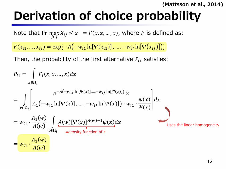
Derivation of choice probability

Note that Pr[max𝑗∈𝐽

𝑋𝑖𝑗 ≤ 𝑥] = 𝐹 𝑥, 𝑥, … , 𝑥 , where 𝐹 is defined as:

𝐹(𝑥𝑖1, … , 𝑥𝑖𝐽) = exp{−𝐴 −𝑤𝑖1 ln 𝛹 𝑥𝑖1 , … , −𝑤𝑖𝐽 ln 𝛹 𝑥𝑖𝐽 }

Then, the probability of the first alternative 𝑃𝑖1 satisfies:

𝑃𝑖1 =

𝑥∈Ω𝑖

𝐹1 𝑥, 𝑥, … , 𝑥 𝑑𝑥

=

𝑥∈Ω𝑖

𝑒−𝐴 −𝑤𝑖1 ln 𝛹 𝑥 ,…,−𝑤𝑖𝐽 ln 𝛹 𝑥 ×

𝐴1 −𝑤𝑖1 ln 𝛹 𝑥 ,… ,−𝑤𝑖𝐽 ln 𝛹 𝑥 ∙ 𝑤𝑖1 ∙𝜓 𝑥

𝛹 𝑥

𝑑𝑥

= 𝑤𝑖1 ∙𝐴1 𝑤

𝐴 𝑤

𝑥∈Ω𝑖

𝐴 𝑤 𝛹 𝑥 𝐴 𝑤 −1𝜓 𝑥 𝑑𝑥

= 𝑤𝑖1 ∙𝐴1 𝑤

𝐴 𝑤

12

Uses the linear homogeneity

=density function of 𝐹

(Mattsson et al., 2014)

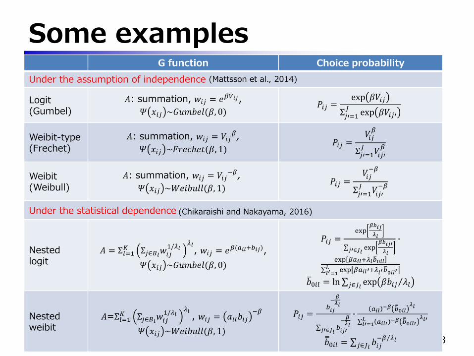
Some examples

13

G function Choice probability

Under the assumption of independence

Logit(Gumbel)

𝐴: summation, 𝑤𝑖𝑗 = 𝑒𝛽𝑉𝑖𝑗,

𝛹 𝑥𝑖𝑗 ~𝐺𝑢𝑚𝑏𝑒𝑙(𝛽, 0)𝑃𝑖𝑗 =

exp 𝛽𝑉𝑖𝑗

Σ𝑗′=1𝐽

exp 𝛽𝑉𝑖𝑗′

Weibit-type(Frechet)

𝐴: summation, 𝑤𝑖𝑗 = 𝑉𝑖𝑗𝛽,

𝛹 𝑥𝑖𝑗 ~𝐹𝑟𝑒𝑐ℎ𝑒𝑡(𝛽, 1)𝑃𝑖𝑗 =

𝑉𝑖𝑗𝛽

Σ𝑗′=1𝐽

𝑉𝑖𝑗′𝛽

Weibit(Weibull)

𝐴: summation, 𝑤𝑖𝑗 = 𝑉𝑖𝑗−𝛽,

𝛹 𝑥𝑖𝑗 ~𝑊𝑒𝑖𝑏𝑢𝑙𝑙(𝛽, 1)𝑃𝑖𝑗 =

𝑉𝑖𝑗−𝛽

Σ𝑗′=1𝐽

𝑉𝑖𝑗′−𝛽

Under the statistical dependence

Nestedlogit

𝐴 = Σ𝑙=1𝐾 Σ𝑗∈𝐵𝑙

𝑤𝑖𝑗1/𝜆𝑙

𝜆𝑙, 𝑤𝑖𝑗 = 𝑒𝛽(𝑎𝑖𝑙+𝑏𝑖𝑗),

𝛹 𝑥𝑖𝑗 ~𝐺𝑢𝑚𝑏𝑒𝑙(𝛽, 0)

𝑃𝑖𝑗 =exp

𝛽𝑏𝑖𝑗

𝜆𝑙

𝑗′∈𝐽𝑙exp

𝛽𝑏𝑖𝑗′

𝜆𝑙

∙

exp 𝛽𝑎𝑖𝑙+𝜆𝑙 𝑏0𝑖𝑙

𝑙′=1𝐿 exp 𝛽𝑎𝑖𝑙′+𝜆𝑙′

𝑏0𝑖𝑙′

𝑏0𝑖𝑙 = ln 𝑗∈𝐽𝑙exp 𝛽𝑏𝑖𝑗 𝜆𝑙

Nested weibit

𝐴=Σ𝑙=1𝐾 Σ𝑗∈𝐵𝑙

𝑤𝑖𝑗1/𝜆𝑙

𝜆𝑙, 𝑤𝑖𝑗 = 𝑎𝑖𝑙𝑏𝑖𝑗

−𝛽

𝛹 𝑥𝑖𝑗 ~𝑊𝑒𝑖𝑏𝑢𝑙𝑙(𝛽, 1)

𝑃𝑖𝑗 =𝑏𝑖𝑗

−𝛽𝜆𝑙

𝑗′∈𝐽𝑙𝑏𝑖𝑗′

−𝛽𝜆𝑙

∙𝑎𝑖𝑙

−𝛽 𝑏0𝑖𝑙𝜆𝑙

𝑙′=1𝐿 𝑎𝑖𝑙′

−𝛽 𝑏0𝑖𝑙′𝜆𝑙′

𝑏0𝑖𝑙 = 𝑗∈𝐽𝑙𝑏𝑖𝑗− 𝛽 𝜆𝑙

(Mattsson et al., 2014)

(Chikaraishi and Nakayama, 2016)

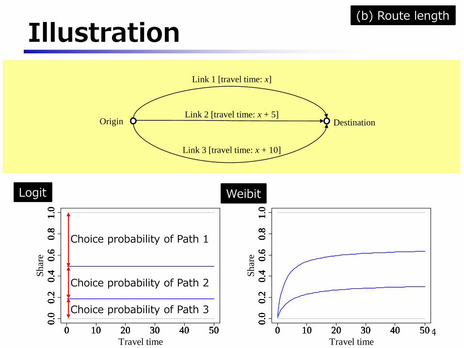
Illustration

14

Origin Destination

Link 1 [travel time: x]

Link 2 [travel time: x + 5]

Link 3 [travel time: x + 10]

Logit Weibit

0 10 20 30 40 50

0.0

0.2

0.4

0.6

0.8

1.0

0 10 20 30 40 50

0.0

0.2

0.4

0.6

0.8

1.0

0 10 20 30 40 50

0.0

0.2

0.4

0.6

0.8

1.0

0 10 20 30 40 50

0.0

0.2

0.4

0.6

0.8

1.0

Travel time

Sh

are

0 10 20 30 40 50

0.0

0.2

0.4

0.6

0.8

1.0

0 10 20 30 40 50

0.0

0.2

0.4

0.6

0.8

1.0

0 10 20 30 40 50

0.0

0.2

0.4

0.6

0.8

1.0

0 10 20 30 40 50

0.0

0.2

0.4

0.6

0.8

1.0

Travel time

Sh

are

Choice probability of Path 1

Choice probability of Path 3

Choice probability of Path 2

(b) Route length

0 10 20 30 40 50

0.0

0.2

0.4

0.6

0.8

1.0

0 10 20 30 40 50

0.0

0.2

0.4

0.6

0.8

1.0

0 10 20 30 40 50

0.0

0.2

0.4

0.6

0.8

1.0

0 10 20 30 40 50

0.0

0.2

0.4

0.6

0.8

1.0

0 10 20 30 40 50

0.0

0.2

0.4

0.6

0.8

1.0

0 10 20 30 40 50

0.0

0.2

0.4

0.6

0.8

1.0

0 10 20 30 40 50

0.0

0.2

0.4

0.6

0.8

1.0

0 10 20 30 40 50

0.0

0.2

0.4

0.6

0.8

1.0

Travel time

Sh

are

0 10 20 30 40 50

0.0

0.2

0.4

0.6

0.8

1.0

0 10 20 30 40 50

0.0

0.2

0.4

0.6

0.8

1.0

0 10 20 30 40 50

0.0

0.2

0.4

0.6

0.8

1.0

0 10 20 30 40 50

0.0

0.2

0.4

0.6

0.8

1.0

0 10 20 30 40 50

0.0

0.2

0.4

0.6

0.8

1.0

0 10 20 30 40 50

0.0

0.2

0.4

0.6

0.8

1.0

0 10 20 30 40 50

0.0

0.2

0.4

0.6

0.8

1.0

0 10 20 30 40 50

0.0

0.2

0.4

0.6

0.8

1.0

Travel time

Sh

are

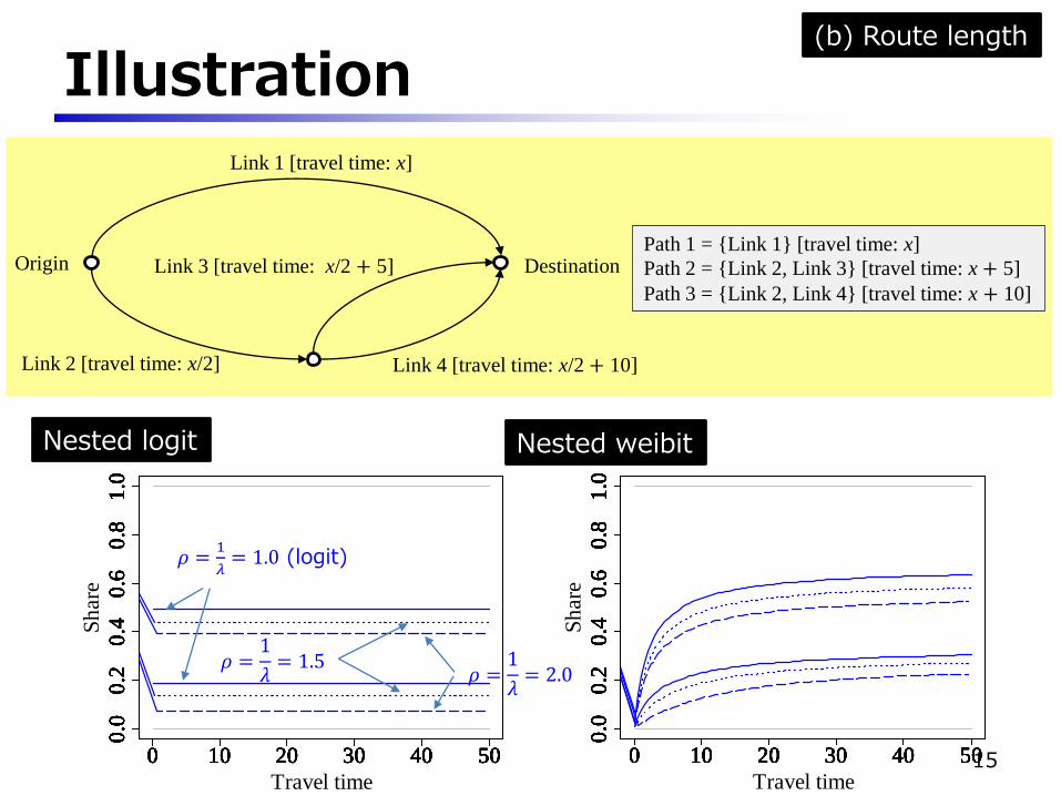
Illustration

15

Nested logit Nested weibit

Origin Destination

Link 1 [travel time: x]

Link 2 [travel time: x/2] Link 4 [travel time: x/2 + 10]

Link 3 [travel time: x/2 + 5]Path 1 = {Link 1} [travel time: x]

Path 2 = {Link 2, Link 3} [travel time: x + 5]

Path 3 = {Link 2, Link 4} [travel time: x + 10]

𝜌 =1

𝜆= 1.0 (logit)

𝜌 =1

𝜆= 1.5

𝜌 =1

𝜆= 2.0

(b) Route length

Recursive logit

16

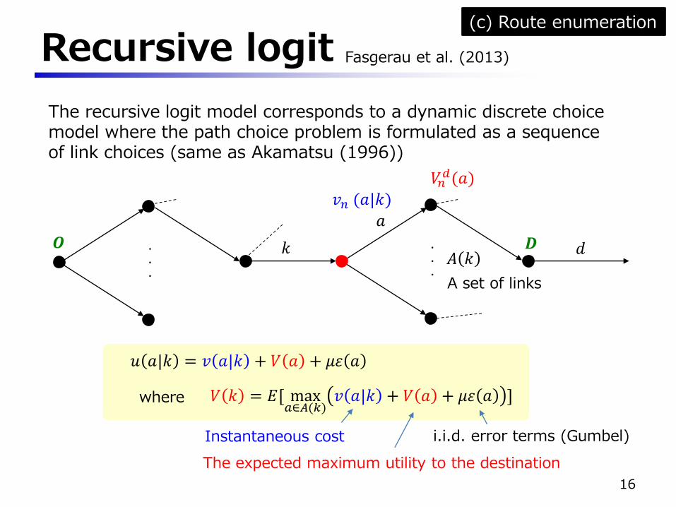
The recursive logit model corresponds to a dynamic discrete choice model where the path choice problem is formulated as a sequence of link choices (same as Akamatsu (1996))

Fasgerau et al. (2013)

𝑢 𝑎|𝑘 = 𝑣 𝑎|𝑘 + 𝑉 𝑎 + 𝜇𝜀 𝑎

𝑉 𝑘 = 𝐸[ max𝑎∈𝐴(𝑘)

𝑣 𝑎|𝑘 + 𝑉 𝑎 + 𝜇𝜀 𝑎 ]where

𝑉𝑛𝑑(𝑎)

𝑑𝑘

𝑎

𝑫𝑶 ...

.

.

.𝐴 𝑘

A set of links

𝑣𝑛 (𝑎|𝑘)

Instantaneous cost

The expected maximum utility to the destination

i.i.d. error terms (Gumbel)

(c) Route enumeration

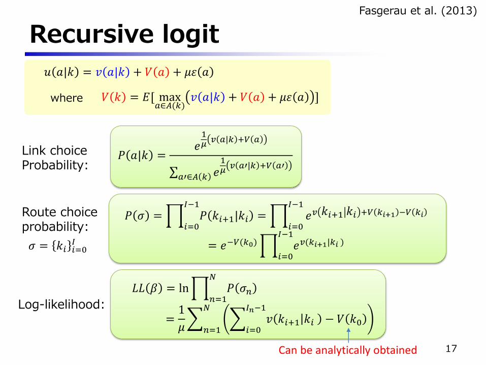
Recursive logit

17

𝑃 𝑎|𝑘 =𝑒1𝜇 𝑣 𝑎|𝑘 +𝑉 𝑎

𝑎′∈𝐴 𝑘 𝑒1𝜇 𝑣 𝑎′|𝑘 +𝑉 𝑎′

𝑃 𝜎 = 𝑖=0

𝐼−1

𝑃 𝑘𝑖+1|𝑘𝑖 = 𝑖=0

𝐼−1

𝑒𝑣 𝑘𝑖+1 𝑘𝑖 +𝑉 𝑘𝑖+1 −𝑉 𝑘𝑖

= 𝑒−𝑉(𝑘0) 𝑖=0

𝐼−1

𝑒𝑣(𝑘𝑖+1|𝑘𝑖 )

Link choiceProbability:

Route choice probability:

𝜎 = 𝑘𝑖 𝑖=0𝐼

Fasgerau et al. (2013)

𝑢 𝑎|𝑘 = 𝑣 𝑎|𝑘 + 𝑉 𝑎 + 𝜇𝜀 𝑎

𝑉 𝑘 = 𝐸[ max𝑎∈𝐴(𝑘)

𝑣 𝑎|𝑘 + 𝑉 𝑎 + 𝜇𝜀 𝑎 ]where

𝐿𝐿 𝛽 = ln 𝑛=1

𝑁

𝑃 𝜎𝑛

=1

𝜇

𝑛=1

𝑁

𝑖=0

𝐼𝑛−1

𝑣 𝑘𝑖+1 𝑘𝑖 − 𝑉 𝑘0

Log-likelihood:

Can be analytically obtained

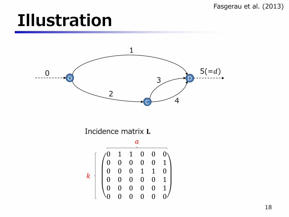
Illustration

18

O D

C

5(=𝑑)

1

2

3

4

Incidence matrix 𝐋

0 1 1 0 0 00 0 0 0 0 10 0 0 1 1 00 0 0 0 0 10 0 0 0 0 10 0 0 0 0 0

0

𝑘

𝑎

Fasgerau et al. (2013)

19

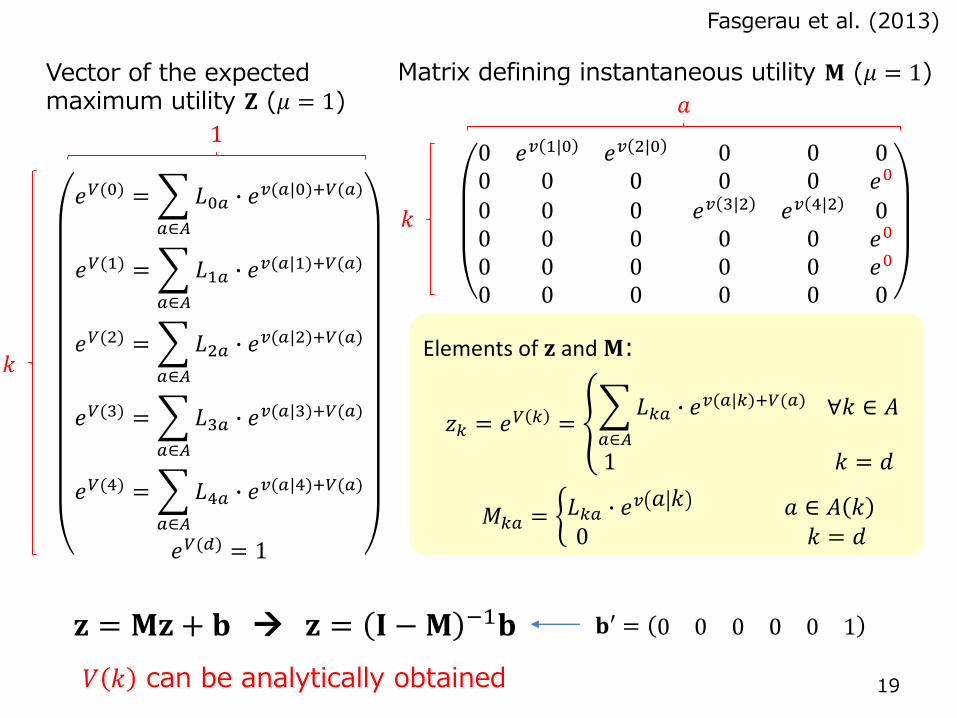
Vector of the expectedmaximum utility 𝐙 (𝜇 = 1)

𝑒𝑉(0) =

𝑎∈𝐴

𝐿0𝑎 ∙ 𝑒𝑣(𝑎|0)+𝑉(𝑎)

𝑒𝑉(1) =

𝑎∈𝐴

𝐿1𝑎 ∙ 𝑒𝑣(𝑎|1)+𝑉(𝑎)

𝑒𝑉(2) =

𝑎∈𝐴

𝐿2𝑎 ∙ 𝑒𝑣(𝑎|2)+𝑉(𝑎)

𝑒𝑉(3) =

𝑎∈𝐴

𝐿3𝑎 ∙ 𝑒𝑣(𝑎|3)+𝑉(𝑎)

𝑒𝑉(4) =

𝑎∈𝐴

𝐿4𝑎 ∙ 𝑒𝑣(𝑎|4)+𝑉(𝑎)

𝑒𝑉(𝑑) = 1

𝑘

1

Matrix defining instantaneous utility 𝐌 (𝜇 = 1)

0 𝑒𝑣 1|0 𝑒𝑣 2|0 0 0 00 0 0 0 0 𝑒0

0 0 0 𝑒𝑣 3|2 𝑒𝑣 4|2 00 0 0 0 0 𝑒0

0 0 0 0 0 𝑒0

0 0 0 0 0 0

𝑘

𝑎

Elements of 𝐳 and 𝐌:

𝑧𝑘 = 𝑒𝑉 𝑘 =

𝑎∈𝐴

𝐿𝑘𝑎 ∙ 𝑒𝑣(𝑎|𝑘)+𝑉(𝑎) ∀𝑘 ∈ 𝐴

1 𝑘 = 𝑑

𝑀𝑘𝑎 = 𝐿𝑘𝑎 ∙ 𝑒𝑣 𝑎 𝑘 𝑎 ∈ 𝐴 𝑘0 𝑘 = 𝑑

Fasgerau et al. (2013)

𝐳 = 𝐌𝐳 + 𝐛 𝐳 = 𝐈 −𝐌 −1𝐛 𝐛′ = 0 0 0 0 0 1

𝑉 𝑘 can be analytically obtained

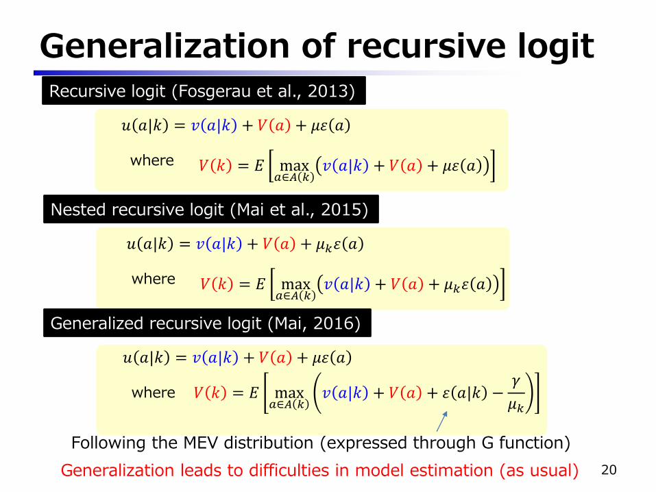
Generalization of recursive logit

20

𝑢 𝑎|𝑘 = 𝑣 𝑎|𝑘 + 𝑉 𝑎 + 𝜇𝜀 𝑎

𝑉 𝑘 = 𝐸 max𝑎∈𝐴 𝑘

𝑣 𝑎|𝑘 + 𝑉 𝑎 + 𝜇𝜀 𝑎where

Recursive logit (Fosgerau et al., 2013)

𝑢 𝑎|𝑘 = 𝑣 𝑎|𝑘 + 𝑉 𝑎 + 𝜇𝑘𝜀 𝑎

𝑉 𝑘 = 𝐸 max𝑎∈𝐴 𝑘

𝑣 𝑎|𝑘 + 𝑉 𝑎 + 𝜇𝑘𝜀 𝑎where

Nested recursive logit (Mai et al., 2015)

𝑢 𝑎|𝑘 = 𝑣 𝑎|𝑘 + 𝑉 𝑎 + 𝜇𝜀 𝑎

𝑉 𝑘 = 𝐸 max𝑎∈𝐴 𝑘

𝑣 𝑎|𝑘 + 𝑉 𝑎 + 𝜀 𝑎|𝑘 −𝛾

𝜇𝑘where

Generalized recursive logit (Mai, 2016)

Following the MEV distribution (expressed through G function)

Generalization leads to difficulties in model estimation (as usual)

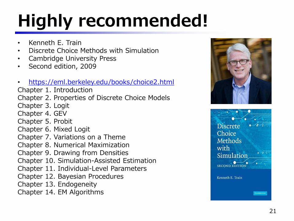
Highly recommended!• Kenneth E. Train• Discrete Choice Methods with Simulation• Cambridge University Press• Second edition, 2009

• https://eml.berkeley.edu/books/choice2.htmlChapter 1. IntroductionChapter 2. Properties of Discrete Choice ModelsChapter 3. LogitChapter 4. GEVChapter 5. ProbitChapter 6. Mixed LogitChapter 7. Variations on a ThemeChapter 8. Numerical MaximizationChapter 9. Drawing from DensitiesChapter 10. Simulation-Assisted EstimationChapter 11. Individual-Level ParametersChapter 12. Bayesian ProceduresChapter 13. EndogeneityChapter 14. EM Algorithms

21

References• Ben-Akiva, M. (1973) Structure of passenger travel demand models. Ph.D. Thesis,

Massachusetts Institute of Technology. Dept. of Civil and Environmental Engineering (http://hdl.handle.net/1721.1/14790 ).

• Bhat, C.R. (1995) A heteroscedastic extreme value model of intercity travel mode choice. Transportation Research Part B 29, 471-483.

• Bierlaire, M. (2002) The Network GEV model. Proceedings of the 2nd Swiss Transportation Research Conference, Ascona, Switzerland.

• Cardell, N.S., Dunbar, F.C. (1980) Measuring the societal impacts of automobile downsizing. Transportation Research Part A: General 14, 423-434.

• Castillo, E., Menendez, J.M., Jimenez, P., Rivas, A. (2008) Closed form expressions for choice probabilities in the Weibull case. Transportation Research Part B 42, 373-380.

• Chikaraishi, M., Nakayama, S. (2016) Discrete choice models with q-product random utilities, Transportation Research Part B (forthcoming).

• Daly, A. (2001) Recursive nested EV model. ITS Working Paper 559, Institute for Transport Studies, University of Leeds.

• Daly, A., Bierlaire, M. (2006) A general and operational representation of Generalised Extreme Value models. Transportation Research Part B: Methodological 40, 285-305.

22

References• Fosgerau, M., McFadden, D., Bierlaire, M. (2013) Choice probability generating

functions. Journal of Choice Modelling 8, 1-18.

• Fosgerau, M., Frejinger, E., Karlstrom, A., 2013. A link based network route choice model with unrestricted choice set. Transportation Research Part B: Methodological 56, 70-80.

• Hato, E. (2002) Behaviors in network, Infrastructure Planning Review, 19-1, 13-27 (in Japanese).

• Koppelman, F.S., Wen, C.-H. (2000) The paired combinatorial logit model: properties, estimation and application. Transportation Research Part B: Methodological 34, 75-89.

• Li, B. (2011) The multinomial logit model revisited: A semi-parametric approach in discrete choice analysis. Transportation Research Part B 45, 461-473.

• Luce, R. (1959) Individual Choice Beahviour. John Wiley, New York.

• Mai, T., Fosgerau, M., Frejinger, E., 2015. A nested recursive logit model for route choice analysis. Transportation Research Part B: Methodological 75, 100-112.

• Mai, T., 2016. A method of integrating correlation structures for a generalized recursive route choice model. Transportation Research Part B: Methodological 93, Part A, 146-161.

• Mattsson, L.-G., Weibull, J.W., Lindberg, P.O. (2014) Extreme values, invariance and choice probabilities. Transportation Research Part B: Methodological 59, 81-95.

23

References• McFadden, D., (1978) Modelling the choice of residential location, in: Karlqvist, A.,

Lundqvist, L., Snickars, F., Weibull, J. (Eds.), Spatial Interaction Theory and Residential Location. North-Holland, Amsterdam.

• McFadden, D. (1989) A Method of Simulated Moments for Estimation of Discrete Response Models Without Numerical Integration. Econometrica 57, 995-1026.

• Nakayama, S. (2013) q-generalized logit route choice and network equilibrium model. Proceedings of the 20th International Symposium on Transportation and Traffic Theory (Poster Session).

• Nakayama, S., Chikaraishi, M., 2015. Unified closed-form expression of logit and weibit and its extension to a transportation network equilibrium assignment. Transportation Research Part B 81, 672-685.

• Thurstone, L.L. (1927) A law of comparative judgment. Psychological Review 34, 273-286.

• Train, K. (2009) Discrete Choice Methods with Simulation, 2nd Edition ed. Cambridge University Press.

• Vovsha, P. (1997) Cross-nested logit model: an application to mode choice in the Tel-Aviv metropolitan area. Transportation Research Board, Presented at the 76th Annual Meeting, Washington DC.

• Wen, C.-H., Koppelman, F.S. (2001) The generalized nested logit model. Transportation Research Part B 35, 627-641.

24