RECENT DEVELOPMENTS IN LARGE DIMENSIONAL FACTOR …
151
RECENT DEVELOPMENTS IN LARGE DIMENSIONAL FACTOR ANALYSIS Serena Ng June 2007 SCE Meeting, Montreal Serena Ng () RECENT DEVELOPMENTS IN LARGE DIMENSIONAL FACTOR ANALYSIS June 2007 SCE Meeting, Montreal 1/ 58
Transcript of RECENT DEVELOPMENTS IN LARGE DIMENSIONAL FACTOR …
RECENT DEVELOPMENTS IN LARGEDIMENSIONAL FACTOR ANALYSIS
Serena Ng
June 2007SCE Meeting, Montreal
Serena Ng () RECENT DEVELOPMENTS IN LARGE DIMENSIONAL FACTOR ANALYSISJune 2007 SCE Meeting, Montreal 1 /
58
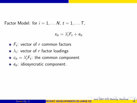
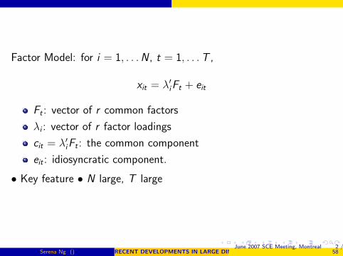
Factor Model: for i = 1, . . .N , t = 1, . . .T ,
xit = λ′iFt + eit
Ft : vector of r common factors
λi : vector of r factor loadings
cit = λ′iFt : the common component
eit : idiosyncratic component.
• Key feature • N large, T large
Serena Ng () RECENT DEVELOPMENTS IN LARGE DIMENSIONAL FACTOR ANALYSISJune 2007 SCE Meeting, Montreal 2 /
58
Outline of the talk
Applications of factor models
Sketch econometric framework
Main Statistical results
Caveats, theory and practice
What next?
Serena Ng () RECENT DEVELOPMENTS IN LARGE DIMENSIONAL FACTOR ANALYSISJune 2007 SCE Meeting, Montreal 3 /
58
Outline of the talk
Applications of factor models
Sketch econometric framework
Main Statistical results
Caveats, theory and practice
What next?
Serena Ng () RECENT DEVELOPMENTS IN LARGE DIMENSIONAL FACTOR ANALYSISJune 2007 SCE Meeting, Montreal 3 /
58
Outline of the talk
Applications of factor models
Sketch econometric framework
Main Statistical results
Caveats, theory and practice
What next?
Serena Ng () RECENT DEVELOPMENTS IN LARGE DIMENSIONAL FACTOR ANALYSISJune 2007 SCE Meeting, Montreal 3 /
58
Outline of the talk
Applications of factor models
Sketch econometric framework
Main Statistical results
Caveats, theory and practice
What next?
Serena Ng () RECENT DEVELOPMENTS IN LARGE DIMENSIONAL FACTOR ANALYSISJune 2007 SCE Meeting, Montreal 3 /
58
Outline of the talk
Applications of factor models
Sketch econometric framework
Main Statistical results
Caveats, theory and practice
What next?
Serena Ng () RECENT DEVELOPMENTS IN LARGE DIMENSIONAL FACTOR ANALYSISJune 2007 SCE Meeting, Montreal 3 /
58

Contributors to the Literature
T.W. Anderson, Lawley and Maxwell, ....;
Chris Sims, John Geweke, Tom Sargent, Danny Quah;
George Connor, George Korajczyk
Gary Chamerlain, Michael Rothschild
Jushan Bai, Jim Stock, Mark Watson;
Lucrezia Reichlin, Marco Lippi, Mario Forni, Marc Hallin;
Domenico Giannone, Catherine Doz
Jean Boivn, Marc Giannoni
Fashid Vahid, Heather Robertson, Roger Moon, Benoit Perron;
Alexei Ontaski, Matt Harding.
Serena Ng () RECENT DEVELOPMENTS IN LARGE DIMENSIONAL FACTOR ANALYSISJune 2007 SCE Meeting, Montreal 4 /
58
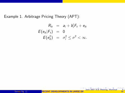
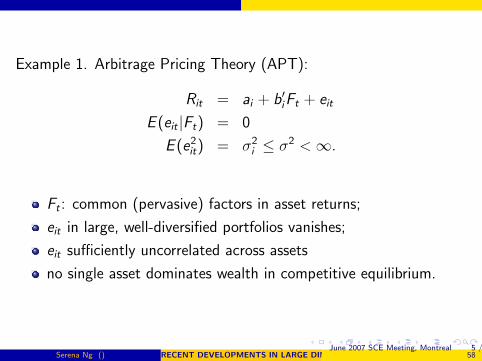
Example 1. Arbitrage Pricing Theory (APT):
Rit = ai + b′iFt + eit
E (eit |Ft) = 0
E (e2it) = σ2
i ≤ σ2 <∞.
Ft : common (pervasive) factors in asset returns;
eit in large, well-diversified portfolios vanishes;
eit sufficiently uncorrelated across assets
no single asset dominates wealth in competitive equilibrium.
Serena Ng () RECENT DEVELOPMENTS IN LARGE DIMENSIONAL FACTOR ANALYSISJune 2007 SCE Meeting, Montreal 5 /
58
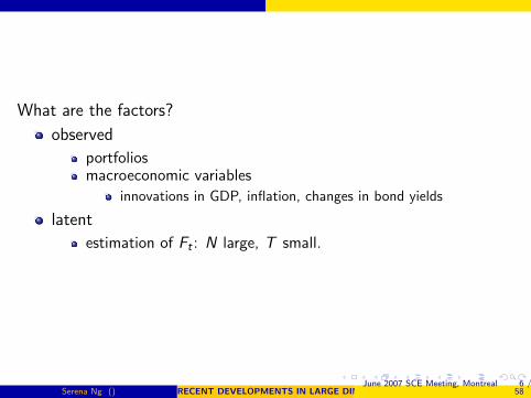
What are the factors?
observed
portfoliosmacroeconomic variables
innovations in GDP, inflation, changes in bond yields
latent
estimation of Ft : N large, T small.
Serena Ng () RECENT DEVELOPMENTS IN LARGE DIMENSIONAL FACTOR ANALYSISJune 2007 SCE Meeting, Montreal 6 /
58
What are the factors?
observed
portfoliosmacroeconomic variables
innovations in GDP, inflation, changes in bond yields
latent
estimation of Ft : N large, T small.
Serena Ng () RECENT DEVELOPMENTS IN LARGE DIMENSIONAL FACTOR ANALYSISJune 2007 SCE Meeting, Montreal 6 /
58
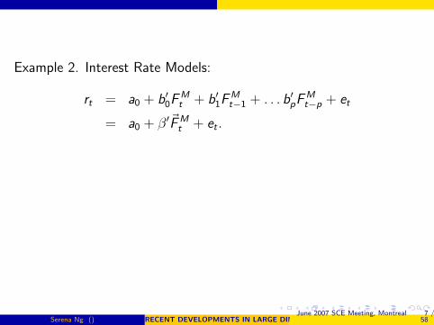
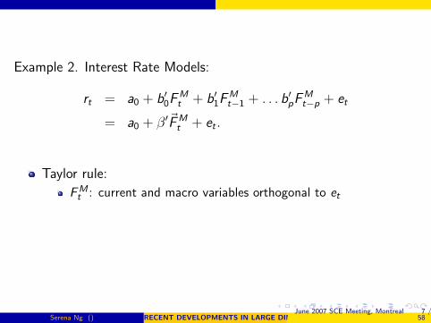
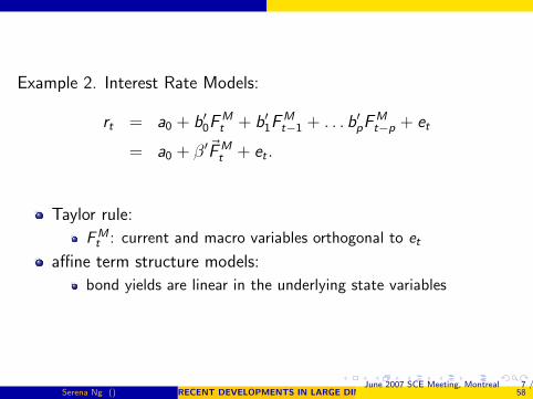
Example 2. Interest Rate Models:
rt = a0 + b′0FMt + b′1F
Mt−1 + . . . b′pF
Mt−p + et
= a0 + β′~FMt + et .
Taylor rule:
FMt : current and macro variables orthogonal to et
affine term structure models:
bond yields are linear in the underlying state variables
Serena Ng () RECENT DEVELOPMENTS IN LARGE DIMENSIONAL FACTOR ANALYSISJune 2007 SCE Meeting, Montreal 7 /
58
Example 3. Demand Systems: J goods, H households
Eh = total spending on J goods by household h;
Marshallian demand: Xjh = gj(p,Eh)
budget share: wjh = Xjh/Eh
the rank of a demand system holding prices fixed
the smallest integer r such that
wj(E ) = λj1G1(E ) + . . . λjrGr (E ).
Fh = (G1(Eh), . . .Gr (Eh))′ are r factors across goods
Serena Ng () RECENT DEVELOPMENTS IN LARGE DIMENSIONAL FACTOR ANALYSISJune 2007 SCE Meeting, Montreal 8 /
58
Example 4. Coincident index
y1t = λ1Ft + z1t
y2t = λ2Ft + z2t
y3t = λ3Ft + z3t
y4t = λ4Ft + z4t
Ft = φFt−1 + vt
zit = αizit−1 + eit , i = 1, . . . 4.
N = 4, T large.
Serena Ng () RECENT DEVELOPMENTS IN LARGE DIMENSIONAL FACTOR ANALYSISJune 2007 SCE Meeting, Montreal 9 /
58
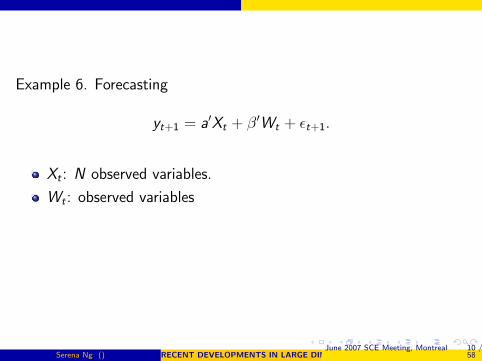
Example 6. Forecasting
yt+1 = a′Xt + β′Wt + εt+1.
Xt : N observed variables.
Wt : observed variables
N large: inefficient
Assume Xit have common sources of variation Ft .
Serena Ng () RECENT DEVELOPMENTS IN LARGE DIMENSIONAL FACTOR ANALYSISJune 2007 SCE Meeting, Montreal 10 /
58
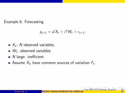
Example 6. Forecasting
yt+1 = a′Xt + β′Wt + εt+1.
Xt : N observed variables.
Wt : observed variables
N large: inefficient
Assume Xit have common sources of variation Ft .
Serena Ng () RECENT DEVELOPMENTS IN LARGE DIMENSIONAL FACTOR ANALYSISJune 2007 SCE Meeting, Montreal 10 /
58
Example 6. Forecasting
yt+1 = a′Xt + β′Wt + εt+1.
Xt : N observed variables.
Wt : observed variables
N large: inefficient
Assume Xit have common sources of variation Ft .
Serena Ng () RECENT DEVELOPMENTS IN LARGE DIMENSIONAL FACTOR ANALYSISJune 2007 SCE Meeting, Montreal 10 /
58
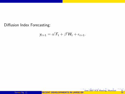
Diffusion Index Forecasting:
yt+1 = α′Ft + β′Wt + εt+1.
eg: Fed reacts to state of the economy.
rt = α′Ft + εt .
Serena Ng () RECENT DEVELOPMENTS IN LARGE DIMENSIONAL FACTOR ANALYSISJune 2007 SCE Meeting, Montreal 11 /
58
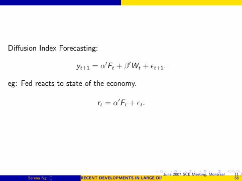
Diffusion Index Forecasting:
yt+1 = α′Ft + β′Wt + εt+1.
eg: Fed reacts to state of the economy.
rt = α′Ft + εt .
Serena Ng () RECENT DEVELOPMENTS IN LARGE DIMENSIONAL FACTOR ANALYSISJune 2007 SCE Meeting, Montreal 11 /
58
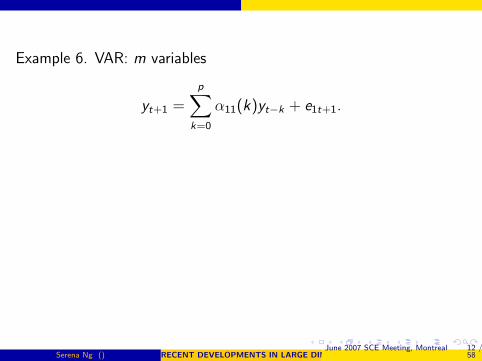
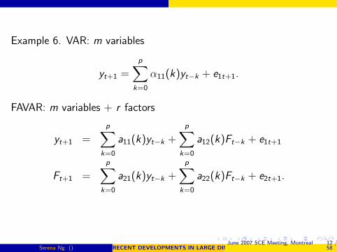
Example 6. VAR: m variables
yt+1 =
p∑k=0
α11(k)yt−k + e1t+1.
FAVAR: m variables + r factors
yt+1 =
p∑k=0
a11(k)yt−k +
p∑k=0
a12(k)Ft−k + e1t+1
Ft+1 =
p∑k=0
a21(k)yt−k +
p∑k=0
a22(k)Ft−k + e2t+1.
Serena Ng () RECENT DEVELOPMENTS IN LARGE DIMENSIONAL FACTOR ANALYSISJune 2007 SCE Meeting, Montreal 12 /
58
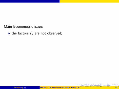
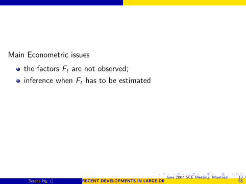
Main Econometric issues
the factors Ft are not observed;
inference when Ft has to be estimated
the number of factors r is unknown
N and T both large
Serena Ng () RECENT DEVELOPMENTS IN LARGE DIMENSIONAL FACTOR ANALYSISJune 2007 SCE Meeting, Montreal 13 /
58
Main Econometric issues
the factors Ft are not observed;
inference when Ft has to be estimated
the number of factors r is unknown
N and T both large
Serena Ng () RECENT DEVELOPMENTS IN LARGE DIMENSIONAL FACTOR ANALYSISJune 2007 SCE Meeting, Montreal 13 /
58
Main Econometric issues
the factors Ft are not observed;
inference when Ft has to be estimated
the number of factors r is unknown
N and T both large
Serena Ng () RECENT DEVELOPMENTS IN LARGE DIMENSIONAL FACTOR ANALYSISJune 2007 SCE Meeting, Montreal 13 /
58
Main Econometric issues
the factors Ft are not observed;
inference when Ft has to be estimated
the number of factors r is unknown
N and T both large
Serena Ng () RECENT DEVELOPMENTS IN LARGE DIMENSIONAL FACTOR ANALYSISJune 2007 SCE Meeting, Montreal 13 /
58
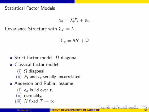
Statistical Factor Models
xit = λ′iFt + eit .
Covariance Structure with ΣF = Ir .
Σx = ΛΛ′ + Ω
Strict factor model: Ω diagonal
Classical factor model:
(i) Ω diagonal(ii) Ft and et serially uncorrelated
Anderson and Rubin: assume
(i) eit is iid over t,(ii) normality,(iii) N fixed T →∞.
Serena Ng () RECENT DEVELOPMENTS IN LARGE DIMENSIONAL FACTOR ANALYSISJune 2007 SCE Meeting, Montreal 14 /
58
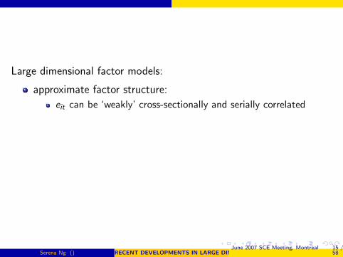
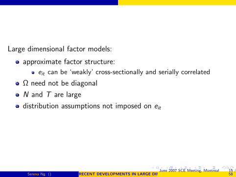
Large dimensional factor models:
approximate factor structure:
eit can be ‘weakly’ cross-sectionally and serially correlated
Ω need not be diagonal
N and T are large
distribution assumptions not imposed on eit
Serena Ng () RECENT DEVELOPMENTS IN LARGE DIMENSIONAL FACTOR ANALYSISJune 2007 SCE Meeting, Montreal 15 /
58
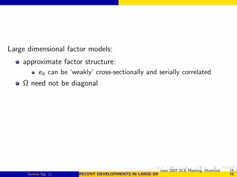
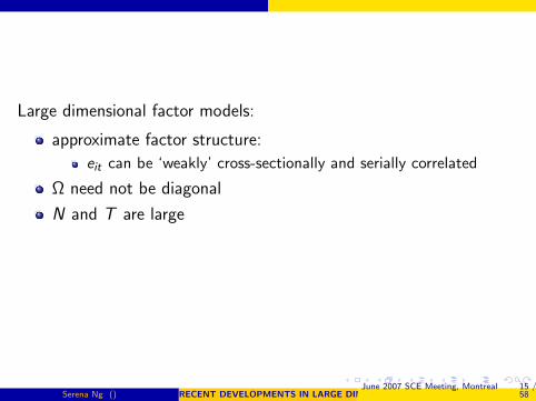
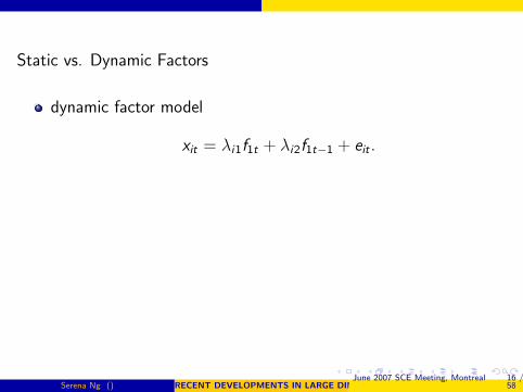
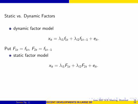
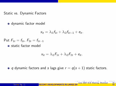
Static vs. Dynamic Factors
dynamic factor model
xit = λi1f1t + λi2f1t−1 + eit .
Put F1t = f1t , F2t = f1t−1
static factor model
xit = λi1F1t + λi2F2t + eit .
q dynamic factors and s lags give r = q(s + 1) static factors.
Serena Ng () RECENT DEVELOPMENTS IN LARGE DIMENSIONAL FACTOR ANALYSISJune 2007 SCE Meeting, Montreal 16 /
58
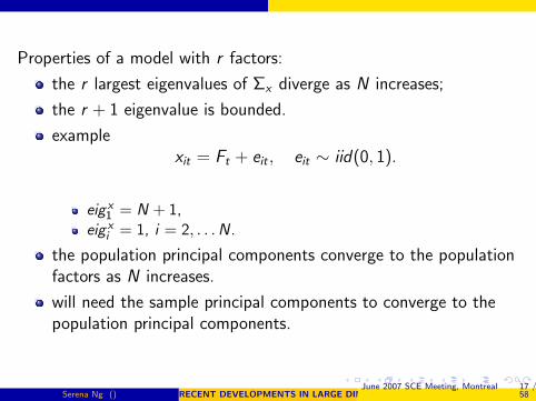
Properties of a model with r factors:
the r largest eigenvalues of Σx diverge as N increases;
the r + 1 eigenvalue is bounded.
examplexit = Ft + eit , eit ∼ iid(0, 1).
eig x1 = N + 1,
eig xi = 1, i = 2, . . . N.
the population principal components converge to the populationfactors as N increases.
will need the sample principal components to converge to thepopulation principal components.
Serena Ng () RECENT DEVELOPMENTS IN LARGE DIMENSIONAL FACTOR ANALYSISJune 2007 SCE Meeting, Montreal 17 /
58
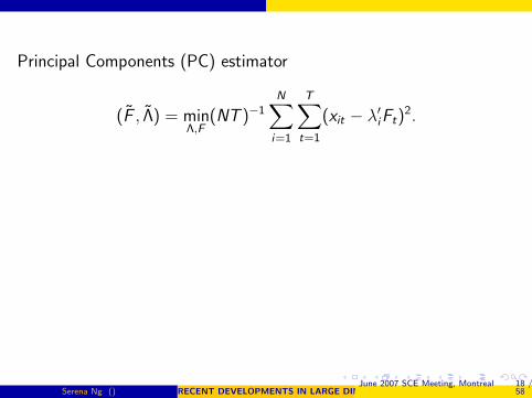
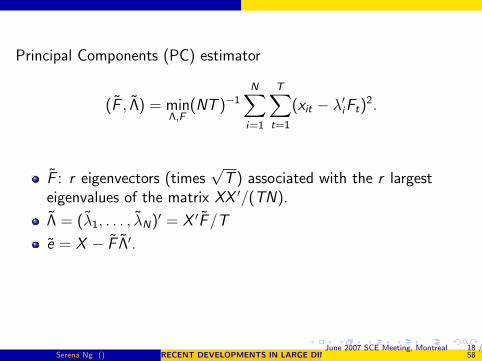
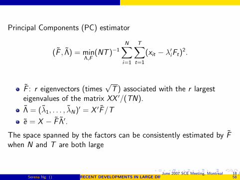
Principal Components (PC) estimator
(F , Λ) = minΛ,F
(NT )−1N∑
i=1
T∑t=1
(xit − λ′iFt)2.
F : r eigenvectors (times√
T ) associated with the r largesteigenvalues of the matrix XX ′/(TN).
Λ = (λ1, . . . , λN)′ = X ′F/T
e = X − F Λ′.
The space spanned by the factors can be consistently estimated by Fwhen N and T are both large
Serena Ng () RECENT DEVELOPMENTS IN LARGE DIMENSIONAL FACTOR ANALYSISJune 2007 SCE Meeting, Montreal 18 /
58
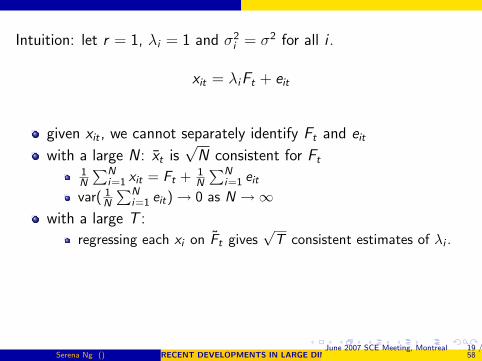
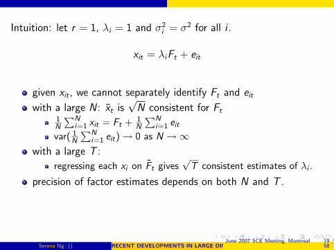
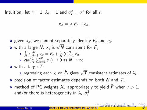
Intuition: let r = 1, λi = 1 and σ2i = σ2 for all i .
xit = λiFt + eit
given xit , we cannot separately identify Ft and eit
with a large N : xt is√
N consistent for Ft1N
∑Ni=1 xit = Ft + 1
N
∑Ni=1 eit
var( 1N
∑Ni=1 eit) → 0 as N →∞
with a large T :
regressing each xi on Ft gives√
T consistent estimates of λi .
precision of factor estimates depends on both N and T .
method of PC weights Xit appropriately to yield F when r > 1,and/or there is heterogeneity in λi , σ
2i .
Serena Ng () RECENT DEVELOPMENTS IN LARGE DIMENSIONAL FACTOR ANALYSISJune 2007 SCE Meeting, Montreal 19 /
58
Intuition: let r = 1, λi = 1 and σ2i = σ2 for all i .
xit = λiFt + eit
given xit , we cannot separately identify Ft and eit
with a large N : xt is√
N consistent for Ft
1N
∑Ni=1 xit = Ft + 1
N
∑Ni=1 eit
var( 1N
∑Ni=1 eit) → 0 as N →∞
with a large T :
regressing each xi on Ft gives√
T consistent estimates of λi .
precision of factor estimates depends on both N and T .
method of PC weights Xit appropriately to yield F when r > 1,and/or there is heterogeneity in λi , σ
2i .
Serena Ng () RECENT DEVELOPMENTS IN LARGE DIMENSIONAL FACTOR ANALYSISJune 2007 SCE Meeting, Montreal 19 /
58
Intuition: let r = 1, λi = 1 and σ2i = σ2 for all i .
xit = λiFt + eit
given xit , we cannot separately identify Ft and eit
with a large N : xt is√
N consistent for Ft1N
∑Ni=1 xit = Ft + 1
N
∑Ni=1 eit
var( 1N
∑Ni=1 eit) → 0 as N →∞
with a large T :
regressing each xi on Ft gives√
T consistent estimates of λi .
precision of factor estimates depends on both N and T .
method of PC weights Xit appropriately to yield F when r > 1,and/or there is heterogeneity in λi , σ
2i .
Serena Ng () RECENT DEVELOPMENTS IN LARGE DIMENSIONAL FACTOR ANALYSISJune 2007 SCE Meeting, Montreal 19 /
58
Intuition: let r = 1, λi = 1 and σ2i = σ2 for all i .
xit = λiFt + eit
given xit , we cannot separately identify Ft and eit
with a large N : xt is√
N consistent for Ft1N
∑Ni=1 xit = Ft + 1
N
∑Ni=1 eit
var( 1N
∑Ni=1 eit) → 0 as N →∞
with a large T :
regressing each xi on Ft gives√
T consistent estimates of λi .
precision of factor estimates depends on both N and T .
method of PC weights Xit appropriately to yield F when r > 1,and/or there is heterogeneity in λi , σ
2i .
Serena Ng () RECENT DEVELOPMENTS IN LARGE DIMENSIONAL FACTOR ANALYSISJune 2007 SCE Meeting, Montreal 19 /
58

Assumptions
F(0) – moments
LFE – independence
L – identification
E – weak correlation
IE – homoskedsaticity
Serena Ng () RECENT DEVELOPMENTS IN LARGE DIMENSIONAL FACTOR ANALYSISJune 2007 SCE Meeting, Montreal 20 /
58
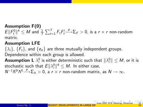
Assumption F(0)E‖F 0
t ‖4 ≤ M and 1T
∑Tt=1 FtF
′t
p−→ΣF > 0, is a r × r non-randommatrix.Assumption LFEλi, Ft, and eit are three mutually independent groups.Dependence within each group is allowed.Assumption L λ0
i is either deterministic such that ‖λ0i ‖ ≤ M , or it is
stochastic such that E‖λ0i ‖4 ≤ M . In either case,
N−1Λ0′Λ0 p−→ΣΛ > 0, a r × r non-random matrix, as N →∞.
Serena Ng () RECENT DEVELOPMENTS IN LARGE DIMENSIONAL FACTOR ANALYSISJune 2007 SCE Meeting, Montreal 21 /
58
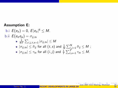
Assumption E:
b.i E (eit) = 0, E |eit |8 ≤ M .
b.ii E (eitejs) = σij ,ts1
NT
∑i ,j ,t,s=1 |σij ,ts | ≤ M
|σij ,ts | ≤ σij for all (t, s) and 1N
∑Ni ,j=1 σij ≤ M ;
|σij ,ts | ≤ τts for all (i , j) and 1T
∑Tt,s=1 τts ≤ M.
Serena Ng () RECENT DEVELOPMENTS IN LARGE DIMENSIONAL FACTOR ANALYSISJune 2007 SCE Meeting, Montreal 22 /
58
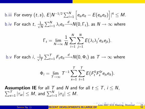
b.iii For every (t, s), E |N−1/2∑N
i=1
[eiseit − E (eiseit)
]|4 ≤ M .
b.iv For each t, 1√N
∑Ni=1 λieit
d−→N(0, Γt), as N →∞ where
Γt = limN→∞
1
N
N∑i=1
N∑j=1
E (λiλj′eitejt).
b.v For each i , 1√T
∑Tt=1 Fteit
d−→N(0,Φi) as T →∞ where
Φi = limT→∞
T−1T∑
s=1
T∑t=1
E (F 0t F 0′
s eiseit).
Assumption IE for all T and N and for all t ≤ T , i ≤ N ,∑Ts=1 |τst | ≤ M , and
∑Ni=1 |σij | ≤ M .
Serena Ng () RECENT DEVELOPMENTS IN LARGE DIMENSIONAL FACTOR ANALYSISJune 2007 SCE Meeting, Montreal 23 /
58
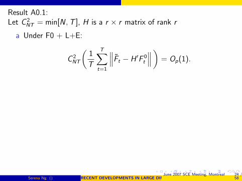
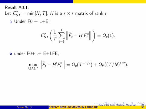
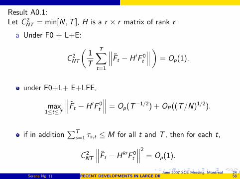
Result A0.1:Let C 2
NT = min[N ,T ], H is a r × r matrix of rank r
a Under F0 + L+E:
C 2NT
(1
T
T∑t=1
∥∥∥Ft − H ′F 0t
∥∥∥)= Op(1).
under F0+L+ E+LFE,
max1≤t≤T
∥∥∥Ft − H ′F 0t
∥∥∥ = Op(T−1/2) + OP((T/N)1/2).
if in addition∑T
s=1 τs,t ≤ M for all t and T , then for each t,
C 2NT
∥∥∥Ft − Hk′F 0t
∥∥∥2
= Op(1).
Serena Ng () RECENT DEVELOPMENTS IN LARGE DIMENSIONAL FACTOR ANALYSISJune 2007 SCE Meeting, Montreal 24 /
58
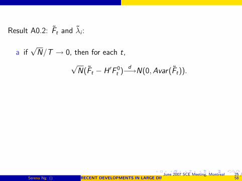
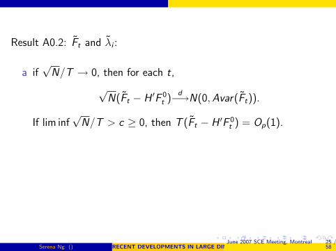
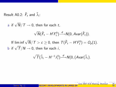
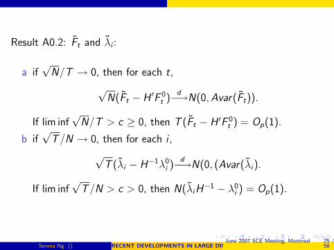
Result A0.2: Ft and λi :
a if√
N/T → 0, then for each t,
√N(Ft − H ′F 0
t )d−→N(0,Avar(Ft)).
If lim inf√
N/T > c ≥ 0, then T (Ft − H ′F 0t ) = Op(1).
b if√
T/N → 0, then for each i ,
√T (λi − H−1λ0
i )d−→N(0, (Avar(λi).
If lim inf√
T/N > c > 0, then N(λiH−1 − λ0
i ) = Op(1).
Serena Ng () RECENT DEVELOPMENTS IN LARGE DIMENSIONAL FACTOR ANALYSISJune 2007 SCE Meeting, Montreal 25 /
58
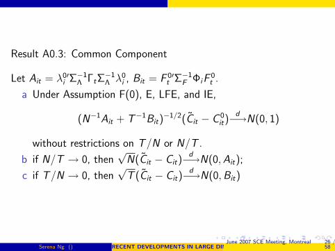
Result A0.3: Common Component
Let Ait = λ0′i Σ−1
Λ ΓtΣ−1Λ λ0
i , Bit = F 0′t Σ−1
F ΦiF0t .
a Under Assumption F(0), E, LFE, and IE,
(N−1Ait + T−1Bit)−1/2(Cit − C 0
it)d−→N(0, 1)
without restrictions on T/N or N/T .
b if N/T → 0, then√
N(Cit − Cit)d−→N(0,Ait);
c if T/N → 0, then√
T (Cit − Cit)d−→N(0,Bit)
Serena Ng () RECENT DEVELOPMENTS IN LARGE DIMENSIONAL FACTOR ANALYSISJune 2007 SCE Meeting, Montreal 26 /
58
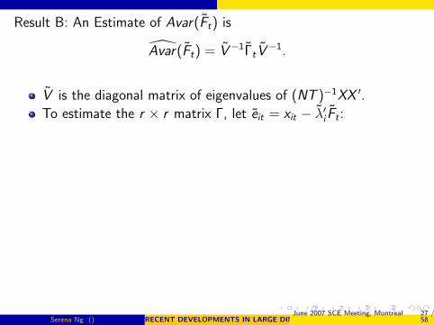
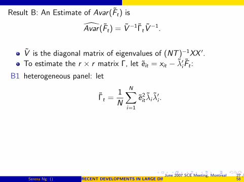
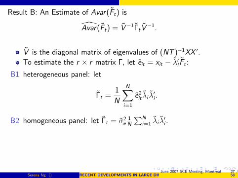
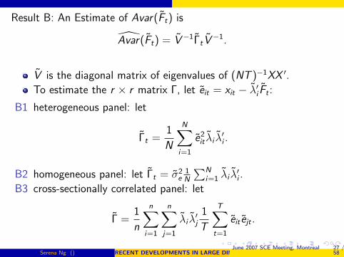
Result B: An Estimate of Avar(Ft) is
Avar(Ft) = V−1ΓtV−1.
V is the diagonal matrix of eigenvalues of (NT )−1XX ′.
To estimate the r × r matrix Γ, let eit = xit − λ′i Ft :
B1 heterogeneous panel: let
Γt =1
N
N∑i=1
e2it λi λ
′i .
B2 homogeneous panel: let Γt = σ2e
1N
∑Ni=1 λi λ
′i .
B3 cross-sectionally correlated panel: let
Γ =1
n
n∑i=1
n∑j=1
λi λ′j
1
T
T∑t=1
eit ejt .
Serena Ng () RECENT DEVELOPMENTS IN LARGE DIMENSIONAL FACTOR ANALYSISJune 2007 SCE Meeting, Montreal 27 /
58
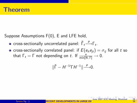
Theorem
Suppose Assumptions F(0), E and LFE hold,
cross-sectionally uncorrelated panel: Γtp−→Γt .
cross-sectionally correlated panel: if E (eitejt) = σij for all t sothat Γt = Γ not depending on t. If n
min[N,T ]→ 0.
‖Γ− H−1′ΓH−1‖ p−→0.
Serena Ng () RECENT DEVELOPMENTS IN LARGE DIMENSIONAL FACTOR ANALYSISJune 2007 SCE Meeting, Montreal 28 /
58
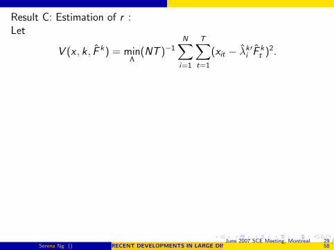
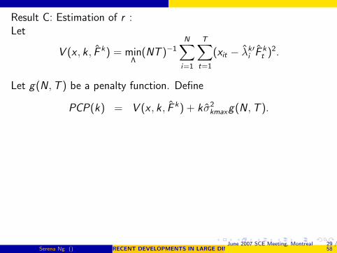
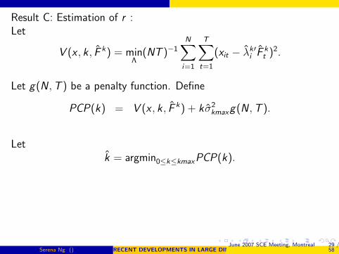
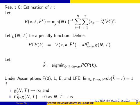
Result C: Estimation of r :Let
V (x , k , F k) = minΛ
(NT )−1N∑
i=1
T∑t=1
(xit − λk′i F k
t )2.
Let g(N ,T ) be a penalty function. Define
PCP(k) = V (x , k , F k) + k σ2kmaxg(N ,T ).
Letk = argmin0≤k≤kmaxPCP(k).
Under Assumptions F(0), L, E, and LFE, limN,T→∞ prob(k = r) = 1if
i g(N ,T ) →∞ and
ii C 2NTg(N ,T ) → 0 as N ,T →∞.
Serena Ng () RECENT DEVELOPMENTS IN LARGE DIMENSIONAL FACTOR ANALYSISJune 2007 SCE Meeting, Montreal 29 /
58
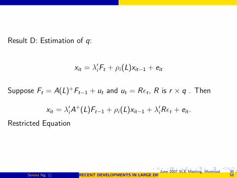
Result D: Estimation of q:
xit = λ′iFt + ρi(L)xit−1 + eit
Suppose Ft = A(L)+Ft−1 + ut and ut = Rεt , R is r × q . Then
xit = λ′iA+(L)Ft−1 + ρi(L)xit−1 + λ′iRεt + eit .
Restricted Equation
Serena Ng () RECENT DEVELOPMENTS IN LARGE DIMENSIONAL FACTOR ANALYSISJune 2007 SCE Meeting, Montreal 30 /
58
Result D: Estimation of q:
xit = λ′iFt + ρi(L)xit−1 + eit
Suppose Ft = A(L)+Ft−1 + ut and ut = Rεt , R is r × q . Then
xit = λ′iA+(L)Ft−1 + ρi(L)xit−1 + λ′iRεt + eit .
Restricted Equation
Serena Ng () RECENT DEVELOPMENTS IN LARGE DIMENSIONAL FACTOR ANALYSISJune 2007 SCE Meeting, Montreal 30 /
58

Let wit be the residuals from the restricted regressionLet
q = argminkPCP(k),
wherePCP(k) = V (w , k , F k) + k σ2
kmaxg(N ,T ).
Thenprob(q = q)
p−→1.
Serena Ng () RECENT DEVELOPMENTS IN LARGE DIMENSIONAL FACTOR ANALYSISJune 2007 SCE Meeting, Montreal 31 /
58
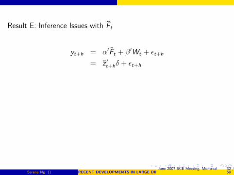
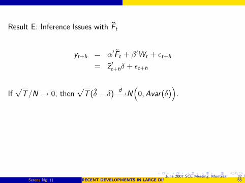
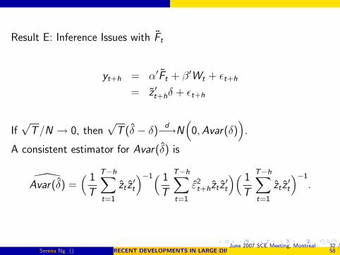
Result E: Inference Issues with Ft
yt+h = α′Ft + β′Wt + εt+h
= z ′t+hδ + εt+h
If√
T/N → 0, then√
T (δ − δ)d−→N
(0,Avar(δ)
).
A consistent estimator for Avar(δ) is
Avar(δ) =( 1
T
T−h∑t=1
zt z′t
)−1( 1
T
T−h∑t=1
ε2t+hzt z
′t
)( 1
T
T−h∑t=1
zt z′t
)−1
.
Serena Ng () RECENT DEVELOPMENTS IN LARGE DIMENSIONAL FACTOR ANALYSISJune 2007 SCE Meeting, Montreal 32 /
58
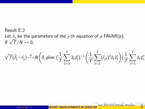
Result E.2Let δj be the parameters of the j-th equation of a FAVAR(p).
If√
T/N → 0,
√T (δj−δj)
d−→N
(0, plim (
1
T
T∑t=1
zt z′t)−1
(1
T
T∑t=1
(εjt)2zt z
′t
)(1
T
T∑t=1
zt z′t)−1
).
Serena Ng () RECENT DEVELOPMENTS IN LARGE DIMENSIONAL FACTOR ANALYSISJune 2007 SCE Meeting, Montreal 33 /
58
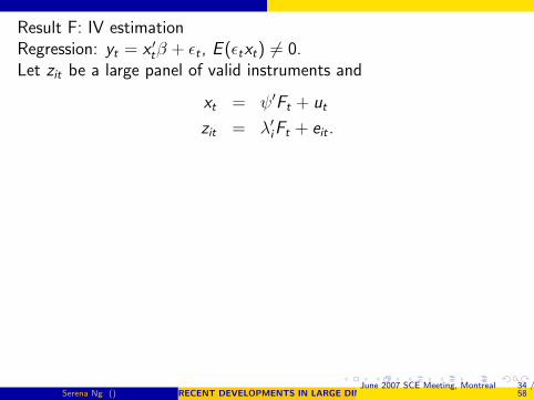
Result F: IV estimationRegression: yt = x ′tβ + εt , E (εtxt) 6= 0.Let zit be a large panel of valid instruments and
xt = ψ′Ft + ut
zit = λ′iFt + eit .
F1: Let gt = Ftεt . Then βFIV = β0 + op(1) ;
F2: If, in addition,√
TN→ 0 as N ,T →∞,
√T (βFIV − β0)
d−→N
(0,Avar(βFIV )
)where Avar(βFIV ) = plim (SF x(S)−1S ′
F x)−1.
F3: Let βIV be the estimator using z2 observed instruments. Then
Avar(βIV )− Avar(βFIV ) ≥ 0.
Serena Ng () RECENT DEVELOPMENTS IN LARGE DIMENSIONAL FACTOR ANALYSISJune 2007 SCE Meeting, Montreal 34 /
58
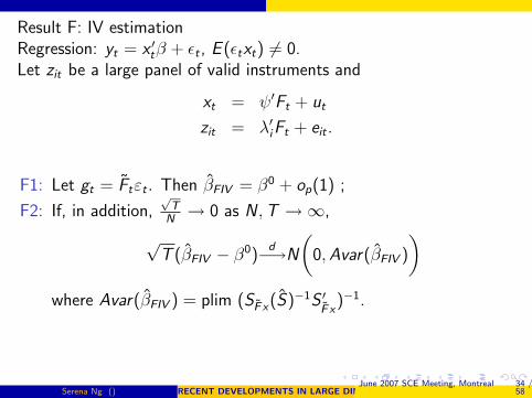
Result F: IV estimationRegression: yt = x ′tβ + εt , E (εtxt) 6= 0.Let zit be a large panel of valid instruments and
xt = ψ′Ft + ut
zit = λ′iFt + eit .
F1: Let gt = Ftεt . Then βFIV = β0 + op(1) ;
F2: If, in addition,√
TN→ 0 as N ,T →∞,
√T (βFIV − β0)
d−→N
(0,Avar(βFIV )
)where Avar(βFIV ) = plim (SF x(S)−1S ′
F x)−1.
F3: Let βIV be the estimator using z2 observed instruments. Then
Avar(βIV )− Avar(βFIV ) ≥ 0.
Serena Ng () RECENT DEVELOPMENTS IN LARGE DIMENSIONAL FACTOR ANALYSISJune 2007 SCE Meeting, Montreal 34 /
58
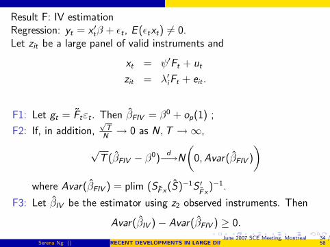
Result F: IV estimationRegression: yt = x ′tβ + εt , E (εtxt) 6= 0.Let zit be a large panel of valid instruments and
xt = ψ′Ft + ut
zit = λ′iFt + eit .
F1: Let gt = Ftεt . Then βFIV = β0 + op(1) ;
F2: If, in addition,√
TN→ 0 as N ,T →∞,
√T (βFIV − β0)
d−→N
(0,Avar(βFIV )
)where Avar(βFIV ) = plim (SF x(S)−1S ′
F x)−1.
F3: Let βIV be the estimator using z2 observed instruments. Then
Avar(βIV )− Avar(βFIV ) ≥ 0.
Serena Ng () RECENT DEVELOPMENTS IN LARGE DIMENSIONAL FACTOR ANALYSISJune 2007 SCE Meeting, Montreal 34 /
58

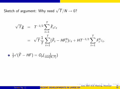
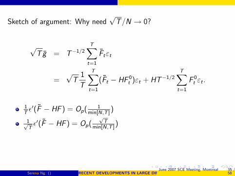
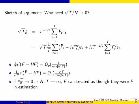
Sketch of argument: Why need√
T/N → 0?
√Tg = T−1/2
T∑t=1
Ftεt
=√
T1
T
T∑t=1
(Ft − HF 0t )εt + HT−1/2
T∑t=1
F 0t εt .
1Tε′(F − HF ) = Op(
1min[N,T ]
)
1√Tε′(F − HF ) = Op(
√T
min[N,T ])
if√
TN→ 0 as N ,T →∞, F can treated as though they were F
in estimation
Serena Ng () RECENT DEVELOPMENTS IN LARGE DIMENSIONAL FACTOR ANALYSISJune 2007 SCE Meeting, Montreal 35 /
58
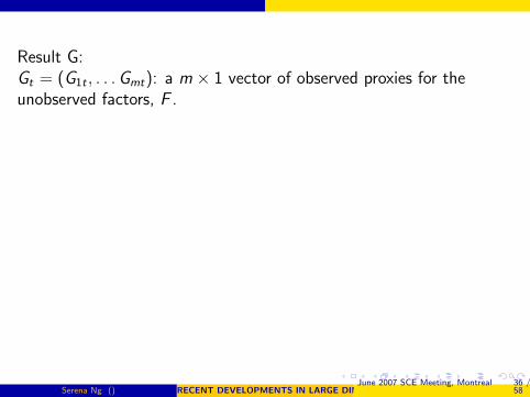
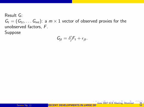
Result G:Gt = (G1t , . . .Gmt): a m × 1 vector of observed proxies for theunobserved factors, F .
SupposeGjt = δ′jFt + εjt .
Letεjt = Gjt − Gjt .
As N ,T →∞
εjt − εjtsjt
d−→N(0, 1)
s2jt = T−1F ′t(T
−1∑T
s=1 Fs F′s ε
2js)−1Ft + N−1Avar(Gjt),
Serena Ng () RECENT DEVELOPMENTS IN LARGE DIMENSIONAL FACTOR ANALYSISJune 2007 SCE Meeting, Montreal 36 /
58
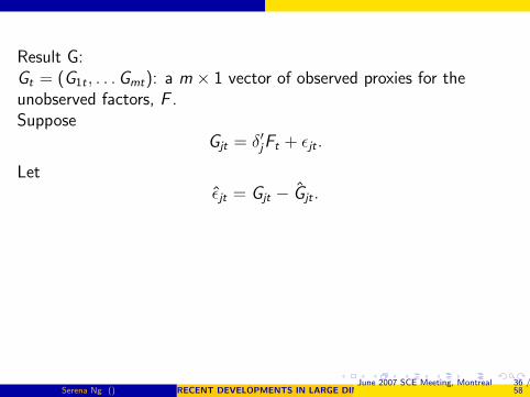
Result G:Gt = (G1t , . . .Gmt): a m × 1 vector of observed proxies for theunobserved factors, F .Suppose
Gjt = δ′jFt + εjt .
Letεjt = Gjt − Gjt .
As N ,T →∞
εjt − εjtsjt
d−→N(0, 1)
s2jt = T−1F ′t(T
−1∑T
s=1 Fs F′s ε
2js)−1Ft + N−1Avar(Gjt),
Serena Ng () RECENT DEVELOPMENTS IN LARGE DIMENSIONAL FACTOR ANALYSISJune 2007 SCE Meeting, Montreal 36 /
58
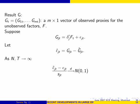
Result G:Gt = (G1t , . . .Gmt): a m × 1 vector of observed proxies for theunobserved factors, F .Suppose
Gjt = δ′jFt + εjt .
Letεjt = Gjt − Gjt .
As N ,T →∞
εjt − εjtsjt
d−→N(0, 1)
s2jt = T−1F ′t(T
−1∑T
s=1 Fs F′s ε
2js)−1Ft + N−1Avar(Gjt),
Serena Ng () RECENT DEVELOPMENTS IN LARGE DIMENSIONAL FACTOR ANALYSISJune 2007 SCE Meeting, Montreal 36 /
58
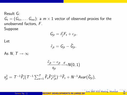
Result G:Gt = (G1t , . . .Gmt): a m × 1 vector of observed proxies for theunobserved factors, F .Suppose
Gjt = δ′jFt + εjt .
Letεjt = Gjt − Gjt .
As N ,T →∞
εjt − εjtsjt
d−→N(0, 1)
s2jt = T−1F ′t(T
−1∑T
s=1 Fs F′s ε
2js)−1Ft + N−1Avar(Gjt),
Serena Ng () RECENT DEVELOPMENTS IN LARGE DIMENSIONAL FACTOR ANALYSISJune 2007 SCE Meeting, Montreal 36 /
58
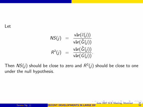
Let
NS(j) =var(ε(j))
var(G (j))
R2(j) =var(G (j))
var(G (j)).
Then NS(j) should be close to zero and R2(j) should be close to oneunder the null hypothesis.
Serena Ng () RECENT DEVELOPMENTS IN LARGE DIMENSIONAL FACTOR ANALYSISJune 2007 SCE Meeting, Montreal 37 /
58
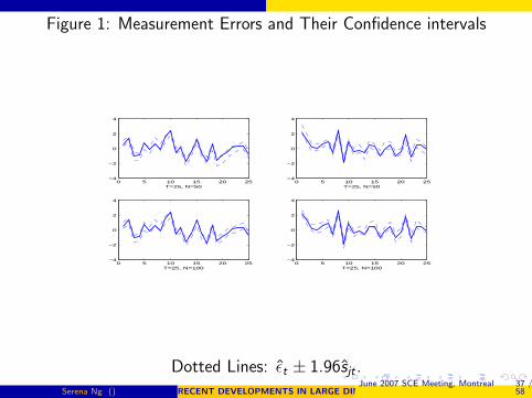
Figure 1: Measurement Errors and Their Confidence intervals
0 5 10 15 20 25−4
−2
0
2
4
T=25, N=500 5 10 15 20 25
−4
−2
0
2
4
T=25, N=50
0 5 10 15 20 25−4
−2
0
2
4
T=25, N=1000 5 10 15 20 25
−4
−2
0
2
4
T=25, N=100
Dotted Lines: εt ± 1.96sjt .
Serena Ng () RECENT DEVELOPMENTS IN LARGE DIMENSIONAL FACTOR ANALYSISJune 2007 SCE Meeting, Montreal 37 /
58
0 5 10 15 20 25−4
−2
0
2
4
T=25, N=500 5 10 15 20 25
−4
−2
0
2
4
T=25, N=50
0 5 10 15 20 25−4
−2
0
2
4
T=25, N=1000 5 10 15 20 25
−4
−2
0
2
4
T=25, N=100
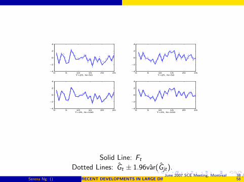
Solid Line: Ft
Dotted Lines: Gt ± 1.96var(Gjt).
Serena Ng () RECENT DEVELOPMENTS IN LARGE DIMENSIONAL FACTOR ANALYSISJune 2007 SCE Meeting, Montreal 38 /
58
Other applications:
consistent estimation of the factors without knowing if theidiosyncratic errors are I(0) or I(1) (spurious regressions)
individual unit root tests
panel unit root tests with cross-section dependence
panel cointegration analysis with cross-section dependence
Serena Ng () RECENT DEVELOPMENTS IN LARGE DIMENSIONAL FACTOR ANALYSISJune 2007 SCE Meeting, Montreal 38 /
58
Key to all the results:
the factor space can be consistently estimated by the method ofprincipal components when N and T are both large.
’ideal case’: iid data, min[T ,N] = 30 yields precise estimates
Serena Ng () RECENT DEVELOPMENTS IN LARGE DIMENSIONAL FACTOR ANALYSISJune 2007 SCE Meeting, Montreal 39 /
58
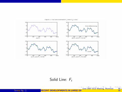
0 20 40 60 80 100-10
-5
0
5
10
(a) Ft
0 20 40 60 80 100-10
-5
0
5
10
(b) Ft and F t: N=20
↓First Differencing
0 20 40 60 80 100-10
-5
0
5
10
(c) Ft and F t: N=50 0 20 40 60 80 100
-10
-5
0
5
10
(d) Ft and F t: N=100
↑ Level
Figure 2: True and Estimated Ft when eit is I(0)
Solid Line: Ft
Serena Ng () RECENT DEVELOPMENTS IN LARGE DIMENSIONAL FACTOR ANALYSISJune 2007 SCE Meeting, Montreal 40 /
58
Practical issues
is the principal components estimator efficient?
are more data always better?
weak factor structure?
Serena Ng () RECENT DEVELOPMENTS IN LARGE DIMENSIONAL FACTOR ANALYSISJune 2007 SCE Meeting, Montreal 40 /
58

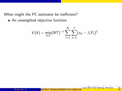
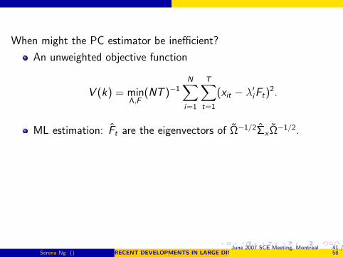
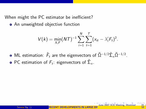
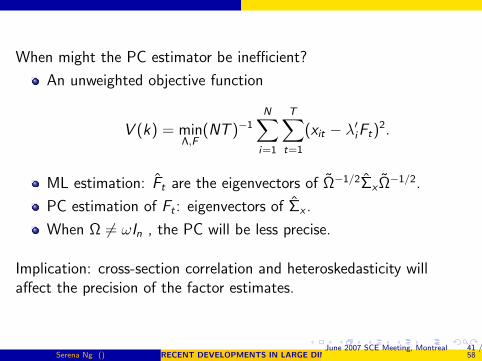
When might the PC estimator be inefficient?
An unweighted objective function
V (k) = minΛ,F
(NT )−1N∑
i=1
T∑t=1
(xit − λ′iFt)2.
ML estimation: Ft are the eigenvectors of Ω−1/2ΣxΩ−1/2.
PC estimation of Ft : eigenvectors of Σx .
When Ω 6= ωIn , the PC will be less precise.
Implication: cross-section correlation and heteroskedasticity willaffect the precision of the factor estimates.
Serena Ng () RECENT DEVELOPMENTS IN LARGE DIMENSIONAL FACTOR ANALYSISJune 2007 SCE Meeting, Montreal 41 /
58

How much data do we need?
If the additional data are informative about the factor structure,more data always yield more efficient estimates.
What if some of the data are ’noisy’, or have a weak factorstructure?
example (duplicated data) : N = 2N1. Then var(Ft) = Op(N−11 ).
Serena Ng () RECENT DEVELOPMENTS IN LARGE DIMENSIONAL FACTOR ANALYSISJune 2007 SCE Meeting, Montreal 42 /
58
the j-th eigenvalue of Σx measures the cumulative effect of the jfactor on the cross-section units.
strong factor asymptotics assumes that as N increases:
eig xr /eig x
r+1 →∞eig e
1 is bounded
Implication:
eig e1 /eig x
r ( noise to signal ratio ) should tend to zero
Serena Ng () RECENT DEVELOPMENTS IN LARGE DIMENSIONAL FACTOR ANALYSISJune 2007 SCE Meeting, Montreal 43 /
58

Why properties of eigenvalues are important?
if eig e1 is bounded, the population principal components
converge to the population factors as N increases
the sample principal components converge to the populationprincipal components as T increases (irrespective of N)
Serena Ng () RECENT DEVELOPMENTS IN LARGE DIMENSIONAL FACTOR ANALYSISJune 2007 SCE Meeting, Montreal 44 /
58
We assume 1N
∑i
∑j |E (eitejt)| < M .
fact: eig e1 ≤ maxi
∑j |E (eitejt)|
implication: eig e1 can be bounded and yet maxi
∑j |E (eitejt| can
increase with N .
we allow more cross-section correlation than if eig e1 is bounded.
Serena Ng () RECENT DEVELOPMENTS IN LARGE DIMENSIONAL FACTOR ANALYSISJune 2007 SCE Meeting, Montreal 45 /
58
Weak instrument asymptotics :
the least influential factor is comparable to the strongest idiosyncraticnoise.
when the r -th eigenvalue is too small,
F = FQ + F⊥
where Q is a random matrix with diagonal elements strictlysmaller than unity, and F⊥ is also random and orthogonal to F .
Two indicators of precision of the factor estimates.
eig xr+1/eig
xr
eig e1 /eig
xr
Serena Ng () RECENT DEVELOPMENTS IN LARGE DIMENSIONAL FACTOR ANALYSISJune 2007 SCE Meeting, Montreal 46 /
58
Weak instrument asymptotics :the least influential factor is comparable to the strongest idiosyncraticnoise.
when the r -th eigenvalue is too small,
F = FQ + F⊥
where Q is a random matrix with diagonal elements strictlysmaller than unity, and F⊥ is also random and orthogonal to F .
Two indicators of precision of the factor estimates.
eig xr+1/eig
xr
eig e1 /eig
xr
Serena Ng () RECENT DEVELOPMENTS IN LARGE DIMENSIONAL FACTOR ANALYSISJune 2007 SCE Meeting, Montreal 46 /
58
SimulationsFor i = 1, . . .N and t = 1, . . .T ,
xit = λ′i(L)ft + σieit
λi(L) = λi0 + λi1L + . . . λiLs .
σ2i is set so that R2
i ∼ U[R2L ,R
2U ],
R2U = .8.
λij ∼ N(0, 1)
Serena Ng () RECENT DEVELOPMENTS IN LARGE DIMENSIONAL FACTOR ANALYSISJune 2007 SCE Meeting, Montreal 47 /
58
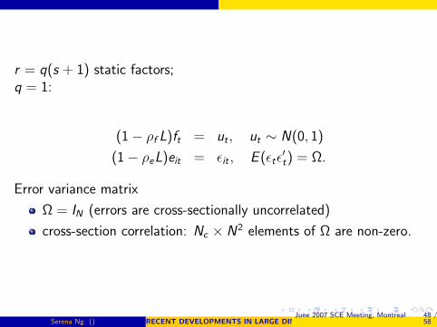
r = q(s + 1) static factors;q = 1:
(1− ρf L)ft = ut , ut ∼ N(0, 1)
(1− ρeL)eit = εit , E (εtε′t) = Ω.
Error variance matrix
Ω = IN (errors are cross-sectionally uncorrelated)
cross-section correlation: Nc × N2 elements of Ω are non-zero.
Serena Ng () RECENT DEVELOPMENTS IN LARGE DIMENSIONAL FACTOR ANALYSISJune 2007 SCE Meeting, Montreal 48 /
58
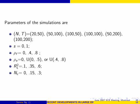
Parameters of the simulations are
(N ,T )=(20,50), (50,100), (100,50), (100,100), (50,200),(100,200);
s = 0, 1;
ρf = 0, .4, .8 ;
ρe=0, U(0, .5), or U(.4, .8)
R2L=.1, .35, .6;
Nc= 0, .15, .3;
Serena Ng () RECENT DEVELOPMENTS IN LARGE DIMENSIONAL FACTOR ANALYSISJune 2007 SCE Meeting, Montreal 49 /
58
For a given s and sample size: 81 configurations
total of 486 configurations
1000 replications each
keep track of eigenvalues
eig xr : average of the r -th largest eigenvalue of the matrx
Σxx = x ′x/(NT ) over 1000 replicationseig e
1 : the largest eigenvalue of Ω.EIGA,B(a, b): the ratio of the a-th largest eigenvalue of thecovariance matrix of A to the b-th largest eigenvalue of thecovariance matrix of B.
Let FIT= R2 from a regression of Ft on Ft and a constant.
Serena Ng () RECENT DEVELOPMENTS IN LARGE DIMENSIONAL FACTOR ANALYSISJune 2007 SCE Meeting, Montreal 50 /
58
Response surface analysis:Regress FIT on
C 2NT , CNT = min[
√N ,√
T ]
ratio of eigenvalues
non-linear terms
Serena Ng () RECENT DEVELOPMENTS IN LARGE DIMENSIONAL FACTOR ANALYSISJune 2007 SCE Meeting, Montreal 51 /
58
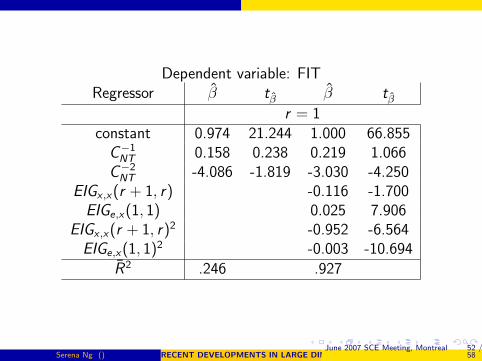
Dependent variable: FITRegressor β tβ β tβ
r = 1constant 0.974 21.244 1.000 66.855
C−1NT 0.158 0.238 0.219 1.066
C−2NT -4.086 -1.819 -3.030 -4.250
EIGx ,x(r + 1, r) -0.116 -1.700EIGe,x(1, 1) 0.025 7.906
EIGx ,x(r + 1, r)2 -0.952 -6.564EIGe,x(1, 1)2 -0.003 -10.694
R2 .246 .927
Serena Ng () RECENT DEVELOPMENTS IN LARGE DIMENSIONAL FACTOR ANALYSISJune 2007 SCE Meeting, Montreal 52 /
58
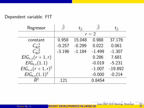
Dependent variable: FIT
Regressor β tβ β tβr = 2
constant 0.958 15.048 0.988 37.176C−1
NT -0.257 -0.299 0.022 0.061C−2
NT -3.196 -1.184 -1.499 -1.307EIGx ,x(r + 1, r) 0.286 7.681
EIGe,x(1, 1) -0.019 -5.231EIGx ,x(r + 1, r)2 -1.007 -19.892
EIGe,x(1, 1)2 -0.000 -0.214R2 .121 0.8454
Serena Ng () RECENT DEVELOPMENTS IN LARGE DIMENSIONAL FACTOR ANALYSISJune 2007 SCE Meeting, Montreal 53 /
58
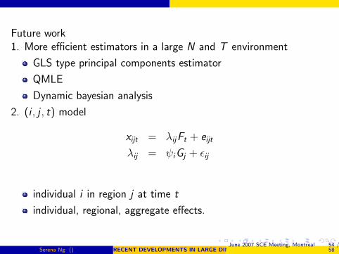
Future work1. More efficient estimators in a large N and T environment
GLS type principal components estimator
QMLE
Dynamic bayesian analysis
2. (i , j , t) model
xijt = λijFt + eijt
λij = ψiGj + εij
individual i in region j at time t
individual, regional, aggregate effects.
Serena Ng () RECENT DEVELOPMENTS IN LARGE DIMENSIONAL FACTOR ANALYSISJune 2007 SCE Meeting, Montreal 54 /
58
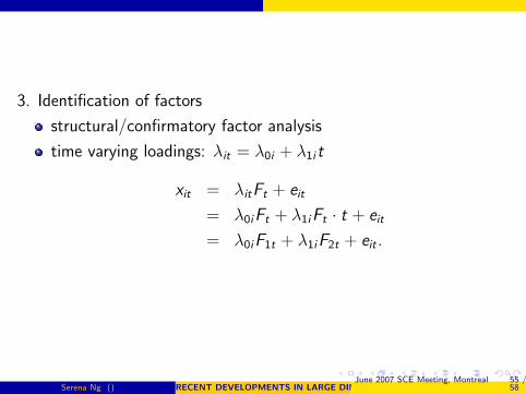
3. Identification of factors
structural/confirmatory factor analysis
time varying loadings: λit = λ0i + λ1i t
xit = λitFt + eit
= λ0iFt + λ1iFt · t + eit
= λ0iF1t + λ1iF2t + eit .
Serena Ng () RECENT DEVELOPMENTS IN LARGE DIMENSIONAL FACTOR ANALYSISJune 2007 SCE Meeting, Montreal 55 /
58
4. DSGE Models
small number of common shocks
stochastic singularitymeasurement error ⇒ factor structure
identification and estimation
Bayesian analysis in a large N and T setting
Serena Ng () RECENT DEVELOPMENTS IN LARGE DIMENSIONAL FACTOR ANALYSISJune 2007 SCE Meeting, Montreal 56 /
58
4. DSGE Models
small number of common shocks
stochastic singularitymeasurement error ⇒ factor structure
identification and estimation
Bayesian analysis in a large N and T setting
Serena Ng () RECENT DEVELOPMENTS IN LARGE DIMENSIONAL FACTOR ANALYSISJune 2007 SCE Meeting, Montreal 56 /
58
Conclusion:
the factor model is a useful way of achieving dimension reduction
factor estimates have good properties when N ,T are large
generated new theory and new applications
Serena Ng () RECENT DEVELOPMENTS IN LARGE DIMENSIONAL FACTOR ANALYSISJune 2007 SCE Meeting, Montreal 57 /
58

Thank You!
Serena Ng () RECENT DEVELOPMENTS IN LARGE DIMENSIONAL FACTOR ANALYSISJune 2007 SCE Meeting, Montreal 58 /
58