ÉCOLE DE TECHNOLOGIE SUPÉRIEURE UNIVERSITÉ DU QUÉBEC

THESIS PRESENTED TO ÉCOLE DE TECHNOLOGIE SUPÉRIEURE

IN PARTIAL FULFILLMENT OF THE REQUIREMENTS FOR A MASTER’S DEGREE IN ENGINEERING

M.Eng.

BY Bogdan Dumitru DANCILA

ALTITUDE OPTIMIZATION ALGORITHM FOR CRUISE, CONSTANT SPEED AND LEVEL FLIGHT SEGMENTS

MONTREAL, DECEMBER 15, 2011

©Copyright 2011 reserved by Bogdan Dumitru Dancila

II

©Copyright reserved

It is forbidden to reproduce, save or share the content of this document either in whole or in parts. The reader

who wishes to print or save this document on any media must first get the permission of the author.

BOARD OF EXAMINERS

THIS THESIS HAS BEEN EVALUATED

BY THE FOLLOWING BOARD OF EXAMINERS: Dr. Ruxandra Botez, Thesis Advisor Automated Manufacturing Engineering at École de technologie supérieure Dr. Guy Gauthier, President of the board of Examiners Automated Manufacturing Engineering at École de technologie supérieure Dr. Adrian Hiliuta, External Examiner CMC ELECTRONICS - ESTERLINE

THIS THESIS WAS PRESENTED AND DEFENDED

BEFORE A BOARD OF EXAMINERS AND PUBLIC

ON DECEMBER 12, 2011

AT ÉCOLE DE TECHNOLOGIE SUPÉRIEURE

FOREWORD

One of the main research and development objectives in the aeronautical industry consists in

the development of innovative equipment and algorithms that contribute to improving the

standards of economic efficiency and environmental protection. The Green Aviation

Research and Development Network (GARDN), a Business-Led Network of Centers of

Excellence (B-LNCE), regroups leading Canadian Aerospace Industry and Academic

Research Centers. GARDN actively promotes and supports projects and collaborative

research that address the environmental protection using green aircraft design.

Under GARDN auspices, the Research Laboratory in Active Controls, Avionics and

Aeroservoelasticity (LARCASE), at Ecole de Technologie Superieure (ETS), and CMC

Electronics-Esterline, are collaborating on a research project investigating new or improved

cruise and descent trajectory optimization algorithms for the CMC Electronics-Esterline’s

Flight Management System.

In this thesis, an algorithm is proposed that determines the optimal altitude that minimizes

the total costs for flying a constant speed, level flight, cruise segment. This algorithm is the

subject of the present thesis.

AKNOWLEDGEMENTS

Firstly, I would like to thank my supervisor, Professor Ruxandra Botez, for the opportunity to

perform my research at the Research Laboratory in Active Controls, Avionics and

Aeroservoelasticity (LARCASE), and for the opportunity to learn and work on interesting

aviation research projects. I would also like to express my deepest appreciation for her

mentorship as well as for academic and financial support throughout the Master’s program.

I would also like to thank to Mr. Dominique Labour from CMC Electronics – Esterline for

the excellent collaboration and for sharing his knowledge of practical aspects related to FMS

algorithm implementation. Many thanks are due to Mr Dominique Labour, Mr Rex Hygate,

Mr Daniel Guertin and Mr Claude Provencal for offering me the additional CMC Electronics

– Esterline scholarship. This scholarship gave me more encouragement to pursue and finalize

my Master thesis on the Green Aviation Research and Development Network (GARDN)

project, thus providing many learning opportunities and a great professional experience.

Also, I would like to thank my LARCASE colleagues, Ms. N. Dumondel and Messrs. J.

Dupont, R. Glumineau, J.Hemmerle, T. Klotz, B. Langlet, F. Millet, T. Salamah, S.

Souleymane, and L. Tevoedjre, for their collaboration and important contribution to

producing the FMS data needed for the algorithm validation.

A special thank to my family for their constant support throughout the duration of the

Master’s program.

ALTITUDE OPTIMIZATION ALGORITHM FOR CRUISE, CONSTANT SPEED AND LEVEL FLIGHT SEGMENTS

Bogdan Dumitru DANCILA

RÉSUMÉ

Dans ce mémoire le développement d’un algorithme est présenté. Dans cet algorithme, nous déterminons l’altitude optimale pour un vol de croisière, à une vitesse et altitude constantes, sur un segment donné de la trajectoire de vol. Le critère d’optimisation correspond à la minimisation des couts totaux, et, si possible, de la consommation de combustible, pour parcourir le segment de croisière spécifié. Le but principal est de prouver le concept d’un algorithme, pour une fonctionnalité du FMS, informant les pilotes sur l’altitude de vol optimale pour le segment de croisière considéré. L’algorithme a été développé en MATLAB, en utilisant une nouvelle méthode de calcul de la consommation de combustible pour les vols de croisière, à une vitesse et altitude constantes, en utilisant les données de performance de l’avion. Trois modèles d’avion ont été considérées, un pour lequel le modèle du vol de croisière prend en compte la position du centre de gravité, et deux modèles qui ne le font pas. L’algorithme a été développé pour des conditions normales de vol, et il ne prend pas en compte les couts correspondent aux changements d’altitude, au début et à la fin du segment, requises pour atteindre l’altitude optimale et revenir à l’altitude de croisière initiale. Les performances de l’algorithme ont été évaluées sur trois modèles d’avion – Airbus A310, Sukhoi RRJ et Lockheed L1011. Les données de validation ont été générées à partir des informations produites sur une plate-forme FMS de CMC Electronics – Esterline, qui utilise les mêmes modèles d’avion, et les mêmes données de performance, pour les mêmes conditions de vol Mots-clés : Flight Management System, altitude optimale de croisière, cout minimal, consommation de combustible

ALTITUDE OPTIMIZATION ALGORITHM FOR CRUISE, CONSTANT SPEED AND LEVEL FLIGHT SEGMENTS

Bogdan Dumitru DANCILA

ABSTRACT

In this thesis, the development of an algorithm is presented. The algorithm determines the optimal cruise altitude for flying an aircraft at a constant speed and altitude on a given segment of the flight route. The optimization criteria corresponds to the minimization of the total costs, and, if possible, fuel consumption, associated with flying the cruise segment. The main objective is the development of a new algorithm, for a functionality of the FMS platform, that will display for the pilots the advisory information on a segment’s cruise altitude yielding the minimal cost. The algorithm, developed in MATLAB, is using a new method for computing the fuel burn, for the level flight cruise segments, based on the aircraft’s performance data. Three aircraft models were considered, one whose cruise modeling uses the center of gravity position, and two that do not use the center of gravity position. The algorithm was developed for normal flight conditions, and does not consider the costs associated with the initial and final changes of altitude, necessary to reach the optimal altitude and, at the end of the segment, needed to return to the initial cruise altitude. Algorithm performances were evaluated on three aircraft models – Airbus A310, Sukhoi RRJ and Lockheed L1011. The validation data were generated based on the information produced on a CMC Electronics – Esterline FMS platform that used an identical aircraft model, and performance data, for identical flight conditions. Keywords: Flight Management System, optimal cruise altitude, minimal cost, fuel burn.

TABLE OF CONTENTS

Page

INTRODUCTION .....................................................................................................................1

CHAPTER 1 LITERATURE REVIEW ............................................................................3

CHAPTER 2 THEORETICAL ELEMENTS ....................................................................7 2.1 The fuel burn rate model for constant speed, level, cruise flight ...................................7 2.2 The total cost ..................................................................................................................8 2.3 The atmosphere ..............................................................................................................9

2.3.1 The standard atmosphere .......................................................................... 10 2.4 Mach number, IAS and TAS speeds. Crossover altitude .............................................12 2.5 The flight segment and the wind structure ...................................................................14 2.6 Aircraft ground speed, wind triangle and segment flight time ....................................15 2.7 Aircraft gross weight and center of gravity position ...................................................17 2.8 Maximal cruise altitude ................................................................................................19

CHAPTER 3 ALGORITHM DEVELOPMENT .............................................................21 3.1 The optimization strategy ............................................................................................21 3.2 Input variables ..............................................................................................................21

3.2.1 Optimization configuration parameters .................................................... 21 3.2.2 Aircraft design and performance data ....................................................... 22 3.2.3 Flight segment configuration .................................................................... 23 3.2.4 Aircraft configuration ............................................................................... 24

3.3 Output data ...................................................................................................................24 3.4 Algorithm processing steps ..........................................................................................25 3.5 Algorithm implementation ...........................................................................................25

3.5.1 TAS and crossover altitude module .......................................................... 26 3.5.2 The maximal cruise altitude and cruise altitude range module ................. 27 3.5.3 Ground speeds and segment flight times .................................................. 28 3.5.4 The fuel burn ............................................................................................. 28

3.5.4.1 The initialization module ........................................................... 29 3.5.4.2 The intermediary module ........................................................... 33 3.5.4.3 The fuel burn module ................................................................. 37

3.5.5 The total cost ............................................................................................. 38 3.5.6 The optimal altitude module ..................................................................... 38

CHAPTER 4 ALGORITHM VALIDATION ..................................................................39 4.1 The test results for Airbus A310 ..................................................................................43 4.2 The test results for Sukhoi RRJ ...................................................................................51 4.3 The test results for Lockheed L1011 ...........................................................................59

CONCLUSIONS......................................................................................................................61

XIV

RECOMMENDATIONS .........................................................................................................65

LIST OF BIBLIOGRAPHIC REFERENCES .........................................................................67

LIST OF TABLES

Page Table 4-1 Description of the A310 test configurations ..............................................43

Table 4-2 A310 optimal altitude test results function of the cost index value ..........44

Table 4-3 A310 performance results, function of the cost index value, as a difference between the algorithm computed values at the optimal altitudes computed using the algorithm and the PTT validation data ............................................................................................45

Table 4-4 A310 performance results, function of the cost index value, as the difference between the values computed using the algorithm and the PTT validation data, at the optimal altitude computed by the algorithm .........................................................................................46

Table 4-5 A310 Initialization module execution time statistics .................................48

Table 4-6 A310 Intermediary module execution time statistics.................................49

Table 4-7 A310 Optimal altitude module execution time statistics ...........................49

Table 4-8 Description of the RRJ test configurations ................................................51

Table 4-9 RRJ optimal altitude test results function of the cost index value ............52

Table 4-10 RRJ performance results, function of the cost index value, as a difference between the algorithm computed values at the optimal altitudes computed using the algorithm and the PTT validation data ............................................................................................53

Table 4-11 RRJ performance results, function of the cost index value, as the difference between the values computed using the algorithm and the PTT validation data, at the optimal altitude computed by the algorithm .........................................................................................54

Table 4-12 RRJ Initialization module execution time statistics ...................................56

Table 4-13 RRJ Intermediary module execution time statistics ...................................57

Table 4-14 RRJ Optimal altitude module execution time statistics .............................57

Table 4-15 L1011 tests description and fuel burn results ............................................60

LIST OF FIGURES

Page

Figure 2.1 “Wind triangle” diagram ............................................................................15

Figure 2.2 Aircraft weights and moments diagram .....................................................18

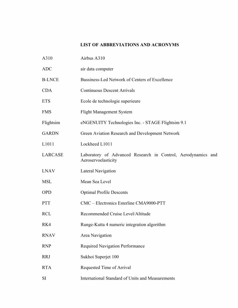
LIST OF ABBREVIATIONS AND ACRONYMS

A310 Airbus A310 ADC air data computer B-LNCE Bussiness-Led Network of Centers of Excellence CDA Continuous Descent Arrivals ETS Ecole de technologie superieure FMS Flight Management System Flightsim eNGENUITY Technologies Inc. - STAGE Flightsim 9.1 GARDN Green Aviation Research and Development Network L1011 Lockheed L1011 LARCASE Laboratory of Advanced Research in Control, Aerodynamics and

Aeroservoelasticity LNAV Lateral Navigation MSL Mean Sea Level OPD Optimal Profile Descents PTT CMC – Electronics Esterline CMA9000-PTT RCL Recommended Cruise Level/Altitude RK4 Runge-Kutta 4 numeric integration algorithm RNAV Area Navigation RNP Required Navigation Performance RRJ Sukhoi Superjet 100 RTA Requested Time of Arrival SI International Standard of Units and Measurements

XX

VNAV Vertical Navigation

LIST OF SYMBOLS AND MEASUREMENT UNITS alt altitude (ft) aLR air temperature variation coefficient (°R/ft) CAS calibrated airspeed (Kts) cg center of gravity position (%MAC) CGREFDIST aircraft center of gravity reference point’s position, as a distance from

the aircraft’s reference point (m) CG_AT_GW center of gravity position function of the total weight (%MAC) CG_SLOPE center of gravity position variation coefficient (%MAC) CI cost index (Kg/min) Ctot total cost ($) CTOT total cost (Kg) datum the longitudinal reference point of the aircraft (dimensionless) dcg center of gravity position variation (%MAC) deg degrees δ pressure ratio (dimensionless) dgw gross weight variation (Kg) $ US dollars fbr fuel burn rate (Kg/h) FC fuel cost ($) fcr fuel correction factor (dimensionless) ff fuel flow (Kg/h) fuel fuel weight (Kg)

XXII

Fuelprice fuel price ($/Kg) ft foot γ adiabatic constant of the ideal gas (dimensionless) GS ground speed (Kts) gw gross weight (Kg) h hour IAS indicated airspeed (Kts) ISA_Dev air temperature deviation from the value corresponding to the standard

atmosphere (°K) °K Kelvin Kg kilogram Kts Knots lb pound lbf Pound-force LEMAC the leading-edge, mean aerodynamic chord position with respect to the

datum (m) m meter Ma aircraft moment (Kg m) Mf fuel moment (Kg m) Mfgw fuel moment expressed as a function of the total weight (Kg m) min minute MIN_ALTITUDE minimal cruise altitude (ft) mmo maximum operational Mach index (dimensionless) Mt total moment (Kg m)

XXIII

MAC Mean Aerodynamic Chord (m) %MAC percentage of MAC (dimensionless) Mach Mach index (dimensionless)

NFC non fuel cost ($) Nm nautical mile OAT outside air temperature (°K) OPT_DISTANCE cruise segment length / optimization distance (Nm) p air pressure (lb/ft2) pSL standard atmosphere, mean sea level air pressure(lb/ft2) R ideal gas constant (ft lbf / slug °R) °R Rankine ρ air density (slug/ft3) ρSL standard atmosphere, mean sea level air density (slug/ft3) slug Slug – imperial weight unit σ density ratio (dimensionless) T air temperature (°K) TSL standard atmosphere, mean sea level air temperature (°K) Tflight cruise segment’ flight time (h) TAS true air speed (Kts) temp temperature (°K) vmo maximum operational IAS speed (Kts) WA wind angle (deg)

XXIV

WCA wind correction angle, or crabbing angle (deg) WV wind speed (Kts) zfgw zero fuel gross weight (Kg) zfwcg zero fuel weight center of gravity position (%MAC)

INTRODUCTION

The Flight Management System (FMS) is an important element of modern aviation. Its

capabilities have a direct, and major, impact in terms of flight safety, environmental and

economical performances. This thesis presents the development of an algorithm for a Flight

Management System. This algorithm will determine the optimal cruise altitude for an aircraft

flying on a given distance of its flight plan’s cruise segment, at constant speed and altitude.

The algorithm will yield the minimal total flight costs for the given flight distance.

A number of limitations were imposed in the development of the algorithm, which:

• Must be deterministic, meaning that at any time, an identical set of input parameters must

conduct to an “identical” algorithm response.

• Must be compatible with the real-time nature of the FMS application. The modules

requiring more time or processing resources must be executed as least as possible and

should not affect the application’s response time.

• Is compatible with the aircraft performance and capabilities description model, based on

linear interpolation tables, used by the FMS platform.

• Is applicable to aircraft cruise performance description models as given by CMC

Electronics that are dependent of the center of gravity position (cg), and with models that

are not.

The other limitations of the algorithm are:

• Only normal cruise operation conditions are considered. One engine operation or other

abnormal conditions are not considered.

• The altitude optimization is performed for a cruise segment, defined by its heading and

length.

• The cruise segment performances are evaluated at altitudes that are multiples of 1,000 ft.

These altitudes are situated between a minimum altitude, provided as an algorithm input

parameter, and aircraft’s maximum attainable altitude, function of its performances,

2

capabilities and its configuration (gross weight, center of gravity position, speed etc.) at

the start of the segment.

• No time constraints were considered (such as Requested Time of Arrival, RTA, and

arrival error cost function which factors the costs incurred for not observing the

waypoints’ arrival time constraints).

• At each altitude, the performances are evaluated for constant speeds.

• Aircraft speed is described by the speed schedule, defined by CMC Electronics as a

couple of Indicated Air Speed (IAS) and Mach number (Mach) values. Their use is

function of the crossover altitude, defined as the altitude at which the true air speed (TAS)

computed using the IAS equals the TAS computed using the Mach number. The IAS value

is used below crossover altitude, and the Mach value is used at or above crossover

altitude.

• Two wind scenarios, associated with the cruise segment, are considered: still air (no

wind), and constant wind. In the case of constant wind, the wind structure, describes the

wind speed and direction at up to four altitudes, and is constant along the segment length.

• If a set of two or more altitudes yield the minimal cost, the selected optimal altitude

corresponds to the altitude, in the set, also yielding the minimal quantity of burned fuel.

The first chapter reviews the current state of the art, related to the FMS and the cruise

optimization algorithms. Subsequently, the second chapter details the main theoretical

concepts used in the development of the algorithm. The third chapter presents the algorithm

implementation for each of the two considered aircraft performance models. In chapter four,

the results obtained with this algorithm are presented, and compared with the corresponding

results, computed using the flight time and fuel burn information, generated on a PC-based

FMS simulator. Finally, the conclusions and the recommendations for future work are

presented.

CHAPTER 1

LITERATURE REVIEW

The avionics industry has a continuous and special interest in augmenting the performances

and capabilities of the FMS. This is determined by two factors: first, the introduction of new

aviation standards and requirements; second, the ongoing increase in computing power and

the development of new hardware and algorithms. An analysis of Liden [1] provides a

comprehensive description of the development and evolution of the FMS, at Honeywell,

since its initial design, in 1982. In a more recent work, Herndon et al. [2] describe some of

the current key FMS concepts and directions of development, including Area Navigation

(RNAV), Required Navigation Performance (RNP), Optimal Profile Descents (OPDs), and

Continuous Descent Arrivals (CDA). A comparative analysis of the capabilities and

performances of several modern FMS equipment is also provided.

As presented by Liden [1], two important sets of FMS functions, for performance prediction

and for performance optimization, are used to compute flight trajectories that attain specific

objectives (such as lateral navigation – LNAV, vertical navigation – VNAV, and cost or fuel

burn optimization), while observing various constraints (such as speed, altitude, time or fuel

burn). Past and current economic, and climatic, developments accentuated the interest for the

development of new or improved FMS flight performance prediction and trajectory

optimization algorithms and functions. One important class of performance optimization

objectives refers to the determination of optimum cruise altitude profiles with the aim to

minimize the flying costs incurred in flying a part of, or the entire cruise segment of the flight

plan Liden [3]. The optimal cruise profile may consider time, as shown by Liden [4], or other

constraints, such as arrival error cost functions, see Liden [5]. The optimization process may

be approached from different perspectives, such as energy-state equations Liden [5] and

Shufan Wu et al. [6], or aircraft’s performance and capabilities model, based on linear

interpolation tables Liden [3].

4

The algorithm developed in the present thesis is based on the method that uses the aircraft’s

performance and capabilities model - described by Liden [3]. The computation of the optimal

cruise altitude, also called the recommended cruise altitude (RCL), for a segment of a

determined length, at constant speed, in level-flight conditions, was achieved by performing

a series of forward predictions. The method described by Liden [3] determined the maximal

altitude to use for the cruise segment, as a function of the current aircraft parameters (such as

gross weight), selected speed and atmospheric conditions. Then the set of altitudes

considered in the process of optimization were determined, by applying a set of restrictions

imposed by the aircraft’s performances and capabilities. For each altitude, the segment length

was decomposed in intervals of up to 50Nm, on which the ground speed, corresponding

flight times, and fuel burns were computed. The fuel burn was computed using the fuel flow

(ff) performance parameter, expressed in kg/h, as a function of the aircraft speed, gross

weight (gw), outside air temperature, and altitude. The fuel flow, considered constant on each

interval, and equal to the value computed at the beginning of the interval, was integrated to

produce the fuel burn. The cruise segment’s total fuel burn and flight time, at each altitude,

were computed as the sum of the fuel burns, and flight times respectively, of the

corresponding intervals. Subsequently, the total cost, at each altitude was computed as the

sum of the fuel cost, corresponding to the total fuel burn, and the non fuel cost. The non fuel

cost was found to be proportional to the cruise segment’s total flight time, by a factor called

the Cost Index (CI), expressed as the ratio between the price of one kilogram of fuel, and the

non fuel cost for one minute of flight. Finally, the total cost values, corresponding to the set

of altitudes, were compared and the altitude yielding the minimal total cost was selected as

the optimal altitude.

The algorithm developed in this thesis, however, presents two main differences related to the

constant speed, constant altitude, cruise, fuel flow modeling and fuel burn computation. It

computes the instantaneous fuel consumptions, expressed in kg/h, called the fuel burn rates

(fbr), as a product between the fuel flow (ff) and a new parameter, the fuel correction factor

(fcr). The fuel correction factor, expressed as a dimensionless value, allows a more flexible,

aircraft cruise fuel burn modeling than the Liden’s approach described in the previous

5

paragraph. Two fcr function models are considered, the first function considers the fcr as a

constant value, while the second function considers the fcr as a function of the aircraft center

of gravity position (cg), speed, gross weight, and altitude. The algorithm also considers the

continuous variation of the fbr along the cruise flight segment, and computes the fuel burn as

the integral value of the fbr along the entire cruise segment length (flight time). Therefore,

the value of the fuel burn, and the total cost, computed by the algorithm developed in this

thesis are more accurate than the value computed considering a constant fuel burn rate, as

described by Liden [3]. It also allows the computation of the fuel burn value for the entire

cruise segment, without the constraint of decomposing it in sub-segments, irrespective of its

length.

CHAPTER 2

THEORETICAL ELEMENTS

The main theoretical concepts and elements used in the development of the algorithm are

presented in this chapter. The cruise fuel burn model and the structure of the total flight cost

are described in sections 2.1 and 2.2. The standard atmosphere and the relationship between

the indicated air speed (IAS), Mach number (Mach), and the true air speed (TAS) are

presented in sections 2.3 and 2.4. The relationship between the aircraft’s TAS, the wind, and

the aircraft’s ground speed is then presented in section 2.5 and 2.6. The method used to

compute the position of the center of gravity of an aircraft is then described, in section 2.7,

and followed by the elements that determine the aircraft’s maximal cruise altitude, in section

2.8.

2.1 The fuel burn rate model for constant speed, level, cruise flight

The fuel burn rate (fbr) model, employed in the present thesis, is obtained from the model

that uses a fuel flow linear interpolation table, described by Liden [3], as a function of the

aircraft’s altitude, speed, outside air temperature and gross weight.

A new parameter, fuel correction factor (fcr), that multiplies the fuel flow (ff), allows a better

characterization of the cruise flight. We considered two descriptions of the fcr, one as a

constant value, and another as a linear interpolation table, as a function of the aircraft’s

speed, gross weight, center of gravity position, and altitude. Therefore, depending on the

chosen fuel correction factor model, the equation describing the fbr can have one of the

following expressions:

( ) ( ), , , , , , *fbr speed gw temp alt ff speed gw temp alt fcr= (2.1)

or

8

( ) ( ) ( ), , , , , , , * , , ,fbr speed gw temp alt cg ff speed gw temp alt fcr speed gw cg alt= (2.2)

The two equations describe the fbr value at one specific moment in time (t), for the

corresponding set of input parameters: speed, gw, temp, alt, cg. However, the input

parameters’ values may constantly change during the flight. Therefore, it is appropriate to

consider the ff, fcr, and fbr as a function of time. Consequently, the equation describing the

fbr can also be written as follows:

( ) ( ) ( )*fbr t ff t fcr t= (2.3)

2.2 The total cost

The cost model used in the present thesis, described by Liden [5] and Liden [3], computes the

total cost (Ctot) associated with a flight as a sum of two factors: fuel cost (FC), and non-fuel

operational cost (NFC).

totC FC NFC= + (2.4)

The fuel cost is the price, in dollars, of the quantity of fuel burned (FB) on the considered

flight. It is computed as the product between the price of a kilogram of fuel (Fuelprice) and the

integral sum of the fuel burn rate (fbr) over the entire segment distance.

The non-fuel operational cost factor represents the sum of all non-fuel costs incurred for

flying the considered trajectory. As described by Liden [3], its value, in dollars, is computed

as the product between the segment flight time (Tflight) and a cost index (CI). The cost index

is a parameter, whose value is established by the airline company, representing the non-fuel

operational cost, expressed in kilograms of fuel, for a minute of flight.

Usually, the duration of the flight is expressed in hours. Therefore, using equation (2.3) that

considers the fbr as a function of time, the total cost, expressed in dollars, is described by the

equation:

9

( )

0

* * 60* *flightT

tot price flightC Fuel fbr t dt CI T

= +

(2.5)

The total cost can be expressed independently of the price of fuel, by eliminating the Fuelprice

factor. Consequently, the equation describing the total cost, expressed in kilograms of fuel,

becomes:

( )

0

* 60* *flightT

TOT flightC fbr t dt CI T= + (2.6)

2.3 The atmosphere

Aerodynamic lift is one of the fundamental flight elements. It is produced by the relative

motion between an airfoil and its surrounding mass of air (atmosphere), measured as the

airspeed. Consequently, accurate measurement of the airspeed is essential for maintaining a

stable, controlled flight. Therefore, it is important to have a good understanding and

characterization of the atmosphere, and its parameters. The atmosphere parameters that

characterize the unit volume of air are the pressure (p), density (ρ) and temperature (T). The

pressure can correspond to the static pressure (ps), determined by the weight of the air

column situated above the measure point, the impact (or dynamic) pressure (qc)

corresponding to the kinetic energy of the moving mass of air, and the total pressure (pT), as

the sum of the static and dynamic pressures. These pressures can be expressed in SI (metric)

or English units.

The variation of the air pressure, density and temperature is described by the equation of the

ideal gas, as indicated by Aselin [7], Botez [8], and by other authors in the classical

references:

p RTρ= (2.7)

10

Where R, the gas constant, is equal to 287 J/kg °K or 1716 ft lbf / slug ºR

As atmospheric parameters change with time and location, it is also important to define

aircraft performances with respect to a set of known, stable, atmospheric parameters values,

called the standard atmosphere. It is thus possible to determine, and compare, aircraft

performances in different atmospheric conditions.

2.3.1 The standard atmosphere

The standard atmosphere defines the proprieties of the atmosphere at a reference altitude, the

mean sea level (MSL), where the air is dry, and behaves as an ideal gas. The reference values

of the atmosphere parameters are defined and presented in the literature, such as Asselin [7]

and Botez [8], for various sets of metric, and English, units.

For the range of altitudes corresponding to a normal flight, up to 21,000m = 21Km, the

atmosphere is composed of two layers: the troposphere, from 0 to 11Km = 36,089 ft, where

the temperature decreases linearly with the altitude, and the stratosphere, between 11Km =

36,089ft and 21Km = 70,000ft, where the temperature is constant. The air pressure and its

density decrease with the altitude. The law of variation, for each of the parameters, is

dependent on the atmosphere layer for which their values are computed, troposphere or

stratosphere. In troposphere, the variation of the parameters, as described by Asselin [7] and

Botez [8], is as follows: The temperature variation, with the altitude, is governed by the

following equation:

h SL LRT T a h= + (2.8)

(Asselin [7], page 312)

where aLR is the temperature variation coefficient, which is -0.0065°K/m or

-0.00356 ºR/ft. The pressure variation with the altitude is described by the equation:

11

( )LRg a R

hh SL

SL

Tp p

T

−

=

(2.9)

(Asselin, [7], page 312)

The density variation with the altitude is described by the equation:

( )1 LRg a R

hh SL

SL

T

Tρ ρ

− −

=

(2.10)

(Asselin, [7], page 313)

In stratosphere, as described by Botez [8], due to the fact that the temperature is constant, the

pressure and density laws of variation are defined by the equations:

0

strat

strat

g h

RTstratp p e

Δ−=

(2.11)

0

strat

strat

g h

RTstrateρ ρ

Δ−=

(2.12)

where Tstrat is the stratosphere temperature (216.66°K, -56.5ºC, or 390ºR), p0strat and ρ0strat are

the pressure and the density, at the initial stratosphere altitude of 11Km, and Δhstrat is the

altitude measured with respect to the initial stratosphere altitude.

It is often useful to compare aircraft performances, or atmosphere parameters, at different

altitudes, in the simplest way possible. The comparisons can be achieved by defining a set of

parameters: temperature ratio (θ), pressure ratio (δ), and density ratio (σ). As described by

12

Asselin [7] and Botez [8], their values are computed, for any given altitude h, by dividing the

value of the corresponding parameter at altitude h, by its, standard value at the MSL.

Another important parameter is the speed of sound (a), which is computed, as described by

Asselin [7], Botez [8] and by other authors in the classical references, using the equation:

a RTγ= (2.13)

where γ = 1.4 is the adiabatic constant of the ideal gas.

The atmospheric temperature, pressure, density, or their corresponding ratios, along with the

speed of sound variations with the altitude, are summarized in the literature, such as Asselin

[7] and Botez [8], as a standard atmosphere definition table.

In reality, the pressure, density and temperature values at the MSL are different than those

defined for the standard atmosphere. One parameter, the temperature, is used to compute

many aircraft performance data, including the fuel burn and the maximal altitude. The

temperature difference with respect to the MSL is defined with respect to the standard

atmosphere temperature. This parameter, called standard temperature deviation (ISA_Dev),

provides a proper way of characterizing aircraft performances as a function of atmosphere

variation.

2.4 Mach number, IAS and TAS speeds. Crossover altitude

On-board aircraft sensors, pitot-tubes and static pressure probes, measure the total pressure –

representing the sum of the static and the impact pressure, and the static atmospheric

pressure, respectively. This information is processed by the air data computer (ADC), to

produce three speed parameters: the indicated air speed (IAS), the Mach number (Mach), and

the true air speed (TAS).

13

For the standard atmosphere, and compressible flow regions, the TAS is computed based on

the dynamic and static pressures measured by the pitot-tube, using the equation:

( )1

021 1

1

p ppTAS

p

γγγ

γ ρ

− − = + − −

(2.14)

(Asselin, [7], page 323)

The IAS value actually represents the value of the calibrated airspeed (CAS), measured by the

airspeed indicator. This value is equal to the TAS only at the sea level, for the standard

atmosphere conditions. As described by Botez [8], the TAS for a given altitude is obtained

from the IAS, by compensating for the density and pressure variation with altitude. First, the

differential pressure, qc, corresponding to sea level, standard atmosphere conditions, is

computed from the IAS value using the equation:

( )1

20

11 1

2SL

c SLSL

q p p p IASp

γγργ

γ−

− = − = + −

(2.15)

which is obtained from the equation (2.14). Then, the pressure (p), and density (ρ), at the

considered altitude are expressed as a function of the standard atmosphere, sea level values,

and the pressure ratio (δ) and density ratio (σ) corresponding to that altitude. Finally, they are

replaced in equation (2.14), and the final form of the equation that computes the TAS is

obtained:

1

21 1

1SL c

SL SL

p qTAS

p

γγγ δ

γ ρ σ δ

− = + − −

(2.16)

14

The TAS value corresponding to a given Mach number is computed, as indicated by Asselin

[7] and Botez [8], using the equation:

( ) ( )*TAS h Mach a h= (2.17)

where a(h) represents the speed of sound at the altitude for which the TAS is computed.

For a speed schedule composed of a Mach number and an IAS speed, the crossover altitude

is the altitude at which the TAS value computed using the Mach number equals the TAS value

computed using the IAS speed. Below the crossover altitude, the aircraft operation and

parameters are referred to the IAS speed. At and above the crossover altitude, the aircraft

operation and parameters are referred to the Mach number.

2.5 The flight segment and the wind structure

The FMS performs the navigation and performance predictions, and guides the aircraft

according to the flight plan entered by the pilots as a series of waypoints and airways. The

waypoints are usually selected from the FMS’ navigation database. The waypoints can also

be entered manually using their geographic coordinates, or positions (distances, angles, or

both) relative to one or two waypoints or navigation aid systems. Once the waypoints

selected, the FMS computes the length and the heading of each of the segments determined

by two consecutive waypoints.

Each waypoint may have a number of parameters, and restrictions, that apply to the segment

starting at that waypoint. They may refer to altitude, speed schedule (IAS, Mach, or both),

wind structure, standard temperature deviation (ISA_Dev), Requested Arrival Times, etc.

If the segment speed schedule is configured as a pair of IAS and Mach values, the IAS value

is used below, while the Mach value is used at and above the crossover altitude. The wind

structure defines the wind layers, as the direction from which they blow, relative to the

North, and their speeds, in Knots. Modern FMS, as described by Liden [1], can associate to

15

each waypoint a structure characterizing the winds at up to four altitudes. At any altitude, the

wind is computed through interpolation, using the values shown in the wind structure table.

For the scope of the present thesis, we only consider the parameters that describe the segment

length, heading, speed schedule, wind structure, and ISA_Dev.

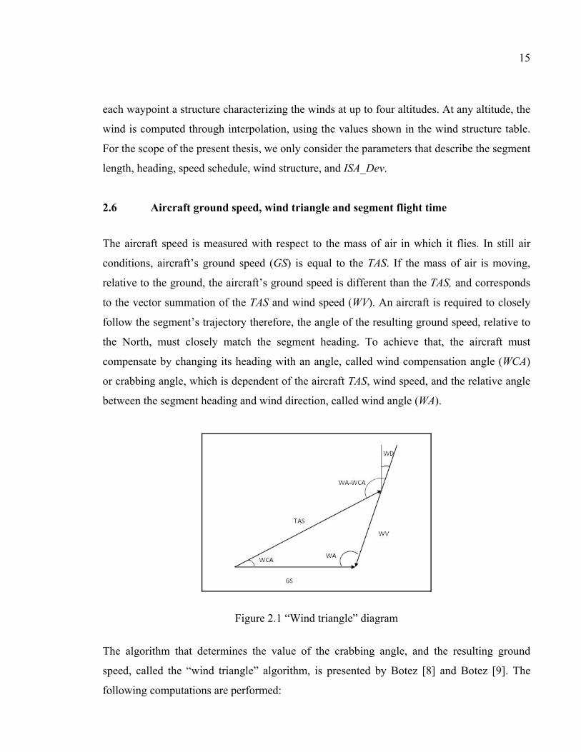
2.6 Aircraft ground speed, wind triangle and segment flight time

The aircraft speed is measured with respect to the mass of air in which it flies. In still air

conditions, aircraft’s ground speed (GS) is equal to the TAS. If the mass of air is moving,

relative to the ground, the aircraft’s ground speed is different than the TAS, and corresponds

to the vector summation of the TAS and wind speed (WV). An aircraft is required to closely

follow the segment’s trajectory therefore, the angle of the resulting ground speed, relative to

the North, must closely match the segment heading. To achieve that, the aircraft must

compensate by changing its heading with an angle, called wind compensation angle (WCA)

or crabbing angle, which is dependent of the aircraft TAS, wind speed, and the relative angle

between the segment heading and wind direction, called wind angle (WA).

Figure 2.1 “Wind triangle” diagram

The algorithm that determines the value of the crabbing angle, and the resulting ground

speed, called the “wind triangle” algorithm, is presented by Botez [8] and Botez [9]. The

following computations are performed:

16

If the relative wind angle, between the segment heading and the wind direction is 0º or 180º,

the crabbing angle is 0º, and the ground speed is:

GS TAS WV= (2.18)

where the “-“ sign corresponds to head winds (wind angle = 0º), and “+” corresponds to tail

winds (wind angle = 180º).

If the relative wind angle is different than 0 or 180º, the ground speed and crabbing angle are

computed using the next equations:

( )arcsin sin *WV

WCA WATAS

=

(2.19)

(Botez, [9], page 28)

( )( )

sin*

sin

WA WCAGS TAS

WA

−=

(2.20)

(Botez, [9], page 29)

It is noted that for a given speed schedule, and wind structure, the TAS and the wind speed

are changing with the altitude. That means that the crabbing angle and the ground speed are

dependent of the flying altitude. Consequently, the segment flight time, computed as the

quotient of the segment length and ground speed, is also dependent of the flying altitude.

17

2.7 Aircraft gross weight and center of gravity position

The aircraft’s gross weight (gw) represents the total weight of the aircraft and is computed as

the sum of the zero fuel gross weight (zfgw), and the fuel weight (fuel), as seen in Federal

Aviation Administration [10]. The zfgw includes the weight of the aircraft’s structure and

payload, that is applied at a specific location, along the longitudinal axis of the aircraft, and

depends on the mass distribution of the structural elements of the aircraft and payload. The

parameter that describes the position is the zero fuel center of gravity position (zfwcg), and

can be expressed as the distance, in inches or millimeters, from the aircraft’s center of gravity

reference point, or in percentage of the Mean Aerodynamic Chord length (MAC). The

aircraft’s center of gravity reference point is the point used as a reference in all center of

gravity computations. It can be located at the datum, or at a given location along the

longitudinal axis of the aircraft, defined by its distance (CGREFDIST) from the datum. The

datum is the point on the longitudinal axis of the aircraft, from which all aircraft longitudinal

quantities are defined.

As zfgw, and fuel weight are applied at different locations than the center of gravity reference

point, each of them will produce a corresponding moment. The convention used in moment

calculations, as described in Federal Aviation Administration [10], is that a positive moment

is given by a weight force applied aft of the cg reference point, and negative if is applied

forward of the cg reference point. The aircraft moment (Ma) is produced by the zfgw, and its

magnitude, as a function of the zfgw and zfwcg, is described through charts or data tables.

The fuel weight generates the fuel moment (Mf). Its magnitude is a function only on the fuel

weight, as the location of the fuel tanks, and the fuel mass distribution, function of the fuel

weight, are aircraft design characteristics. The fuel moment is also described through charts

or data tables.

18

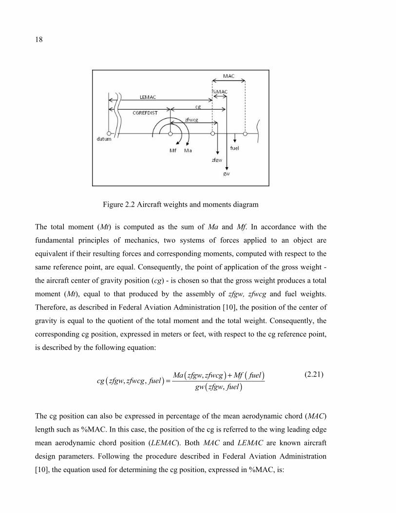
Figure 2.2 Aircraft weights and moments diagram

The total moment (Mt) is computed as the sum of Ma and Mf. In accordance with the

fundamental principles of mechanics, two systems of forces applied to an object are

equivalent if their resulting forces and corresponding moments, computed with respect to the

same reference point, are equal. Consequently, the point of application of the gross weight -

the aircraft center of gravity position (cg) - is chosen so that the gross weight produces a total

moment (Mt), equal to that produced by the assembly of zfgw, zfwcg and fuel weights.

Therefore, as described in Federal Aviation Administration [10], the position of the center of

gravity is equal to the quotient of the total moment and the total weight. Consequently, the

corresponding cg position, expressed in meters or feet, with respect to the cg reference point,

is described by the following equation:

( ) ( ) ( )

( ),

, ,,

Ma zfgw zfwcg Mf fuelcg zfgw zfwcg fuel

gw zfgw fuel

+=

(2.21)

The cg position can also be expressed in percentage of the mean aerodynamic chord (MAC)

length such as %MAC. In this case, the position of the cg is referred to the wing leading edge

mean aerodynamic chord position (LEMAC). Both MAC and LEMAC are known aircraft

design parameters. Following the procedure described in Federal Aviation Administration

[10], the equation used for determining the cg position, expressed in %MAC, is:

19

( )( ) ( )

( )

, ,

,*100

,

cg zfgw zfwcg fuel

Ma zfgw zfwcg Mf fuelCGREFDIST LEMAC

gw zfgw fuel

MAC

=

++ −

(2.22)

2.8 Maximal cruise altitude

The maximal altitude achievable by an aircraft depends, as described by Liden [3], on the

speed, the gross weight, and the altitude (through the effect of the climb fuel burn on the

gross weight) of the aircraft at the time for which the determination of the altitude is made. It

corresponds to the maximal altitude value for which the set of two parameters, the speed

margin, and thrust margin, have values that are zero or positive.

As indicated by Liden [3], the speed margin is computed as the minimum of the difference

between the aircraft’s maximal and schedule speed, and the difference between the aircraft’

schedule and minimal speed. Also, the thrust margin is computed, for a given altitude and

speed schedule, as the difference between the maximum cruise thrust, and the thrust required

to maintain a climb rate of 100 ft/s. The actual parameters used in computing the maximal

and minimal speed, as well as the altitude limitation imposed by the thrust margin are

specific to each aircraft. They are determined by the particular aircraft model used for

defining its corresponding performance tables.

CHAPTER 3

ALGORITHM DEVELOPMENT

The development of a new algorithm, determining the optimal cruise altitude for a constant

speed, level-flight, cruise segment is presented in this chapter. The optimization strategy

chosen for the algorithm is presented first. Subsequently, the algorithm input and output

variables, the structure of the algorithm and its implementation are described.

3.1 The optimization strategy

The critical factor that determined the strategy used in the optimization process is the

requirement that the algorithm is deterministic, i.e. at different instances of time, same input

data produces the same outputs. Therefore, statistical approaches such as meta-heuristic

optimization methods were considered inappropriate from the beginning of the algorithm

development due to their output dependency on factors such as the optimization starting

point, candidate pool choice and size, or limitations imposed by the number of processing

iterations. Consequently, a methodology that uses an analytical approach is chosen, based on

the algorithm described by Liden [3].

3.2 Input variables

The algorithm input variables are divided into four categories: optimization configuration,

aircraft design and performance description, flight segment configuration, and aircraft

configuration. Each category is described in a sub-section of this section:

3.2.1 Optimization configuration parameters

These parameters define the particular conditions for which the optimization is performed.

They are regarded as a set of constant-value algorithm configuration parameters set in

accordance with the airline policy. They correspond to:

22

• the cost index (CI) – in Kg/min;

• optimization distance (OPT_DISTANCE), defining the length of the segment, in Nm;

• minimal cruise altitude (MIN_ALTITUDE), defining the lowest cruise altitude, in ft.

3.2.2 Aircraft design and performance data

The data described in this paragraph represents a subset of general data, specific to each

aircraft, characterizing the aircraft’s geometry, performances, capabilities, and limitations.

The subset is limited to the data used by the optimization algorithm. They are divided into

data specific for an aircraft whose cruise, constant speed, level-flight fuel burn model factors

the cg position and data that is common to all aircraft.

The data specific for an aircraft whose cruise, constant speed, level-flight fuel burn model

factors the cg position are:

• CGREFDIST – the cg reference point position, in meters, from the datum. Only used for

aircraft models that factor the cg position;

• LEMAC – the wing, leading edge mean aerodynamic chord position, in meters, from the

datum. Only used for aircraft models that factor the cg position;

• MAC – the wing, mean aerodynamic length, in meters. Used only for aircraft models that

factor the cg position;

• aircraft moment (Ma) – in kg*m, aircraft performance table describing the aircraft

moment as a function of the zfgw and zfwcg. Used only for aircraft models that factor the

cg position;

• fuel moment (Mf) – in kg*m, aircraft performance table describing the fuel moment as a

function of the fuel weight. Used only for aircraft models that factor the cg position.

The data common to all aircraft are:

23

• ALT_LIMIT – the maximal altitude, in ft, at which the aircraft is allowed to fly, under any

circumstances;

• fuel flow performance tables – one table for each speed mode (ffI for IAS, and ffM for

Mach mode) defining the fuel flow, in Kg/h, as a function of IAS/Mach, gw, ISA_Dev,

and altitude;

• fuel correction factor – a dimensionless parameter, defined as performance tables or

constant values, depending on the aircraft model. If the aircraft model defines it as

performance tables, one table is defined for each speed mode (fcrI for IAS, and fcrM for

Mach mode), as a function of cg, IAS/Mach, gw, and altitude;

• vmo – a constant, or a performance table as a function of altitude, defining the maximal

IAS speed, in Kts;

• mmo – a constant, or a performance table as a function of altitude, defining the maximum

Mach number;

• minspeed – a performance table defining the minimal speed (Mach number), as a function

of the product between the aircraft gross weight (gw) and the density ratio (δ), at the

considered altitude;

• trust margin max_altitude limit – a performance table defining the maximal altitude

limitation due to the thrust margin, in ft. It is described as a function that depends on a

combination of parameters specific to each aircraft that may include the gross weight,

Mach number, cg, and ISA_Dev.

3.2.3 Flight segment configuration

The four parameters corresponding to this category define the characteristics associated with

the cruise flight segment for which the optimization is performed, as follows:

• segment heading (heading), in deg;

• wind structure (wind), defining the wind layers at up to four altitudes. Each layer is

characterized by an altitude – in ft, wind direction (direction) – in degrees, and wind

speed (speed) – in Kts;

24

• speed schedule (schedule), defining the pair of Mach number and IAS. The IAS value is

defined in Kts;

• ISA_Dev, defining the atmosphere standard temperature deviation, in °K.

3.2.4 Aircraft configuration

The aircraft parameters used by the algorithm and described in this section are:

• zfgw – the aircraft zero fuel gross weight, in Kg. Its value is set before take-off and

remains unchanged for the duration of the flight;

• zfwcg – the zero fuel weight center of gravity position, in %MAC. Used only for the

aircrafts whose fuel burn model considers the cg position. Its value is set before take-off

and remains unchanged for the duration of the flight;

• fuel – the fuel weight, in Kg. Its value decreases constantly as the fuel is burned at a fuel

burn rate (fbr) that depends on the aircraft configuration and flight conditions;

• current altitude – the aircraft altitude, in ft, at the time when the optimal altitude is

requested.

3.3 Output data

The objective of the optimization algorithm is to determine the optimal altitude for flying a

selected constant-speed, level-flight, cruise segment. Consequently, the output data is

represented by the optimal cruise altitude (optimal_alt), in ft. However, due to the fact that

the optimal cruise altitude functionality was not available on the platform used for producing

the validation data, the algorithm proposed in this thesis also provides the values for the

segment flight times, fuel burns, and total costs – corresponding to the set of valid cruise

altitudes. This facilitates the evaluation of the performances of the new fuel burn computing

algorithm.

25

3.4 Algorithm processing steps

The algorithm follows the general processing steps as presented by Liden [3]. They are:

• determining the set of cruise altitudes used in the process of optimization;

• computing the flight time at each altitude in the set of cruise altitudes;

• computing the fuel burn at each altitude in the set of cruise altitudes;

• computing the total cost at each altitude in the set of cruise altitudes;

• determining the altitude yielding the minimal cost.

These steps rely on auxiliary functions that perform general tasks such as: IAS, and Mach to

TAS conversion, ground speed, and cg computing, interpolation, and numerical integration.

3.5 Algorithm implementation

Having chosen the type of algorithm employed (analytical) and knowing the number and

order of the computing steps used for determining the optimal altitude, the implementation

addresses two principal objectives: first, an algorithm computing the fuel burn, that accounts

for the continuous variation of the fuel burn rate with the gross weight (and cg); second, the

computations will be performed in a manner that is compatible with the algorithm’s response

time requirements.

Analyzing the set of algorithm input parameters, it can be observed that they can be

regrouped in three categories:

1) Parameters that have a constant value for the duration of the flight - zfgw, zfwcg, CI,

OPT_DISTANCE, MIN_ALTITUDE, as well as the aircraft performance and design

data.

2) Variables whose values may change, but at longer intervals of time such as the speed

schedule (IAS, Mach), ISA_Dev, segment heading, and wind structure - and they are

considered constant on the segment for which the optimal altitude is computed.

26

3) Variables whose values are changing constantly under the influence or as a consequence

of the fuel burn – i.e. the fuel, and thus the gw and cg.

It can be noted that certain computations can only be performed at the time at which the

determination of the optimal altitude is requested, as they are dependent on aircraft’s gross

weight and cg. These computations refer to: maximal altitude, the fuel burn and the total cost,

for each altitude in the determined range of acceptable cruise altitudes. However, certain

computations that depend only on parameters that belong to categories 1) and 2), above, can

be performed upon a parameter value’s modification, and the results used in all subsequent

computations. One such example is the generation of IAS to TAS and Mach to TAS

conversion tables. The modules implementing different parameter calculations are described

in the next sub-sections.

3.5.1 TAS and crossover altitude module

This module is executed at each modification of the speed schedule. It pre-computes the IAS

to TAS and Mach to TAS conversion tables, and the crossover altitude, for the set of altitudes,

multiple of 1000ft., situated between the MIN_ALTITUDE and ALT_LIMIT. The module

ensures that valid TAS values are available for any given speed schedule and cruise altitude

range.

The IAS to TAS conversion is performed using equations (2.15) and (2.16), and the Mach to

TAS conversion is performed using equation (2.17). The corresponding parameters of the

standard atmosphere, used in this thesis, are those presented in Appendix B of Asselin, [7].

The crossover altitude is detected, by comparing the two sets of TAS values, as the altitude at

which the TAS(Mach) equals the TAS(IAS).

27

3.5.2 The maximal cruise altitude and cruise altitude range module

This module computes the range of valid cruise altitudes, corresponding to the aircraft’s

status at the initial point of the cruise segment for which the optimal altitude is determined. It

is executed upon each optimal altitude request.

For each altitude, multiple of 1000ft., situated between MIN_ALTITUDE and ALT_LIMIT,

it computes the following parameters:

• The TAS_min(altitude), the TAS corresponding to the Mach number computed from the

minspeed interpolation table, function of the gw, and the pressure ratio at the evaluated

altitude, δ(altitude).

• The vmo_TAS(altitude), and mmo_TAS(altitude) corresponding to the vmo and mmo

aircraft performance parameters/ interpolation tables.

It then compares these values with the aircraft TAS(altitude), computed from the speed

schedule (IAS or Mach, function of the position of the crossover altitude value). The

speed_limited_altitude is the highest altitude at which TAS(altitude) is larger than

TAS_min(altitude), and smaller than vmo_TAS(altitude) and mmo_TAS(altitude). Then, it

computes the max_thrust_altitude, from the trust margin max_altitude limit performance

table, as a function of a combination of gross weight, Mach number, cg, and ISA_Dev

parameters, depending on the aircraft model.

The maximal cruise altitude is computed as the minimum between the speed_limited_altitude

and the max_thrust_altitude. Consequently, the range of valid cruise altitudes is composed of

the altitudes, multiples of 1,000 ft., situated between the MIN_ALTITUDE and maximal

cruise altitude.

28

3.5.3 Ground speeds and segment flight times

This module is executed upon each request for the optimal altitude. First, it computes the

ground speed for each altitude, multiple of 1,000 ft. in the range of valid cruise altitudes. For

still air conditions, the ground speed at any altitude, is equal to TAS at that same altitude. For

constant wind conditions, the ground speed, at any altitude, is computed in two steps. First,

the wind parameters (direction and speed) are determined from the wind table associated

with the cruise segment, through linear interpolation. Subsequently, the ground speed is

computed using the “driftcorr” MATLAB function, implementing the “wind triangle”

algorithm. The arguments passed to the “driftcorr” function are: the TAS, cruise segment

heading, wind direction and wind speed. Finally, the cruise segment flight time, at each

altitude is computed by dividing the cruise segment’s length (OPT_DISTANCE), to the

ground speed at the corresponding altitude.

3.5.4 The fuel burn

The actual fuel burn value can only be computed at the moment of the request for the optimal

altitude, due to its dependency on the gw (and cg). More, computing the fuel burn,

considering the continuous variation of the gw (and cg) along the cruise segment, requires

two elements: Firstly, expressing the fbr as a function of time. Secondly, performing the

integration of the, time dependent, fbr function, on a time domain corresponding to the

segment flight time. The integration is a time, and computing resources demanding process. It

becomes apparent that meeting the response time requirements cannot be achieved by

performing all fuel burn computations at the moment of the optimal altitude request.

Therefore, the method presented in this thesis performs the computations in steps, at different

times. It takes into account two facts: first, aircraft performances are defined through linear

interpolation tables; second, the rate of variation of each of the variables, that determine the

fuel burn rate, corresponds to one of the three categories presented in the beginning of the

section 3.5. It means that there is a set of values for each variable associated with the input of

the interpolation tables that defines linearity domains for the output, interpolated, variable.

29

This propriety is used in finding the time-dependent expression of the fuel burn function,

fbr(t). It also means that we can decompose the fuel burn computations in three sub-modules

(steps), corresponding to the three categories of variables.

The implementation of the algorithm is function of the fuel burn aircraft model used – cg

dependent or cg independent. As presented in sub-section 3.2.2, two sets of fuel flow and fuel

correction factor performance tables are defined, one for each type of cruise speeds - IAS or

Mach. Since the difference between the two sets of tables refers only to the type of the speed,

the computations associated with each set are identical. Consequently, the implementation of

the fuel burn computation algorithm is described only for the Mach index speeds as for the

IAS the algorithm is identical.

The algorithm is composed of three modules as follows:

• An initialization module, executed before take-off, once the aircraft zfgw,(zfwcg) and fuel

values are set. A series of auxiliary tables are built and subsequently used by the next two

modules.

• The intermediary module, that builds IAS and Mach-based fuel burn look-up tables that

describe the dependency between the initial gw, IAS/Mach, ISA_Dev, the cruise altitude,

the flight time, and the final gw, thus the fuel burn. The module is executed each time the

speed schedule or ISA_Dev parameters change, or as required by the update strategy. The

tables are generated for altitudes situated between MIN_ALTITUDE and ALT_LIMIT.

• The fuel burn module, extracting the fuel burn quantity as a function of the gw at the

initial point of the cruise segment, the evaluated cruise altitude, and the corresponding

flight time. It is executed, at each request for the optimal altitude, a number of times

equal to the pre-determined number of valid cruise altitudes.

3.5.4.1 The initialization module

The main goal of this module is to determine the set of gross weight values, {gwi}, for which

every interval [gwi, gwi+1] maps linearity domains in all performance interpolation tables

30

used in the fuel burn rate computation. For the cg independent model, the module only

identifies and assembles the gw values defined in the ffI, and ffM performance tables.

For the cg dependent model however, the gw values explicitly, or implicitly, defined by the

fcrI, fcrM, and Mf performance tables are also considered. First, it determines the set of {gwj}

values, explicitly defined in the fcrI and fcrM tables. Then, a new fuel moment table as a

function of gw, Mfgw(gw) is generated. The input variable, fuel, is replaced by the

corresponding gross weight:

k kgw zfgw fuel= + (3.1)

Subsequently, the set of gw values, {gwp} is determined, that corresponds to the cg values

defined in the fcr tables. As Mfgw(gw) is defined as a linear interpolation table, on each

domain [gwk, gwk+1] the rate of variation of the fuel moment is constant. Its value is computed

using the next equation:

( ) ( )1

1k

fgw fgw k fgw k

k kgw

M M gw M gw

gw gw gw+

+

∂ −=

∂ −

(3.2)

Consequently, the value of the fuel moment corresponding to a gross weight in the domain

[gwk, gwk+1] is computed using the equation:

( ) ( )1 1* *

k k

fgw fgwfgw fgw k k

gw gw

M MM gw M gw gw gw

gw gw+ +

∂ ∂= − +

∂ ∂

(3.3)

By expressing, in equation (2.22), the fuel moment function of the gw, using the Mfgw(gw),

the equation describing the cg function of the gw becomes:

31

( )

( ) ( ),*100a fgwM zfgw zfwcg M gw

CGREFDIST LEMACgw

cg gwMAC

+ + −

=

(3.4)

Consequently, on a gross weight domain, the gross weight value corresponding to a given cg

position can be computed by replacing Mfgw(gw) given by equation (3.3) into equation (3.4):

( )( ) ( )1 1, *

*100

k

k

fgwa fgw k k

gw

fgw

gw

MM zfgw zfwcg M gw gw

gwgw cg

Mcg MACCGREFDIST LEMAC

gw

+ +

∂ + − ∂ = ∂ − + − ∂

(3.5)

Therefore, the set of gross weight values, {gwp}, is computed using equation (3.5), by

evaluating each cg value defined by the fcr tables, on all [gwk, gwk+1] gross weight domains.

A gwp thus computed is considered valid, and retained, if its value lies within the gross

weight domain on which it was computed. Finally, the {gwk}, {gwj} and {gwp} sets are added

to the initial set of {gwi} values:

{ } { } { } { } { }i i j k pgw gw gw gw gw= (3.6)

This new set of gross weight values {gwi} ensures that each domain [gwi, gwi+1] corresponds

to gw and cg linearity domains, in all performance interpolation tables used for computing

the fuel burn rate. Next, the Mfgw table is rebuilt according to the new set of {gwi} values.

Two more auxiliary tables, used by the intermediary module, are built for the same set of

{gwi} values. First, the CG_AT_GW(gwi) table, storing the cg position, corresponding to each

gw in the {gwi} set, is computed using equation (3.4). The second table, called

CG_SLOPE(gwi), stores, for each domain [gwi, gwi+1], a coefficient that is used to determine

the cg variation (dcg) function of the gross weight variation (dgw), where both are referenced

to their corresponding value at gwi+1. To determine the equation used to compute the

elements of the table we are using the next equation:

32

( ) ( ) ( )1idcg gw cg gw cg gw+= − (3.7)

In equation (3.7), replacing the cg values with the values given by equation (3.4), and

subsequently Mfgw(gw) with equation (3.3), we obtain:

( )( ) ( )1 1

1

100* ,

*

1 1

i

fgwa fgw i i

gw

i i

MM zfgw zfwcg M gw gw

gwdcg gw

MAC

gw gw

+ +

+

∂ + −

∂ =

−

(3.8)

Denoting:

1idgw gw gw+= − (3.9)

and

( )( ) ( )1 1

1

100* ,

_*

i

fgwa fgw i i

gw

ii

MM zfgw zfwcg M gw gw

gwCG SLOPE gw

MAC gw

+ +

+

∂ + −

∂ =

(3.10)

the equation (3.8) can be written as a function of dgw, therefore it becomes:

( )

1

_ ( )*ii

dgwdcg dgw CG SLOPE gw

gw dgw+

= −

(3.11)

33

3.5.4.2 The intermediary module

This module constructs, for a given speed schedule, and ISA_Dev, a structure describing the

relationship between the aircraft’s initial gw, the cruise altitude, the flight time, and the final

gw. The data is assembled for a number of altitudes, multiples of 1,000 ft, situated between

the MIN_ALTITUDE and ALT_LIMIT. The IAS or Mach performances are characterized,

depending on the corresponding altitude position relative to the crossover altitude. At each

altitude, the fuel burn data is generated for a number of gross weight domains that depend on

the structure’s update strategy, and the OPT_DISTANCE. It should cover, at least, the fuel

burn that can occur on flying the cruise segment, under any conditions. The implementation

considers the generation of the fuel burn data for the entire set of gross weight domains,

starting with the one containing the gw value at the time the data is generated, further to the

gw corresponding to fuel = 0. It allows the investigation of the module’s response time

performance, as a function of the gross weight range.

The present paragraph describes the computations performed for Mach index speeds, at a

given altitude on a gross weight domain [gwi, gwi+1], for cg dependent and cg independent

aircraft models. At IAS speeds, the computations are identical, but are using the IAS

performance interpolation tables (ffI, and fcrI). First, the fuel burn rate (fbr) equation,

function of the dgw, is developed using the equation of the linear interpolation. Then the

equation is rewritten, to describe the fbr variation function of time. Finally, the time-

dependent fbr function is integrated using the Runge-Kutta 4 (RK4) algorithm, as described

by Butcher [11].

The fuel burn rate (fbr) is computed as the product between the fuel flow (ff) and the fuel

correction factor (fcr). The steps needed for its calculation are shown next. Denoting:

( )1 1, , _ ,M iff ff Mach gw ISA Dev altitude+= (3.12)

and

34

( )2 , , _ ,M iff ff Mach gw ISA Dev altitude= (3.13)

the value of the fuel flow, at a gross weight described by the dgw, is computed by linear

interpolation, using the equation:

( ) 1 21

1i i

ff ffff dgw ff dgw

gw gw+

−= −−

(3.14)

Denoting:

0 1A ff= (3.15)

and

1 21

1i i

ff ffA

gw gw+

−=−

(3.16)

the equation (3.14) becomes:

( ) 0 1 *ff dgw A A dgw= − (3.17)

For the cg independent aircraft model and Mach index speeds, the fuel correction factor fcrM

is a constant value. Therefore, denoting C0 = fcrM, the equation of the fuel burn rate as a

function of the dgw is:

( ) ( )0 0 1 *fbr dgw C A A dgw= − (3.18)

Observing that the dgw changes with time, as the fuel is burned, the fbr variation is described

as a function of time:

35

( ) ( )( )0 0 1 *fbr t C A A dgw t= − (3.19)

There is also a direct relationship between dgw(t) and fbr(t), as the gross weight variation is

produced as a result of burning the fuel at a rate described by the fbr(t). Consequently, the

equation that connects dgw and fbr is:

( ) ( )dgw t fbr t dt= (3.20)

Denoting dgw(t) = I implies that fbr(t) = dI/dt. Therefore, equation (3.19) becomes:

( )0 0 1 *dI

C A A Idt

= − (3.21)

This differential equation describes the gross weight variation (dgw) as a function of the

flight time, on a gross weight domain [gwi, gwi+1], for the cg independent aircraft model.

For the cg dependent aircraft model, for Mach index speeds, the fuel correction factor (fcr) is

obtained from the fcrM interpolation table. We denote:

( )( )( )( )( )( )( )( )

11 1 1

12 1

21 1

22

_ _ , , ,

_ _ , , ,

_ _ , , ,

_ _ , , ,

M i i

M i i

M i i

M i i

cr fcr CG AT GW gw Mach gw altitude

cr fcr CG AT GW gw Mach gw altitude

cr fcr CG AT GW gw Mach gw altitude

cr fcr CG AT GW gw Mach gw altitude

+ +

+

+

=

=

=

=

(3.22)

Interpolating, along the gw input parameter of the fuel correction factor performance table,

leads to the equations:

36

11 211 11

1

12 222 12

1

i i

i i

cr crfcr cr dgw

gw gw

cr crfcr cr dgw

gw gw

+

+

−= −−−= −−

(3.23)

Subsequently, interpolating between the values of fcr1 and fcr2, to account for the variation of

the cg, with respect to cgi+1 = cg(gwi+1), leads to:

( ) ( )1 2

11i i

fcr fcrfcr fcr dcg

cg gw cg gw+

−= −−

(3.24)

Replacing the terms of equation (3.24), with their definitions given in equations (3.11),(3.22)

and (3.23), and denoting:

( ) ( )

( ) ( )

0 11 1

11 1211 211 11 1

1 1

11 12 21 222 11 21

1 1

0 1

_

_ _ ( ) _ _ ( )

_1

_ _ ( ) _ _ ( )

i

ii

i i i i

i

i i i i

i

B cr gw

cr cr CG SLOPE gwcr crB cr gw

gw gw CG AT GW gw CG AT GW gw

cr cr cr cr CG SLOPE gwB cr cr

gw gw CG AT GW gw CG AT GW gw

C gw

+

++ +

+ +

+

=−−= + +

− −

− − + = − + − − =

(3.25)

the equation describing fcr(dgw) becomes:

( )

20 1 2

0

* *B B dgw B dgwfcr dgw

C dgw

− +=−

(3.26)

Consequently, the equation describing the fbr(dgw), for the cg dependent aircraft model, is:

( ) ( )( )2

0 1 0 1 2

0

* * *A A dgw B B dgw B dgwfbr dgw

C dgw

− − +=

−

(3.27)

37

Considering equation (3.20) and denoting dgw(t) = I implies that fbr(t) = dI/dt. Replacing the

dgw(t) and fbr(t) in equation (3.27) leads to the time dependent differential equation:

( )( )20 1 0 1 2

0

* * *A A I B B I B IdI

dt C I

− − +=

−

(3.28)

For each gross weight domain, and altitude, a look-up table describing the gross weight

variation with time is produced by integration of equation (3.21), or (3.28), depending on the

aircraft modeling, using the RK4 numerical integration algorithm. The gross weight

information stored in the look-up table corresponds to time instances, multiples of the

integration time step value, referenced to the beginning of the gross weight domain.

Therefore, searches in the look-up table can be performed depending on the gross weight, or

the flight time.

The Runge-Kutta numerical integration is performed using the “ode45” MATLAB function.

The integration time step was chosen as the minimum between 30sec and the time required to

burn the entire quantity of fuel corresponding to the gross weight domain. In order to

facilitate the fuel burn computations by the fuel burn module, the time required to burn the

entire quantity of fuel corresponding to the gross weight domain is also stored in the fuel-

burn look-up table.

3.5.4.3 The fuel burn module

The fuel burn module computes fuel burn values, at a given altitude, as the difference

between the value of the gross weight, at the beginning of the considered cruise segment, and

the value of the gross weight after flying for a period equal to the cruise segment’s flight

time. The gross weight domain containing the aircraft’s gross weight value, at the beginning

of the cruise segment, is identified. Subsequently, the corresponding time offset, from the

domain’s initial gross weight is determined. By subtracting it from the gross weight domain’s

total time, the flight time required to reach the domain’s final gross weight is determined.

38

Then, a series of iterations are performed on successive gross weight domains, starting with

the initial domain. Upon each iteration, the flight time corresponding to the selected domain

and the cruise flight time are compared. If the domain’s flight time is smaller, its value is

subtracted from the cruise flight time, and the processing advances to the next iteration,

corresponding to the next gross weight domain. If the domain’s flight time is larger, the final

gross weight is computed as the value corresponding to the time offset, from the beginning of

the domain, equal to the value of the cruise flight time. The fuel burn is then computed as the

difference between the initial and the final gross weight.

3.5.5 The total cost

The total cost (CTOT), expressed in kilograms of fuel, is computed for each altitude in the set

of valid cruise altitudes, using equation (2.6). The value of the integral term is retrieved from

the look-up table using the code implementing the fuel burn module.

3.5.6 The optimal altitude module

The optimal altitude module provides the functionality that represents the main object of the

present thesis. It is executed upon each optimal altitude request and implements the

processing steps described in the sub-section 3.4. It relies on the functions and data provided

by the modules described in sub-section 3.5.1 to 3.5.5, to compute the total cost and fuel burn

for each altitude in the range of valid cruise altitudes.

Subsequently, the optimal altitude is selected as the altitude yielding the minimal cost. If two

or more altitudes present the same minimal cost, the altitude also yielding the minimal fuel

burn is selected as the optimal altitude. If two or more altitudes yield the minimal cost and

minimal fuel burn, the selected altitude corresponds to that closest to the aircraft’s altitude at

the time the optimal altitude is computed.

CHAPTER 4

ALGORITHM VALIDATION

The algorithm was implemented for three aircraft models: Airbus A310, Lockheed L1011,

and Sukhoi RRJ. The validation strategy adopted for each of the three models depended upon

the particularities of the corresponding test platform provided by our research partner CMC

Electronics – Esterline. It is important to note that the validation was not intended, in any

way, to characterize the PTT’s or aircraft’s cruise performances. Such an endeavor requires a

significant amount of time and resources and was already performed as a part of each

product’s certification processes.

The algorithm’s code was developed in MATLAB, and executed on a Microsoft XP - based,

PC platform. For the Airbus A310 and Sukhoi RRJ aircrafts, the main validation data was

produced on a test platform, composed of a PC-based FMS simulator, the CMA9000 PTT,

replicating the CMC Electronics –Esterline CMA9000 FMS. As the optimal altitude

function, implemented by the algorithm described in this thesis, was not available on the test

platform, the optimal altitude validation data was computed using the main validation data

(segment flight times and fuel burns), generated by the CMA9000 PTT. The Lockheed

L1011 validation platform also included a Flightsim 9.1-based aircraft simulator capable of

flying the flight plan programmed on the PTT. The aircraft simulator allowed the recording

of the variation with time of different aircraft parameters, including the aircraft’s gross

weight.

All tests were performed for cruise segments of 500 Nautical miles (399.59Nm for L1011),

corresponding to approximately 1 hour of flight. For the A310 and RRJ models the validation

followed three objectives. The first objective of the validation was the comparison of the

optimal altitude computed by the algorithm with the optimal altitude computed using the

flight times and fuel burns produced by the PTT. The second objective was the evaluation of

the performances of the fuel burn computing algorithm. The third objective was the

40

investigation of the execution times of each of the three modules implementing the

algorithm. For the L1011 model the objective of the validation was the evaluation of the fuel

burn algorithm performances by comparison with the values computed by the PTT and the

Flightsim 9.1 at the optimal altitude computed by the algorithm. This was a limitation

determined by the time required to obtain the Flightsim validation data at one altitude (the

cruise segment’s flight time).

The number of test cases that were evaluated was limited by the time and human resources

available for generating the validation data. Each test was generated manually, i.e. platform

configuration and data retrieval for each altitude, and each test case, required user

intervention. Even without such limitations, an extensive investigation of the algorithm

performances would have been impractical, due to the large number of possible combinations

of the input parameters (IAS and Mach index speeds, wind structure, standard temperature

deviation, zero fuel gross weight, zero fuel weight center of gravity position, fuel weight,

minimal cruise altitude, the optimization distance, cruise segment’s heading and cost index).

While each of the above mentioned input parameters has an influence on the final value of

the optimal altitude, the nature of their influence is not the same.

For instance, cruise segment heading and wind structure are only relevant for constant wind

conditions, through the relative wind angle’s influence on ground speed and segment flight

time. Also, the standard temperature deviation influences the optimal altitude through the

fuel burn rate, hence the fuel burn. However, the evaluation of the algorithm performances

for still air conditions and one value of the ISA_Dev provided valid data related to the fuel

burn and optimal altitude modeling. For these reasons, all test cases considered a cruise

segment heading of 0 deg (North), still air and a standard temperature deviation, ISA_Dev,

equal to 0°K. The value of the optimal altitude was influenced by the minimal cruise altitude

by means of the number of evaluated cruise altitudes. In order to determine the values

describing algorithm modules’ maximal (worst) execution times, all test cases considered a

minimal cruise altitude value of 20,000ft. For example, for the A310 these values were

obtained by generating fuel burn look-up tables for 21 altitudes, and performing cost

evaluations of up to 21 altitudes.

41

According to CMC Electronics, the pair of IAS and Mach values defining a cruise segment’

speed schedule are linked by the following rule: the IAS value of 280 Kts is paired with a

Mach value of 0.78; subsequently, an IAS variation of 20 Kts corresponds to a Mach

variation of 0.02.

For the A310 and RRJ models, the algorithm performances were evaluated for a set of cost

index values equal to 0, 15, 35, 50, and 100. Upon analysis of the algorithm and its validation

data it was found that a difference existed between the flight times computed by the

algorithm and PTT, respectively, that may be explained by two main factors. The first factor

refers to differences in code implementation and data processing due to platform differences.

The second factor relates to the way in which the cruise segment is processed. The PTT

decomposes the cruise segment in a number of sub-segments, of up to a predetermined

length, required by their respective fuel burn computing algorithm. It then computes the total

flight time, and the total fuel burn, as the sum of the sub-segments’ flight times, and fuel

burns respectively. For the tests performed on the PTT, the cruise sub-segments’ length was

set at 50 Nm for A310 and 99.99 Nm for RRJ. On the contrary, the algorithm presented in

this thesis computes the segment flight times and the fuel burns for the entire segment

independently of its length.

As the segment flight time is a parameter that influences both the fuel cost, and the non fuel

cost, a second version of the algorithm was developed, that computed the optimal altitude,

fuel burn and total cost, using the cruise altitude range and corresponding segment flight

times computed by the PTT platform. Thus a better analysis of the optimal altitude, and fuel

burn is obtained, where the differences are specific to the fuel burn computing algorithm

only. The second algorithm was evaluated for the same set of test configurations, and cost

index values. The results of the first algorithm, identified as “Algorithm 1”, and the results of

the second algorithm, identified as “Algorithm 2”, are presented side by side.

42

The execution times of each of the three main modules: initialization, intermediary and

optimal altitude module were measured using the “tic” and “toc” MATLAB functions.

The results corresponding to each of the two developed algorithms describe the algorithm

performances from two perspectives, as follows:

1) Algorithm performances, characterized by:

a) The difference between the optimal altitude computed by the algorithm and the

corresponding optimal altitude computed using the PTT validation data.

b) The relative difference between the flight time, fuel burn and total cost values

computed by the algorithm at the optimal altitude computed by the algorithm, and at

the optimal altitude computed using the PTT validation data, respectively.

c) The relative difference between the flight time, fuel burn and total cost values

computed by the algorithm and the values computed using the PTT validation data,

respectively, at the optimal altitude computed by the algorithm.

2) Algorithm execution time, for each of the three algorithm modules: initialization,

intermediary and optimal altitude.

For the L1011 model, the aircraft’s zfgw and fuel weight, thus gw, at the initial point of the

cruise segment along with the corresponding cruise segment’s flight time, computed by the

PTT, were used for determining the fuel burn values computed by the Flightsim and the

algorithm. Using the PTT-computed flight time was important for two reasons: firstly, the

Flightsim cannot provide the data correlating the flight time and aircraft position relative to

the PTT flight plan. Consequently, as the aircraft’s gw (therefore the fuel weight) data

recorded by the Flightsim is function of the flight time, it is impossible to extract the

information related to the fuel burn function of the aircraft’s position along the cruise

segment; secondly, this allows to compare the PTT, Flightsim and algorithm fuel burn values

for identical flight conditions, therefore, emphasizing the differences that are caused by the

fuel burn computing model only. For the L1011 tests, the PTT cruise sub-segments’ length

was set at 99.99 Nm.

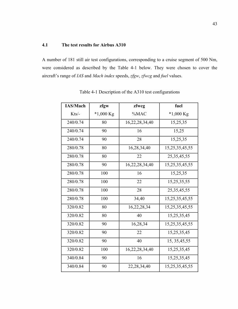
43

4.1 The test results for Airbus A310

A number of 181 still air test configurations, corresponding to a cruise segment of 500 Nm,

were considered as described by the Table 4-1 below. They were chosen to cover the

aircraft’s range of IAS and Mach index speeds, zfgw, zfwcg and fuel values.

Table 4-1 Description of the A310 test configurations

IAS/Mach

Kts/-

zfgw

*1,000 Kg

zfwcg

%MAC

fuel

*1,000 Kg

240/0.74 80 16,22,28,34,40 15,25,35

240/0.74 90 16 15,25

240/0.74 90 28 15,25,35

280/0.78 80 16,28,34,40 15,25,35,45,55

280/0.78 80 22 25,35,45,55

280/0.78 90 16,22,28,34,40 15,25,35,45,55

280/0.78 100 16 15,25,35

280/0.78 100 22 15,25,35,55

280/0.78 100 28 25,35,45,55

280/0.78 100 34,40 15,25,35,45,55

320/0.82 80 16,22,28,34 15,25,35,45,55

320/0.82 80 40 15,25,35,45

320/0.82 90 16,28,34 15,25,35,45,55

320/0.82 90 22 15,25,35,45

320/0.82 90 40 15, 35,45,55

320/0.82 100 16,22,28,34,40 15,25,35,45

340/0.84 90 16 15,25,35,45

340/0.84 90 22,28,34,40 15,25,35,45,55

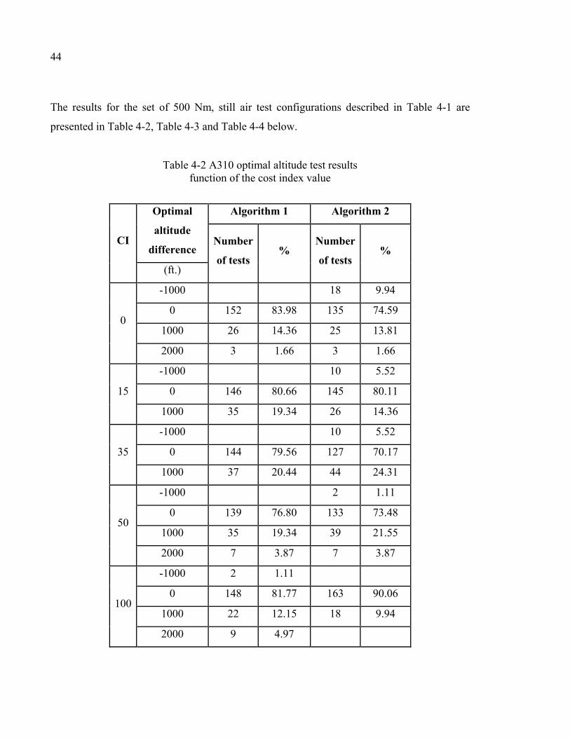
44

The results for the set of 500 Nm, still air test configurations described in Table 4-1 are

presented in Table 4-2, Table 4-3 and Table 4-4 below.

Table 4-2 A310 optimal altitude test results function of the cost index value

CI

Optimal

altitude

difference

Algorithm 1 Algorithm 2

Number

of tests %

Number

of tests %

(ft.)

0

-1000 18 9.94

0 152 83.98 135 74.59

1000 26 14.36 25 13.81

2000 3 1.66 3 1.66

15

-1000 10 5.52

0 146 80.66 145 80.11

1000 35 19.34 26 14.36

35

-1000 10 5.52

0 144 79.56 127 70.17

1000 37 20.44 44 24.31

50

-1000 2 1.11

0 139 76.80 133 73.48

1000 35 19.34 39 21.55

2000 7 3.87 7 3.87

100

-1000 2 1.11

0 148 81.77 163 90.06

1000 22 12.15 18 9.94

2000 9 4.97

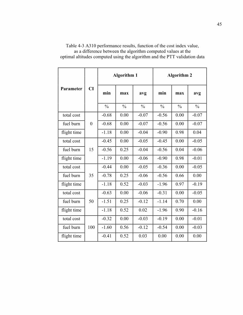
45

Table 4-3 A310 performance results, function of the cost index value, as a difference between the algorithm computed values at the

optimal altitudes computed using the algorithm and the PTT validation data

Parameter CI

Algorithm 1 Algorithm 2

min max avg min max avg

% % % % % %

total cost

0

-0.68 0.00 -0.07 -0.56 0.00 -0.07

fuel burn -0.68 0.00 -0.07 -0.56 0.00 -0.07

flight time -1.18 0.00 -0.04 -0.90 0.98 0.04

total cost

15

-0.45 0.00 -0.05 -0.45 0.00 -0.05

fuel burn -0.56 0.25 -0.04 -0.56 0.04 -0.06

flight time -1.19 0.00 -0.06 -0.90 0.98 -0.01

total cost

35

-0.44 0.00 -0.05 -0.36 0.00 -0.05

fuel burn -0.78 0.25 -0.06 -0.56 0.66 0.00

flight time -1.18 0.52 -0.03 -1.96 0.97 -0.19

total cost

50

-0.63 0.00 -0.06 -0.31 0.00 -0.05

fuel burn -1.51 0.25 -0.12 -1.14 0.70 0.00

flight time -1.18 0.52 0.02 -1.96 0.90 -0.16

total cost

100

-0.32 0.00 -0.03 -0.19 0.00 -0.01

fuel burn -1.60 0.56 -0.12 -0.54 0.00 -0.03

flight time -0.41 0.52 0.03 0.00 0.00 0.00

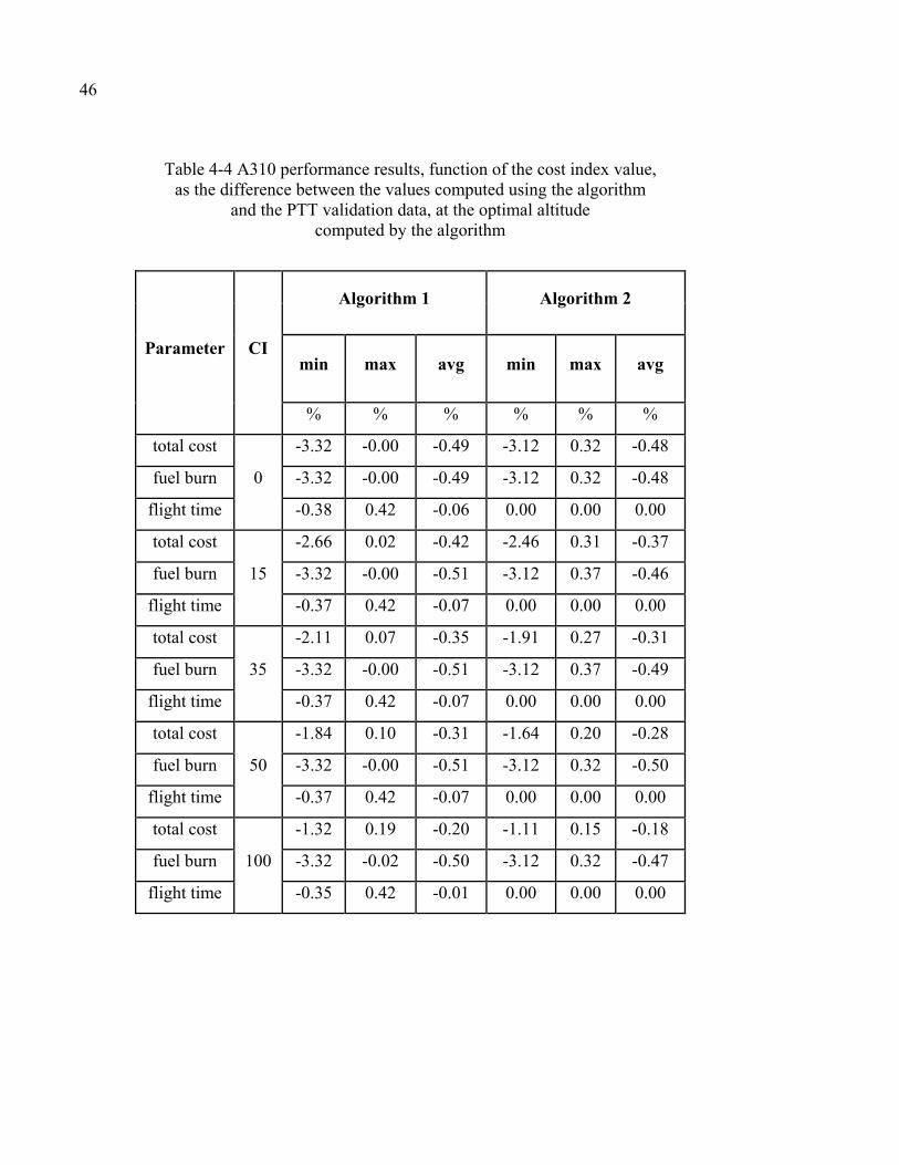
46

Table 4-4 A310 performance results, function of the cost index value, as the difference between the values computed using the algorithm

and the PTT validation data, at the optimal altitude computed by the algorithm

Parameter CI

Algorithm 1 Algorithm 2

min max avg min max avg

% % % % % %

total cost

0

-3.32 -0.00 -0.49 -3.12 0.32 -0.48

fuel burn -3.32 -0.00 -0.49 -3.12 0.32 -0.48

flight time -0.38 0.42 -0.06 0.00 0.00 0.00

total cost

15

-2.66 0.02 -0.42 -2.46 0.31 -0.37

fuel burn -3.32 -0.00 -0.51 -3.12 0.37 -0.46

flight time -0.37 0.42 -0.07 0.00 0.00 0.00

total cost

35

-2.11 0.07 -0.35 -1.91 0.27 -0.31

fuel burn -3.32 -0.00 -0.51 -3.12 0.37 -0.49

flight time -0.37 0.42 -0.07 0.00 0.00 0.00

total cost

50

-1.84 0.10 -0.31 -1.64 0.20 -0.28

fuel burn -3.32 -0.00 -0.51 -3.12 0.32 -0.50

flight time -0.37 0.42 -0.07 0.00 0.00 0.00

total cost

100

-1.32 0.19 -0.20 -1.11 0.15 -0.18

fuel burn -3.32 -0.02 -0.50 -3.12 0.32 -0.47

flight time -0.35 0.42 -0.01 0.00 0.00 0.00

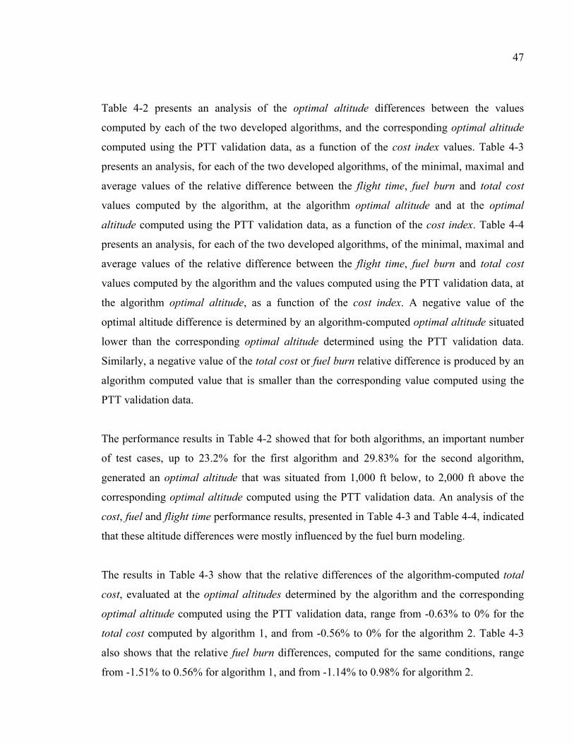
47

Table 4-2 presents an analysis of the optimal altitude differences between the values

computed by each of the two developed algorithms, and the corresponding optimal altitude

computed using the PTT validation data, as a function of the cost index values. Table 4-3

presents an analysis, for each of the two developed algorithms, of the minimal, maximal and

average values of the relative difference between the flight time, fuel burn and total cost

values computed by the algorithm, at the algorithm optimal altitude and at the optimal

altitude computed using the PTT validation data, as a function of the cost index. Table 4-4

presents an analysis, for each of the two developed algorithms, of the minimal, maximal and

average values of the relative difference between the flight time, fuel burn and total cost

values computed by the algorithm and the values computed using the PTT validation data, at

the algorithm optimal altitude, as a function of the cost index. A negative value of the

optimal altitude difference is determined by an algorithm-computed optimal altitude situated

lower than the corresponding optimal altitude determined using the PTT validation data.

Similarly, a negative value of the total cost or fuel burn relative difference is produced by an

algorithm computed value that is smaller than the corresponding value computed using the

PTT validation data.

The performance results in Table 4-2 showed that for both algorithms, an important number

of test cases, up to 23.2% for the first algorithm and 29.83% for the second algorithm,

generated an optimal altitude that was situated from 1,000 ft below, to 2,000 ft above the

corresponding optimal altitude computed using the PTT validation data. An analysis of the

cost, fuel and flight time performance results, presented in Table 4-3 and Table 4-4, indicated

that these altitude differences were mostly influenced by the fuel burn modeling.

The results in Table 4-3 show that the relative differences of the algorithm-computed total

cost, evaluated at the optimal altitudes determined by the algorithm and the corresponding

optimal altitude computed using the PTT validation data, range from -0.63% to 0% for the

total cost computed by algorithm 1, and from -0.56% to 0% for the algorithm 2. Table 4-3

also shows that the relative fuel burn differences, computed for the same conditions, range

from -1.51% to 0.56% for algorithm 1, and from -1.14% to 0.98% for algorithm 2.

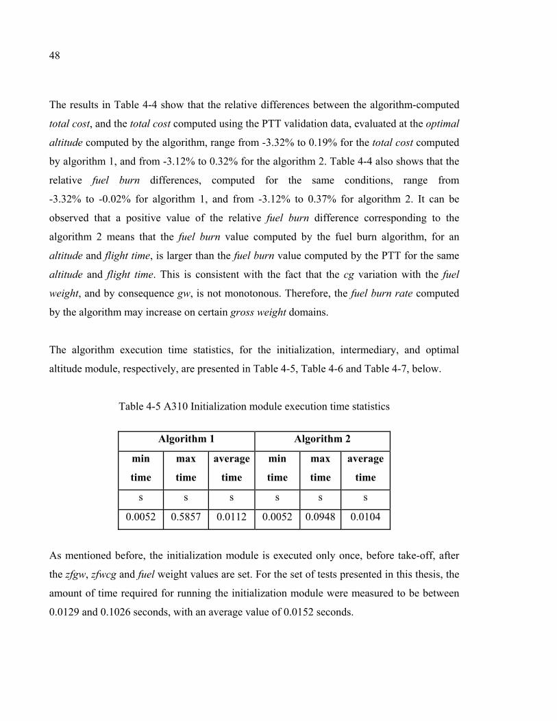
48

The results in Table 4-4 show that the relative differences between the algorithm-computed

total cost, and the total cost computed using the PTT validation data, evaluated at the optimal

altitude computed by the algorithm, range from -3.32% to 0.19% for the total cost computed

by algorithm 1, and from -3.12% to 0.32% for the algorithm 2. Table 4-4 also shows that the

relative fuel burn differences, computed for the same conditions, range from

-3.32% to -0.02% for algorithm 1, and from -3.12% to 0.37% for algorithm 2. It can be

observed that a positive value of the relative fuel burn difference corresponding to the

algorithm 2 means that the fuel burn value computed by the fuel burn algorithm, for an

altitude and flight time, is larger than the fuel burn value computed by the PTT for the same

altitude and flight time. This is consistent with the fact that the cg variation with the fuel

weight, and by consequence gw, is not monotonous. Therefore, the fuel burn rate computed

by the algorithm may increase on certain gross weight domains.

The algorithm execution time statistics, for the initialization, intermediary, and optimal

altitude module, respectively, are presented in Table 4-5, Table 4-6 and Table 4-7, below.

Table 4-5 A310 Initialization module execution time statistics

Algorithm 1 Algorithm 2

min

time

max

time

average

time

min

time

max

time

average

time

s s s s s s

0.0052 0.5857 0.0112 0.0052 0.0948 0.0104

As mentioned before, the initialization module is executed only once, before take-off, after

the zfgw, zfwcg and fuel weight values are set. For the set of tests presented in this thesis, the

amount of time required for running the initialization module were measured to be between

0.0129 and 0.1026 seconds, with an average value of 0.0152 seconds.

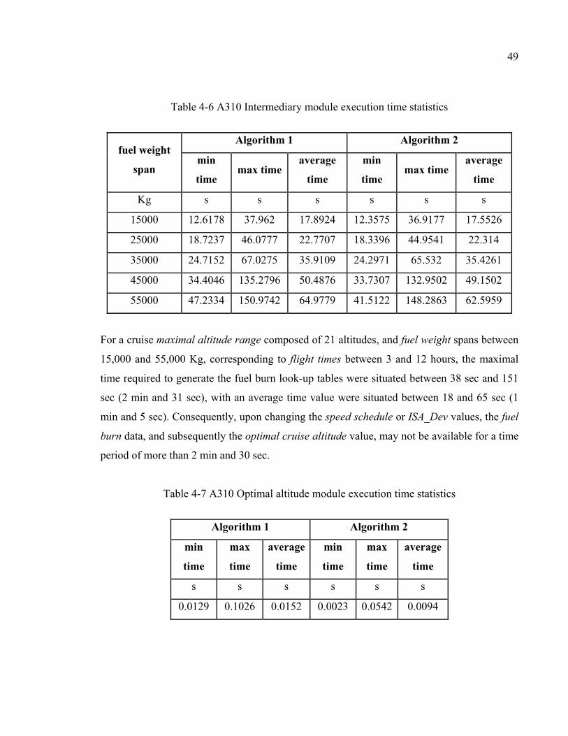
49

Table 4-6 A310 Intermediary module execution time statistics

fuel weight

span

Algorithm 1 Algorithm 2

min

time max time

average

time

min

time max time

average

time

Kg s s s s s s

15000 12.6178 37.962 17.8924 12.3575 36.9177 17.5526

25000 18.7237 46.0777 22.7707 18.3396 44.9541 22.314

35000 24.7152 67.0275 35.9109 24.2971 65.532 35.4261

45000 34.4046 135.2796 50.4876 33.7307 132.9502 49.1502

55000 47.2334 150.9742 64.9779 41.5122 148.2863 62.5959

For a cruise maximal altitude range composed of 21 altitudes, and fuel weight spans between

15,000 and 55,000 Kg, corresponding to flight times between 3 and 12 hours, the maximal

time required to generate the fuel burn look-up tables were situated between 38 sec and 151

sec (2 min and 31 sec), with an average time value were situated between 18 and 65 sec (1

min and 5 sec). Consequently, upon changing the speed schedule or ISA_Dev values, the fuel

burn data, and subsequently the optimal cruise altitude value, may not be available for a time

period of more than 2 min and 30 sec.

Table 4-7 A310 Optimal altitude module execution time statistics

Algorithm 1 Algorithm 2

min

time

max

time

average

time

min

time

max

time

average

time

s s s s s s

0.0129 0.1026 0.0152 0.0023 0.0542 0.0094

50

The optimal altitude module time statistics, presented in Table 4-7, show that for still air

conditions, and a cruise altitude range of 21 altitudes, the execution time were situated

between 13ms and 103ms, with an average value of 15ms.

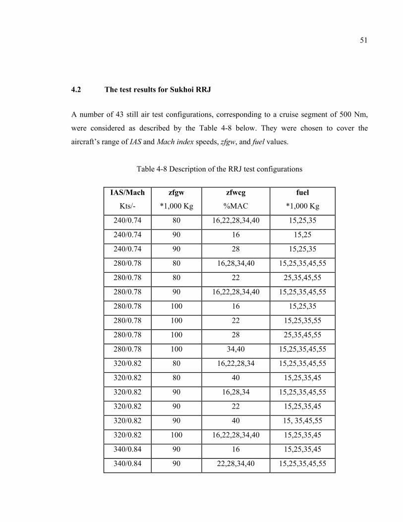
51

4.2 The test results for Sukhoi RRJ

A number of 43 still air test configurations, corresponding to a cruise segment of 500 Nm,

were considered as described by the Table 4-8 below. They were chosen to cover the

aircraft’s range of IAS and Mach index speeds, zfgw, and fuel values.

Table 4-8 Description of the RRJ test configurations

IAS/Mach

Kts/-

zfgw

*1,000 Kg

zfwcg

%MAC

fuel

*1,000 Kg

240/0.74 80 16,22,28,34,40 15,25,35

240/0.74 90 16 15,25

240/0.74 90 28 15,25,35

280/0.78 80 16,28,34,40 15,25,35,45,55

280/0.78 80 22 25,35,45,55

280/0.78 90 16,22,28,34,40 15,25,35,45,55

280/0.78 100 16 15,25,35

280/0.78 100 22 15,25,35,55

280/0.78 100 28 25,35,45,55

280/0.78 100 34,40 15,25,35,45,55

320/0.82 80 16,22,28,34 15,25,35,45,55

320/0.82 80 40 15,25,35,45

320/0.82 90 16,28,34 15,25,35,45,55

320/0.82 90 22 15,25,35,45

320/0.82 90 40 15, 35,45,55

320/0.82 100 16,22,28,34,40 15,25,35,45

340/0.84 90 16 15,25,35,45

340/0.84 90 22,28,34,40 15,25,35,45,55

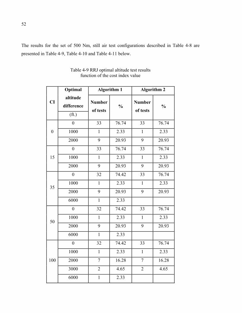
52

The results for the set of 500 Nm, still air test configurations described in Table 4-8 are

presented in Table 4-9, Table 4-10 and Table 4-11 below.

Table 4-9 RRJ optimal altitude test results function of the cost index value

CI

Optimal

altitude

difference

Algorithm 1 Algorithm 2

Number

of tests %

Number

of tests %

(ft.)

0

0 33 76.74 33 76.74

1000 1 2.33 1 2.33

2000 9 20.93 9 20.93

15

0 33 76.74 33 76.74

1000 1 2.33 1 2.33

2000 9 20.93 9 20.93

35

0 32 74.42 33 76.74

1000 1 2.33 1 2.33

2000 9 20.93 9 20.93

6000 1 2.33

50

0 32 74.42 33 76.74

1000 1 2.33 1 2.33

2000 9 20.93 9 20.93

6000 1 2.33

100

0 32 74.42 33 76.74

1000 1 2.33 1 2.33

2000 7 16.28 7 16.28

3000 2 4.65 2 4.65

6000 1 2.33

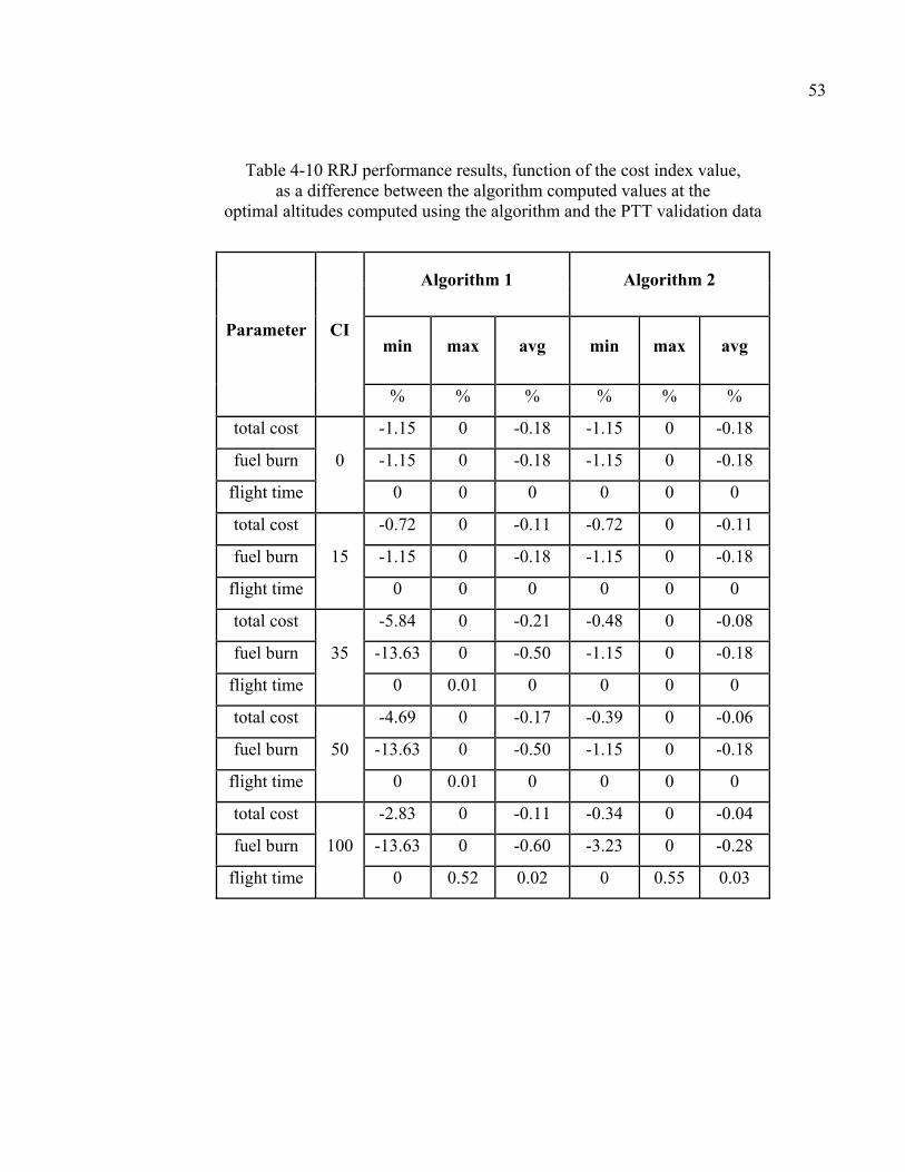
53

Table 4-10 RRJ performance results, function of the cost index value, as a difference between the algorithm computed values at the

optimal altitudes computed using the algorithm and the PTT validation data

Parameter CI

Algorithm 1 Algorithm 2

min max avg min max avg

% % % % % %

total cost

0

-1.15 0 -0.18 -1.15 0 -0.18

fuel burn -1.15 0 -0.18 -1.15 0 -0.18

flight time 0 0 0 0 0 0

total cost

15

-0.72 0 -0.11 -0.72 0 -0.11

fuel burn -1.15 0 -0.18 -1.15 0 -0.18

flight time 0 0 0 0 0 0

total cost

35

-5.84 0 -0.21 -0.48 0 -0.08

fuel burn -13.63 0 -0.50 -1.15 0 -0.18

flight time 0 0.01 0 0 0 0

total cost

50

-4.69 0 -0.17 -0.39 0 -0.06

fuel burn -13.63 0 -0.50 -1.15 0 -0.18

flight time 0 0.01 0 0 0 0

total cost

100

-2.83 0 -0.11 -0.34 0 -0.04

fuel burn -13.63 0 -0.60 -3.23 0 -0.28

flight time 0 0.52 0.02 0 0.55 0.03

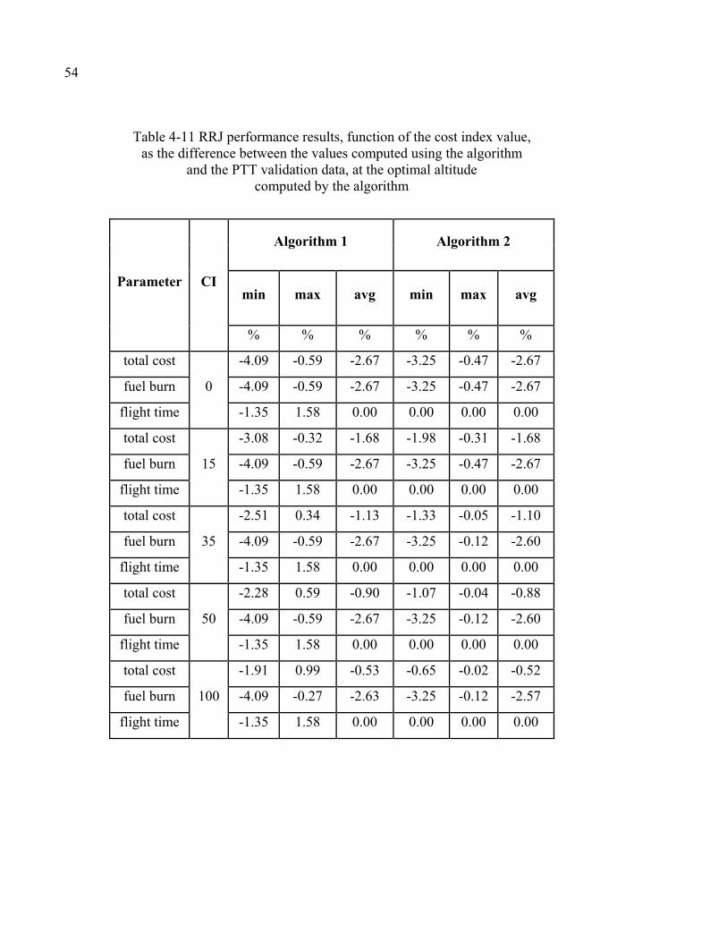
54

Table 4-11 RRJ performance results, function of the cost index value, as the difference between the values computed using the algorithm

and the PTT validation data, at the optimal altitude computed by the algorithm

Parameter CI

Algorithm 1 Algorithm 2

min max avg min max avg

% % % % % %

total cost

0

-4.09 -0.59 -2.67 -3.25 -0.47 -2.67

fuel burn -4.09 -0.59 -2.67 -3.25 -0.47 -2.67

flight time -1.35 1.58 0.00 0.00 0.00 0.00

total cost

15

-3.08 -0.32 -1.68 -1.98 -0.31 -1.68

fuel burn -4.09 -0.59 -2.67 -3.25 -0.47 -2.67

flight time -1.35 1.58 0.00 0.00 0.00 0.00

total cost

35

-2.51 0.34 -1.13 -1.33 -0.05 -1.10

fuel burn -4.09 -0.59 -2.67 -3.25 -0.12 -2.60

flight time -1.35 1.58 0.00 0.00 0.00 0.00

total cost

50

-2.28 0.59 -0.90 -1.07 -0.04 -0.88

fuel burn -4.09 -0.59 -2.67 -3.25 -0.12 -2.60

flight time -1.35 1.58 0.00 0.00 0.00 0.00

total cost

100

-1.91 0.99 -0.53 -0.65 -0.02 -0.52

fuel burn -4.09 -0.27 -2.63 -3.25 -0.12 -2.57

flight time -1.35 1.58 0.00 0.00 0.00 0.00

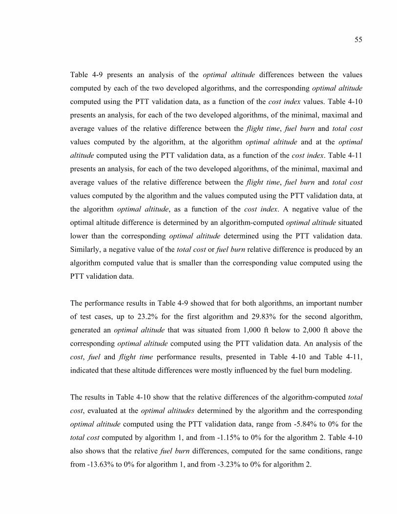
55

Table 4-9 presents an analysis of the optimal altitude differences between the values

computed by each of the two developed algorithms, and the corresponding optimal altitude

computed using the PTT validation data, as a function of the cost index values. Table 4-10

presents an analysis, for each of the two developed algorithms, of the minimal, maximal and

average values of the relative difference between the flight time, fuel burn and total cost

values computed by the algorithm, at the algorithm optimal altitude and at the optimal

altitude computed using the PTT validation data, as a function of the cost index. Table 4-11

presents an analysis, for each of the two developed algorithms, of the minimal, maximal and

average values of the relative difference between the flight time, fuel burn and total cost

values computed by the algorithm and the values computed using the PTT validation data, at

the algorithm optimal altitude, as a function of the cost index. A negative value of the

optimal altitude difference is determined by an algorithm-computed optimal altitude situated

lower than the corresponding optimal altitude determined using the PTT validation data.

Similarly, a negative value of the total cost or fuel burn relative difference is produced by an

algorithm computed value that is smaller than the corresponding value computed using the

PTT validation data.

The performance results in Table 4-9 showed that for both algorithms, an important number

of test cases, up to 23.2% for the first algorithm and 29.83% for the second algorithm,

generated an optimal altitude that was situated from 1,000 ft below to 2,000 ft above the

corresponding optimal altitude computed using the PTT validation data. An analysis of the

cost, fuel and flight time performance results, presented in Table 4-10 and Table 4-11,

indicated that these altitude differences were mostly influenced by the fuel burn modeling.

The results in Table 4-10 show that the relative differences of the algorithm-computed total

cost, evaluated at the optimal altitudes determined by the algorithm and the corresponding

optimal altitude computed using the PTT validation data, range from -5.84% to 0% for the

total cost computed by algorithm 1, and from -1.15% to 0% for the algorithm 2. Table 4-10

also shows that the relative fuel burn differences, computed for the same conditions, range

from -13.63% to 0% for algorithm 1, and from -3.23% to 0% for algorithm 2.

56

One important note relative to the Algorithm 1 flight time differences presented in the Table

4-10, for cost index values of 0 and 15: it can be observed that the min, max and average

values are 0. Following a detailed investigation, it was determined that this is due to the fact

that both FMS and algorithm determined optimal altitudes were situated at or above 36000ft,

in stratosphere, where the value of the speed of sound is constant with the altitude variation.

Therefore the corresponding ground speed and segment flight time are constant with altitude

variation.

The results in Table 4-11 show that the relative differences between the algorithm-computed

total cost, and the total cost computed using the PTT validation data, evaluated at the optimal

altitude computed by the algorithm, range from -4.09% to 0.99% for the total cost computed

by algorithm 1, and from -3.25% to -0.02% for the algorithm 2. Table 4-11 also shows that

the relative fuel burn differences, computed for the same conditions, range from

-4.09% to -0.27% for algorithm 1, and from -3.25% to -0.12% for algorithm 2. It can be

observed that the relative fuel burn difference corresponding to the algorithm 2 are always

negative. This means that the fuel burn value computed by the fuel burn algorithm, for an

altitude and flight time, is smaller than the fuel burn value computed by the PTT for the same

altitude and flight time. This is consistent with the fact that for the cg independent model, the

fuel burn rate variation with the fuel weight, and by consequence gw, is monotonous.

The algorithm execution time statistics, for the initialization, intermediary, and optimal

altitude module, respectively, are presented in Table 4-12, Table 4-13 and Table 4-14, below.

Table 4-12 RRJ Initialization module execution time statistics

Algorithm 1 Algorithm 2

min

time

max

time

average

time

min

time

max

time

average

time

s s s s s s

0.00008 0.0001 0.00009 0.00008 0.0014 0.00009

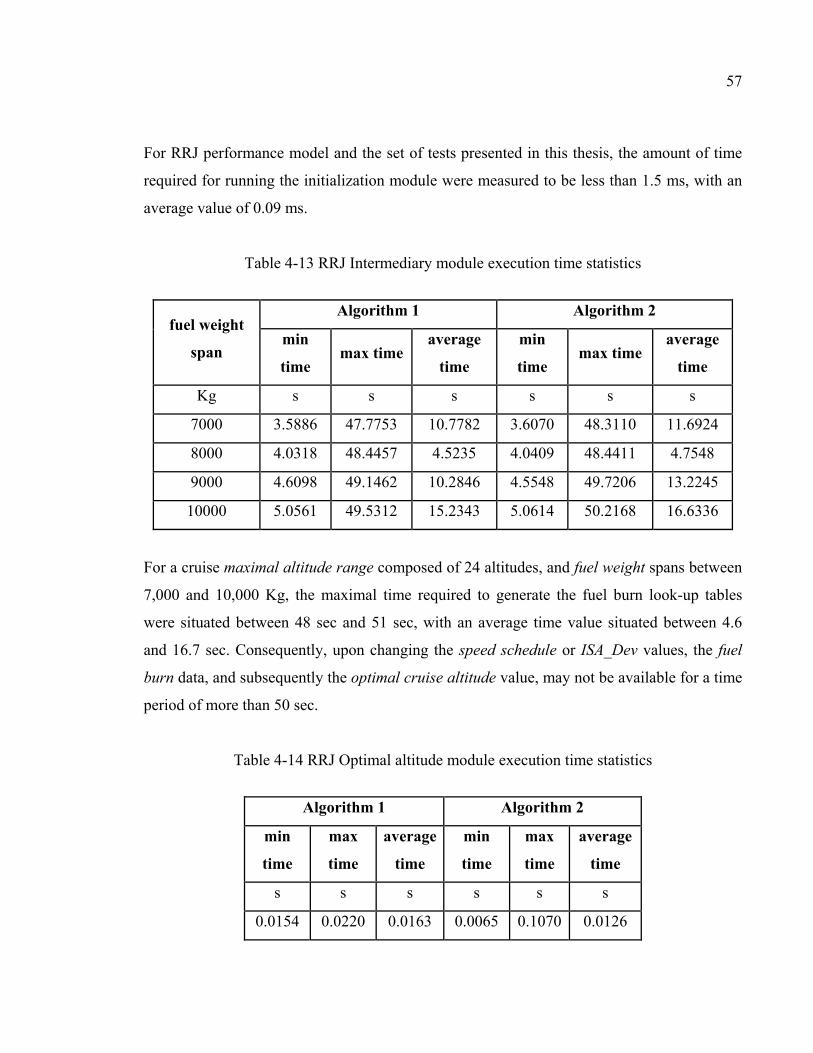
57

For RRJ performance model and the set of tests presented in this thesis, the amount of time

required for running the initialization module were measured to be less than 1.5 ms, with an

average value of 0.09 ms.

Table 4-13 RRJ Intermediary module execution time statistics

fuel weight

span

Algorithm 1 Algorithm 2

min

time max time

average

time

min

time max time

average

time

Kg s s s s s s

7000 3.5886 47.7753 10.7782 3.6070 48.3110 11.6924

8000 4.0318 48.4457 4.5235 4.0409 48.4411 4.7548

9000 4.6098 49.1462 10.2846 4.5548 49.7206 13.2245

10000 5.0561 49.5312 15.2343 5.0614 50.2168 16.6336

For a cruise maximal altitude range composed of 24 altitudes, and fuel weight spans between

7,000 and 10,000 Kg, the maximal time required to generate the fuel burn look-up tables

were situated between 48 sec and 51 sec, with an average time value situated between 4.6

and 16.7 sec. Consequently, upon changing the speed schedule or ISA_Dev values, the fuel

burn data, and subsequently the optimal cruise altitude value, may not be available for a time

period of more than 50 sec.

Table 4-14 RRJ Optimal altitude module execution time statistics

Algorithm 1 Algorithm 2

min

time

max

time

average

time

min

time

max

time

average

time

s s s s s s

0.0154 0.0220 0.0163 0.0065 0.1070 0.0126

58

The optimal altitude module time statistics, presented in Table 4-14, show that for still air

conditions, and a maximal cruise altitude range of 24 altitudes, the execution time were

situated between 15.4ms and 22ms, with an average value of 16.3ms.

59

4.3 The test results for Lockheed L1011

A number of 27 still air test configurations were considered, as described by the Table 4-15

below. They correspond to a cruise distance of 399.59 Nm. These configurations were

chosen to cover the aircraft’s range of IAS and Mach index speeds, zfgw, and fuel values. As

mentioned before, the objective of the validation was to compare the algorithm fuel burn

predictions with those computed by the PTT and the Flightsim.

The fuel burn difference values are presented as percentage of the fuel burn value extracted

from the Flightsim recorded data. A positive value represents an algorithm / PTT predicted

value that is larger than that corresponding to the Flightsim.

It can be observed that for all test cases the fuel burn differences between the algorithm and

Flightsim values ranged from 1.89% to 4.52%, whereas the difference between the PTT and

Flightsim values ranged from -1.34% to 6.59 % of the corresponding Flightsim value.

Considering the fact that the Flightsim computes the fuel burn in real time, its fuel burn value

should provide the closest approximation of the integral of the fuel burn rate, and is

considered the most accurate. By consequence, a negative value of the relative difference

between the PTT and Flightsim computed fuel burn corresponds to a PTT value that is lower

than the value of the integral of the fuel burn rate. However, the L1011 model is not cg-

dependent and its fbr variation with the gw is monotonous. Therefore, a PTT fuel burn value

that is lower that the Flightsim’ suggests that the algorithm that considers a constant fuel

burn rate on each cruise sub-segment may predict fuel burn values that are smaller than the

actual ones. More, for the majority of cases for which the PTT fuel burn is larger than the one

computed by the Flightsim, the value corresponding to the new proposed fuel burn algorithm

is closer to that of the Flightsim than the PTT value, therefore more accurate.

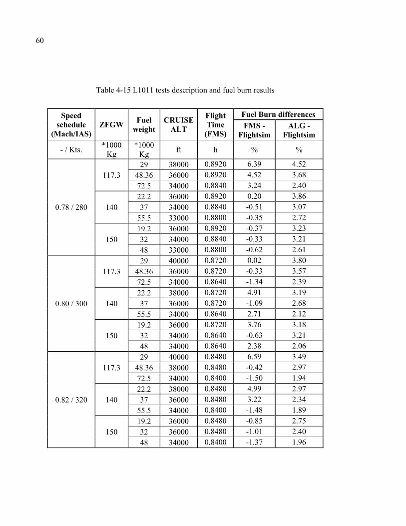
60

Table 4-15 L1011 tests description and fuel burn results

Speed schedule

(Mach/IAS) ZFGW

Fuel weight

CRUISE ALT

Flight Time

(FMS)

Fuel Burn differences

FMS - Flightsim

ALG - Flightsim

- / Kts. *1000

Kg *1000

Kg ft h % %

0.78 / 280

117.3 29 38000 0.8920 6.39 4.52

48.36 36000 0.8920 4.52 3.68

72.5 34000 0.8840 3.24 2.40

140 22.2 36000 0.8920 0.20 3.86

37 34000 0.8840 -0.51 3.07

55.5 33000 0.8800 -0.35 2.72

150 19.2 36000 0.8920 -0.37 3.23

32 34000 0.8840 -0.33 3.21

48 33000 0.8800 -0.62 2.61

0.80 / 300

117.3 29 40000 0.8720 0.02 3.80

48.36 36000 0.8720 -0.33 3.57

72.5 34000 0.8640 -1.34 2.39

140 22.2 38000 0.8720 4.91 3.19

37 36000 0.8720 -1.09 2.68

55.5 34000 0.8640 2.71 2.12

150 19.2 36000 0.8720 3.76 3.18

32 34000 0.8640 -0.63 3.21

48 34000 0.8640 2.38 2.06

0.82 / 320

117.3 29 40000 0.8480 6.59 3.49

48.36 38000 0.8480 -0.42 2.97

72.5 34000 0.8400 -1.50 1.94

140 22.2 38000 0.8480 4.99 2.97

37 36000 0.8480 3.22 2.34

55.5 34000 0.8400 -1.48 1.89

150 19.2 36000 0.8480 -0.85 2.75

32 36000 0.8480 -1.01 2.40

48 34000 0.8400 -1.37 1.96

CONCLUSIONS

The algorithm described in this thesis was implemented for a number of three aircraft

models, Airbus A310 which is cg dependent, Locheed L1011, and Sukhoi RRJ, which are not

cg dependent.

For the A310 and RRJ aircraft models, two versions of the algorithm were used for

validation, the original version of the algorithm proposed in this thesis - that performs all the

computations required to determine the optimal altitude, and a modified version - that uses

the cruise altitude range and corresponding flight times, computed by the PTT. The modified

version allowed for a better analyze of the differences between the fuel burn model proposed

in this thesis and that used by the PTT. The test scenarios investigated algorithm

performances, in still-air conditions, for an optimization distance of 500 Nm and five cost

index values (0, 15, 35, 50 and 100). This approach is consistent with the fact that the wind

conditions’ influence on the fuel burn and total cost are produced through the changes

induced in the value of the cruise segment’s flight time only. Therefore, the still air scenarios

allow for a good and accurate characterization of the fuel burn and optimal altitude

algorithms’ performances.

The test results showed that, depending on the cost index value, for up to 83% of A310 and

76% of RRJ test cases the optimal altitude computed by the algorithm was identical to that

computed using the PTT validation data. Also, for up to 23% of the test cases the optimal

altitudes were situated in a range of 2,000 ft from the values computed using the PTT

validation data. It is interesting to note that for the algorithm version that uses the PTT

computed flight times and A310 model, depending on the cost index value, the percentage

corresponding to identical values of optimal altitude rose up to 90%, while the percentage

corresponding to optimal altitude differences also rose up to 30%. For the RRJ model the

percentages remained virtually unchanged.

62

The test results for the A310 model, for the algorithm version that uses the PTT computed

flight times, also showed that for identical altitudes and flight times, the values of the fuel

burn computed by the algorithm were smaller for some test cases, and larger for other test

cases, than the values computed by the PTT. This is consistent with the fact that the cg

variation with the fuel weight, and by consequence gw, is not monotonous. Therefore, the fuel

burn rate computed by the algorithm may decrease on certain gross weight domains and

increase on others. Also, the results of the L1011 tests performed on the

Algorithm/PTT/Flightsim 9.1 platform indicated that the fuel burns predicted by the

algorithm were closer to the values extracted from the Flightsim recordings, which are

considered a close approximation of the fuel burn rate integral, than the values determined by

the PTT. This suggests that the fuel burn model implemented by the algorithm is better than

the model assuming constant fuel burn rates.

The analysis of the execution times of each of the main modules implementing the optimal

cruise altitude algorithm suggests that the algorithm can successfully observe the

requirements imposed by a real-time environment. The execution times for the initialization

module are very small compared with the time between the FMS configuration and aircraft

take-off, which is usually in the range of 15 to 30 minutes.

The intermediary module execution times were found to reach up to 150 sec for the cg-

dependent, and 51 sec for the cg-independent model. The delays caused by the fuel burn

look-up tables generation, upon a change of speed schedule or ISA_Dev values, are not

frequent and could be regarded as an algorithm limitation. A table generation and an update

policy adapted to the aircraft’s performances and selected optimization distance, in

conjunction with an appropriate minimal cruise altitude selection, could provide an important

reduction of the fuel burn look-up tables generation time.

The maximum response time of the optimal altitude module was determined to be of 103 ms.

Considering that the optimal cruise altitude value is computed or updated at time intervals of

63

no less than one minute, similar to other FMS data, we can conclude that the optimal altitude

module can successfully meet the optimal altitude computation and update time constraints.

In conclusion, the fuel burn algorithm presented in this thesis provides two important

features: Firstly, the value of the fuel burn considers the continuous variation of the fuel burn

rate with time, due to the variation of the fuel weight, thus it’s more accurate than that

considering constant fuel burn rates on sub-segments of 50 Nm. Secondly, it would no longer

require the decomposition of a cruise segment in smaller sub-segments, thus reducing the

volume of computations. This, in turn, opens the possibility for computing fuel burn values

for cruise flights spanning multiple segments, at once, using the corresponding total flight

time.

RECOMMENDATIONS

The analysis of the results presented in this thesis identified a number of directions, and

tasks, that could contribute to extending the characterization of algorithm’s performances,

and/or augment its capabilities.

The first recommendation addresses the generation of the FMS validation data, as it was the

principal factor limiting the number of test scenarios, and aircraft models, covered in this

thesis. It refers to identifying, or implementing a method that automates the process of

generation, and collection, of CMA 9000 FMS validation data, in collaboration with CMC

Electronics - Esterline. Subsequently, extending the number of test scenarios, both for still air

and constant wind conditions, would allow a more detailed characterization of the

algorithm’s performances and its advantages.

Other work may also include optimal cruise altitude algorithm improvement, with the

implementation of variable wind (wind blending) scenarios processing capabilities, and the

consideration of the costs, and fuel burns, associated with the climbs and descents imposed

by the cruise altitude change.

The optimal cruise altitude algorithm can be easily adapted for scenarios where the

optimization distance corresponds to a series of consecutive, independent, segments flown at

the same speed schedule and ISA_Dev values.

Finally, we propose the implementation of the fuel burn computation algorithm, presented in

this thesis, for all cruise, constant speed, level flight computations performed by the FMS.

LIST OF BIBLIOGRAPHIC REFERENCES

[1] Liden, S., 1994. “The evolution of Flight Management Systems”, Digital Avionics Systems Conference, 1994. 13th DASC., AIAA/IEEE, vol., no., pp.157-169, 30 Oct-3 Nov 1994. Online. <http://ieeexplore.ieee.org/stamp/stamp.jsp?tp=&arnumber=369487&isnumber=8448>. Retrieved on April 13, 2011

[2] Herndon, A.A.; Cramer, M.; Nicholson, T., 2009. "Analysis of advanced flight management systems (FMS), flight management computer (FMC) field observations, trials; lateral and vertical path integration" Digital Avionics Systems Conference, 2009. DASC '09. IEEE/AIAA 28th , vol., no., pp.1.C.2-1-1.C.2-16, 23-29 Oct. 2009. Online. <http://ieeexplore.ieee.org/stamp/stamp.jsp?tp=&arnumber=5347572&isnumber=5347412>. Retrieved on April 10, 2011

[3] Liden, S., 1992. "Optimum cruise profiles in the presence of winds," Digital Avionics Systems Conference, 1992. Proceedings., IEEE/AIAA 11th , vol., no., pp.254-261, 5-8 Oct 1992. Online. <http://ieeexplore.ieee.org/stamp/stamp.jsp?tp=&arnumber=282147&isnumber=6983>. Retrieved on May 7, 2010

[4] Liden, S., 1992. "Optimum 4D guidance for long flights," Digital Avionics Systems Conference, 1992. Proceedings., IEEE/AIAA 11th , vol., no., pp.262-267, 5-8 Oct 1992. Online. <http://ieeexplore.ieee.org/stamp/stamp.jsp?tp=&arnumber=282146&isnumber=6983http://ieeexplore.ieee.org/stamp/stamp.jsp?tp=&arnumber=282146&isnumber=6983>. Retrieved on May 22, 2010

[5] Liden, S., 1985. "Practical Considerations in Optimal Flight Management Computations," American Control Conference, 1985 , vol., no., pp.675-681, 19-21 June 1985. Online. <http://ieeexplore.ieee.org/stamp/stamp.jsp?tp=&arnumber=4788700&isnumber=4788561>. Retrieved on May 22, 2010

[6] Shufan Wu; Yongzhang Shen; , 1993. "Studies on the flight performance optimization of commercial aircrafts," TENCON '93. Proceedings. Computer, Communication, Control and Power Engineering.1993 IEEE Region 10 Conference on , vol., no.0, pp.139-145 vol.4, 19-21 Oct 1993. Online. <http://ieeexplore.ieee.org/stamp/stamp.jsp?tp=&arnumber=320453&isnumber=7692>. Retrieved on April 10, 2011

[7] Asselin, M., 1997, “AIAA Education Series: An Introduction to Aircraft Performance”, Reston, Virginia, USA: American Institute of Aeronautics and Astronautics, Inc.,339 p.

68

[8] Botez, R., 2006, GPA-745: Introduction à l’avionique: notes de cours GPA-745. Bachelor and Master’s engineering programs. Montreal: Ecole de Technologie Superieure, multiple pagination, 394 p.

[9] Botez, R., 2006, GPA-745: Introduction à l’avionique: notes de laboratoire GPA-745. Bachelor and Master’s engineering programs. Montreal: Ecole de Technologie Superieure, multiple pagination, 99 p.

[10] Federal Aviation Administration, 2007, "Aircraft Weight and Balance Handbook", Online. 97p. <http://www.faa.gov/library/manuals/aircraft/media/FAA-H-8083-1A.pdf>. Retrieved on November 10, 2010

[11] Butcher, J. C., 1987, “The numerical analysis of ordinary differential equations: Runge-Kutta and general linear methods”, New York, USA: Wiley-Interscience, 512 pages.