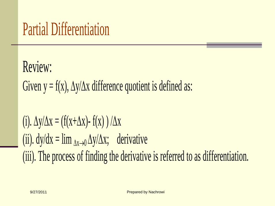
9/27/2011 Prepared by Nachrowi

Partial Differentiation Review: Given y = f(x), Δy/Δx difference quotient is defined as: (i). Δy/Δx = (f(x+Δx)- f(x) ) /Δx (ii). dy/dx = lim Δx→0 Δy/Δx; derivative (iii). The process of finding the derivative is referred to as differentiation.

9/27/2011 Prepared by Nachrowi

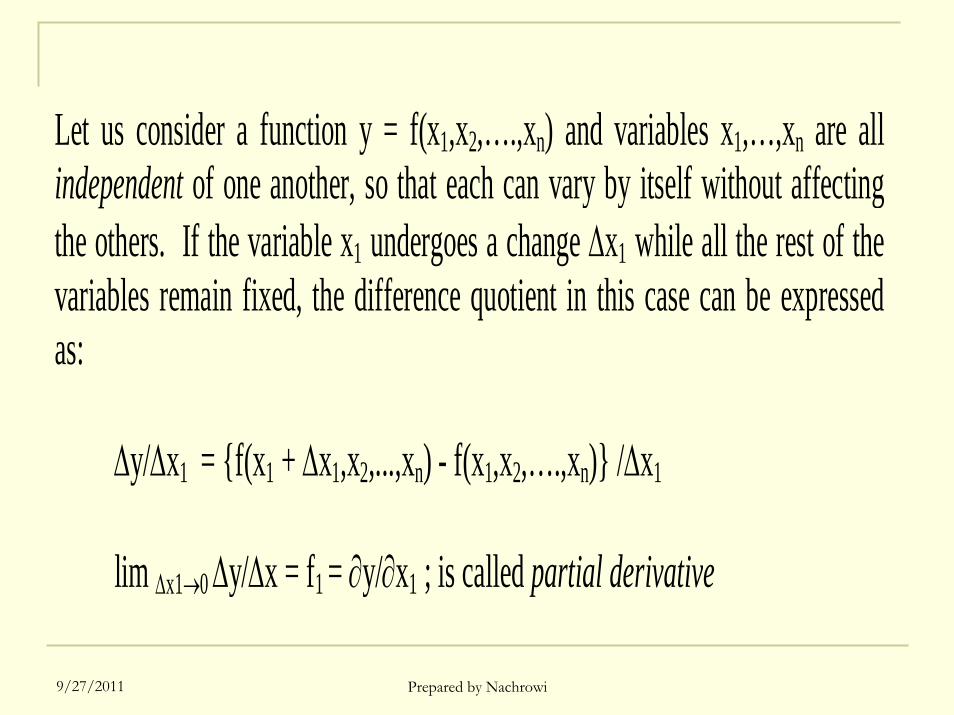
Let us consider a function y = f(x1,x2,….,xn) and variables x1,…,xn are allindependent of one another, so that each can vary by itself without affectingthe others. If the variable x1 undergoes a change Δx1 while all the rest of thevariables remain fixed, the difference quotient in this case can be expressedas: Δy/Δx1 = {f(x1 + Δx1,x2,...,xn) - f(x1,x2,….,xn)} /Δx1

lim Δx1→0 Δy/Δx = f1 = ∂y/∂x1 ; is called partial derivative

9/27/2011 Prepared by Nachrowi

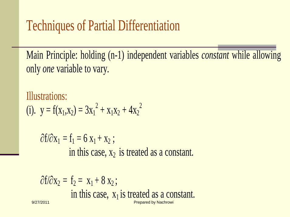
Techniques of Partial Differentiation Main Principle: holding (n-1) independent variables constant while allowing only one variable to vary. Illustrations: (i). y = f(x1,x2) = 3x1

2 + x1x2 + 4x22

∂f/∂x1 = f1 = 6 x1 + x2 ; in this case, x2 is treated as a constant. ∂f/∂x2 = f2 = x1 + 8 x2 ; in this case, x1 is treated as a constant.

9/27/2011 Prepared by Nachrowi

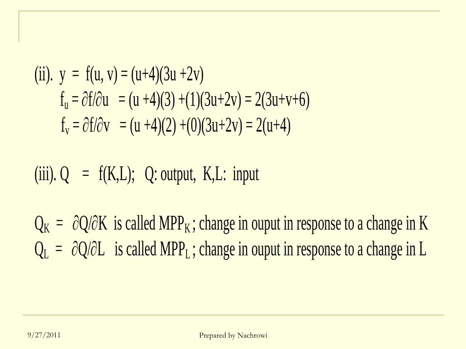
(ii). y = f(u, v) = (u+4)(3u +2v) fu = ∂f/∂u = (u +4)(3) +(1)(3u+2v) = 2(3u+v+6) fv = ∂f/∂v = (u +4)(2) +(0)(3u+2v) = 2(u+4) (iii). Q = f(K,L); Q: output, K,L: input QK = ∂Q/∂K is called MPPK ; change in ouput in response to a change in K QL = ∂Q/∂L is called MPPL ; change in ouput in response to a change in L

9/27/2011 Prepared by Nachrowi

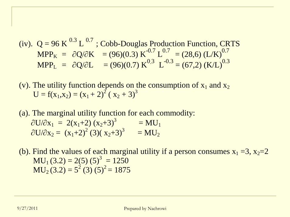
(iv). Q = 96 K 0.3 L 0.7 ; Cobb-Douglas Production Function, CRTS

MPPK = ∂Q/∂K = (96)(0.3) K-0.7 L0.7 = (28,6) (L/K)0.7 MPPL = ∂Q/∂L = (96)(0.7) K0.3 L-0.3 = (67,2) (K/L)0.3

(v). The utility function depends on the consumption of x1 and x2 U = f(x1,x2) = (x1 + 2)2 ( x2 + 3)3

(a). The marginal utility function for each commodity: ∂U/∂x1 = 2(x1+2) (x2+3)3 = MU1 ∂U/∂x2 = (x1+2)2 (3)( x2+3)3 = MU2

(b). Find the values of each marginal utility if a person consumes x1 =3, x2=2 MU1 (3.2) = 2(5) (5)3 = 1250 MU2 (3.2) = 52 (3) (5)2 = 1875

9/27/2011 Prepared by Nachrowi

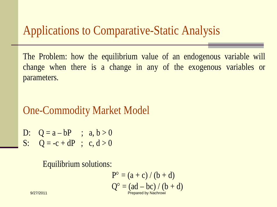
Applications to Comparative-Static Analysis The Problem: how the equilibrium value of an endogenous variable willchange when there is a change in any of the exogenous variables orparameters. One-Commodity Market Model D: Q = a – bP ; a, b > 0 S: Q = -c + dP ; c, d > 0 Equilibrium solutions: P° = (a + c) / (b + d) Q° = (ad – bc) / (b + d)

9/27/2011 Prepared by Nachrowi

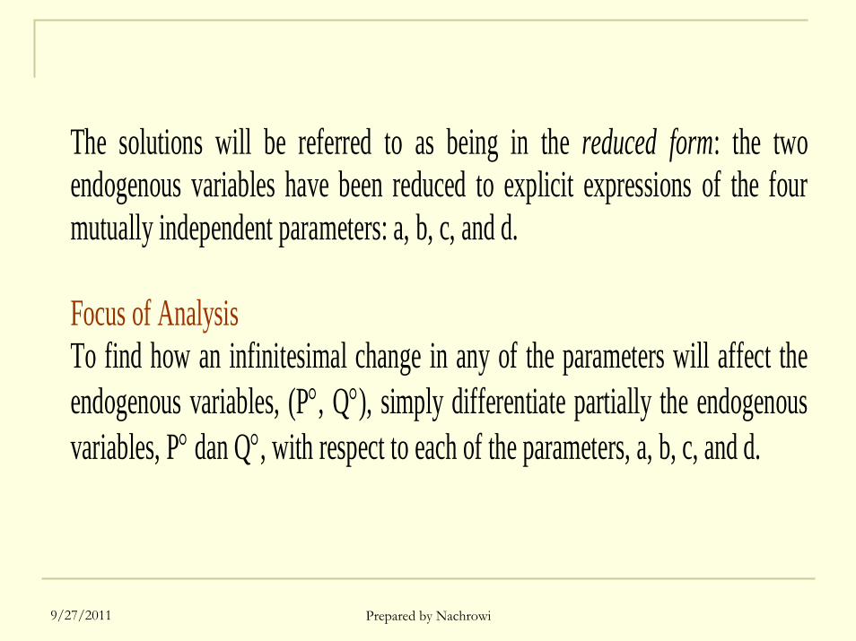
The solutions will be referred to as being in the reduced form: the two endogenous variables have been reduced to explicit expressions of the fourmutually independent parameters: a, b, c, and d. Focus of Analysis To find how an infinitesimal change in any of the parameters will affect theendogenous variables, (P°, Q°), simply differentiate partially the endogenousvariables, P° dan Q°, with respect to each of the parameters, a, b, c, and d.

9/27/2011 Prepared by Nachrowi

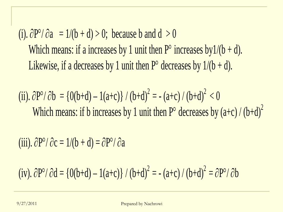
(i). ∂P°/ ∂a = 1/(b + d) > 0; because b and d > 0 Which means: if a increases by 1 unit then P° increases by1/(b + d). Likewise, if a decreases by 1 unit then P° decreases by 1/(b + d). (ii). ∂P°/ ∂b = {0(b+d) – 1(a+c)} / (b+d)2 = - (a+c) / (b+d)2 < 0 Which means: if b increases by 1 unit then P° decreases by (a+c) / (b+d)2 (iii). ∂P°/ ∂c = 1/(b + d) = ∂P°/ ∂a (iv). ∂P°/ ∂d = {0(b+d) – 1(a+c)} / (b+d)2 = - (a+c) / (b+d)2 = ∂P°/ ∂b

9/27/2011 Prepared by Nachrowi

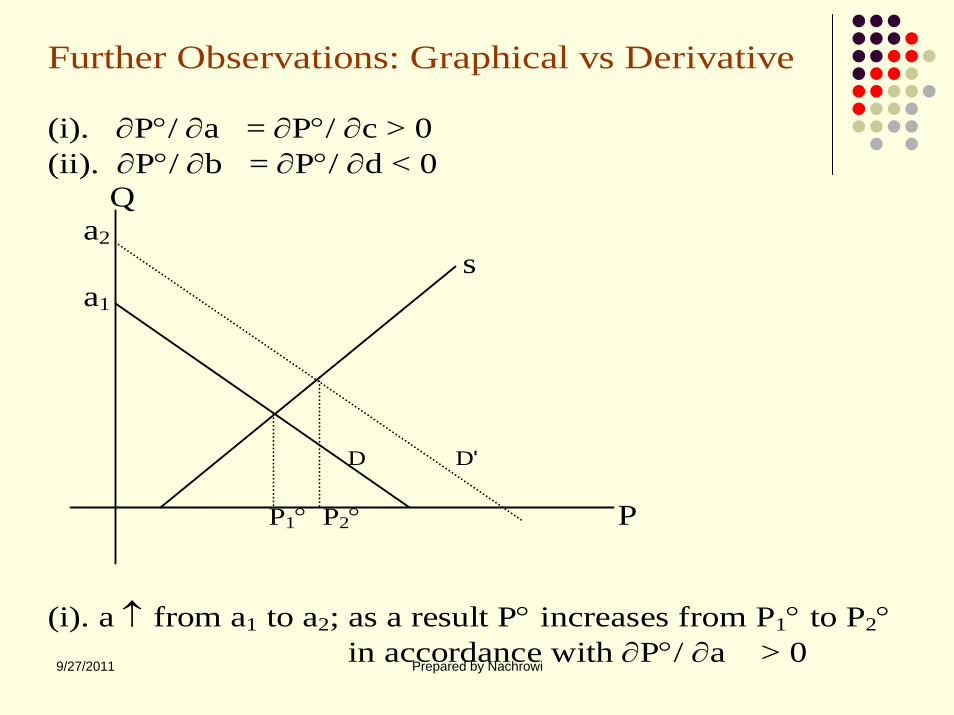
Further Observations: Graphical vs Derivative (i). ∂P°/ ∂a = ∂P°/ ∂c > 0 (ii). ∂P°/ ∂b = ∂P°/ ∂d < 0 Q a2 s a1 D D' P1° P2° P (i). a ↑ from a1 to a2; as a result P° increases from P1° to P2° in accordance with ∂P°/ ∂a > 0

9/27/2011 Prepared by Nachrowi

Q s s' D -c1 P1° P2° P -c2

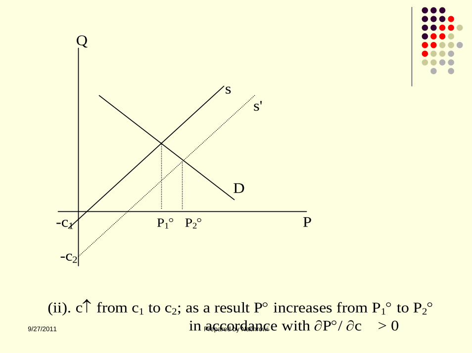
(ii). c↑ from c1 to c2; as a result P° increases from P1° to P2° in accordance with ∂P°/ ∂c > 0

9/27/2011 Prepared by Nachrowi

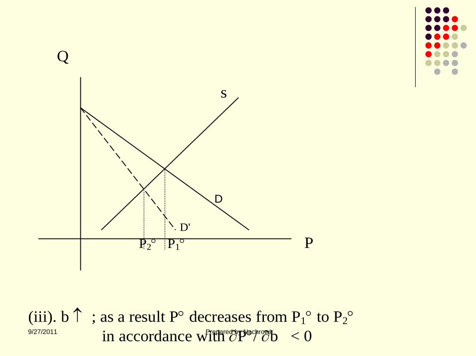
Q s D D' P2° P1° P (iii). b ↑ ; as a result P° decreases from P1° to P2° in accordance with ∂P°/ ∂b < 0

9/27/2011 Prepared by Nachrowi

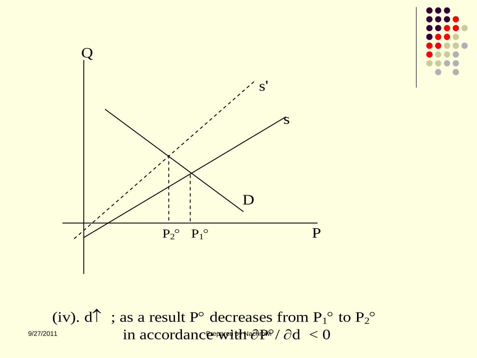
Q s' s D P2° P1° P (iv). d↑ ; as a result P° decreases from P1° to P2° in accordance with ∂P°/ ∂d < 0

9/27/2011 Prepared by Nachrowi

Comments:

• Since all the results seems to have beenobtainable graphically, then why should webother to learn differentiation at all?

9/27/2011 Prepared by Nachrowi

Advantages of Partial Derivative Analysis

1. Graphical technique is subject to a dimensional restriction, butdifferentiation is not. Even when the number of endogenous variablesand parameters is such that the equilibrium state cannot be showngraphically, we can nevertheless apply the differentiation techniques tothe problem.

2. The differentiation method can yield results that are on a higher level of

generality. The comparative-static conclusions in this model areapplicable to an infinite number of combinations of (linear) demandand supply functions. In contrast, the graphical approach deals onlywith some specific members of the family of demand and supply curve,strictly speaking, only to the specific functions depicted.

9/27/2011 Prepared by Nachrowi

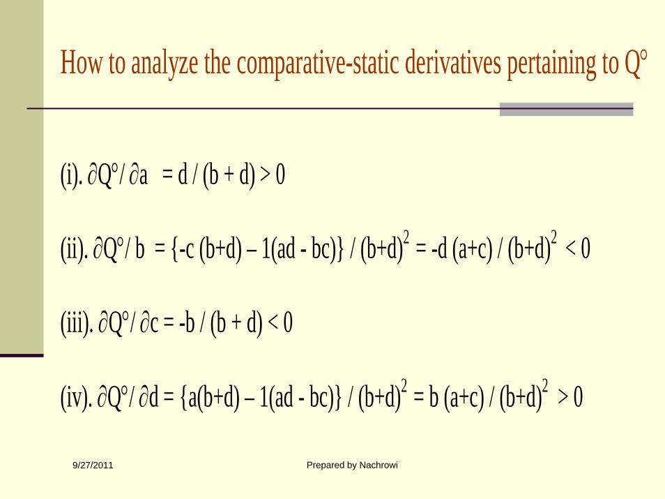
How to analyze the comparative-static derivatives pertaining to Q° (i). ∂Q°/ ∂a = d / (b + d) > 0 (ii). ∂Q°/ b = {-c (b+d) – 1(ad - bc)} / (b+d)2 = -d (a+c) / (b+d)2 < 0 (iii). ∂Q°/ ∂c = -b / (b + d) < 0 (iv). ∂Q°/ ∂d = {a(b+d) – 1(ad - bc)} / (b+d)2 = b (a+c) / (b+d)2 > 0

9/27/2011 Prepared by Nachrowi

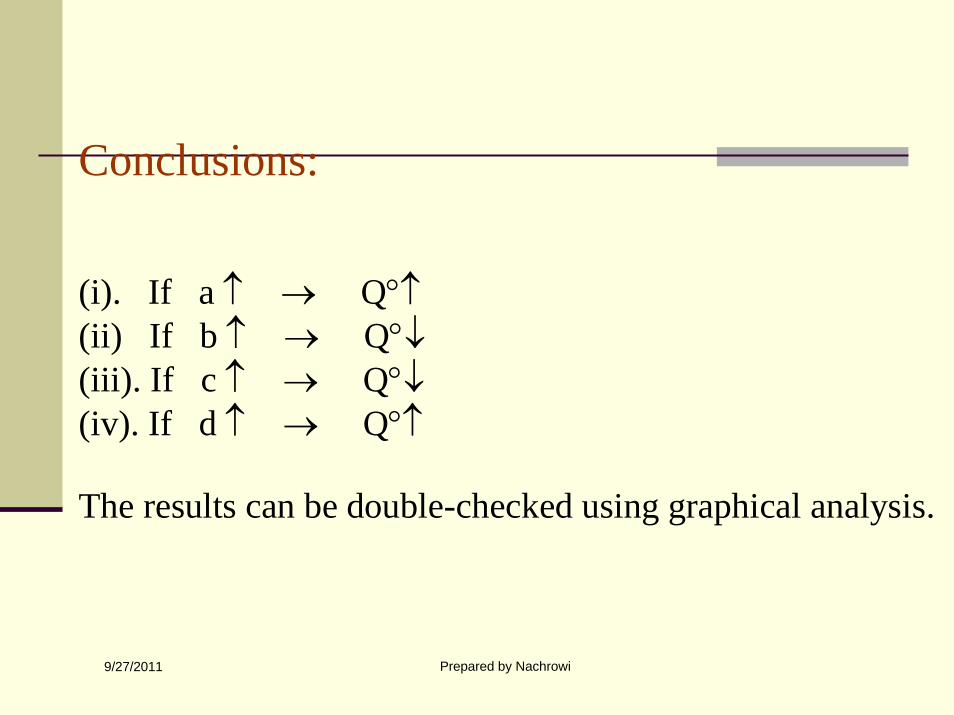
Conclusions: (i). If a ↑ → Q°↑ (ii) If b ↑ → Q°↓ (iii). If c ↑ → Q°↓ (iv). If d ↑ → Q°↑ The results can be double-checked using graphical analysis.

9/27/2011 Prepared by Nachrowi

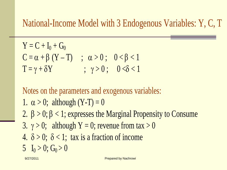
National-Income Model with 3 Endogenous Variables: Y, C, T Y = C + I0 + G0 C = α + β (Y – T) ; α > 0 ; 0 < β < 1 T = γ + δY ; γ > 0 ; 0 <δ < 1 Notes on the parameters and exogenous variables: 1. α > 0; although (Y-T) = 0 2. β > 0; β < 1; expresses the Marginal Propensity to Consume 3. γ > 0; although Y = 0; revenue from tax > 0 4. δ > 0; δ < 1; tax is a fraction of income 5 I0 > 0; G0 > 0

9/27/2011 Prepared by Nachrowi

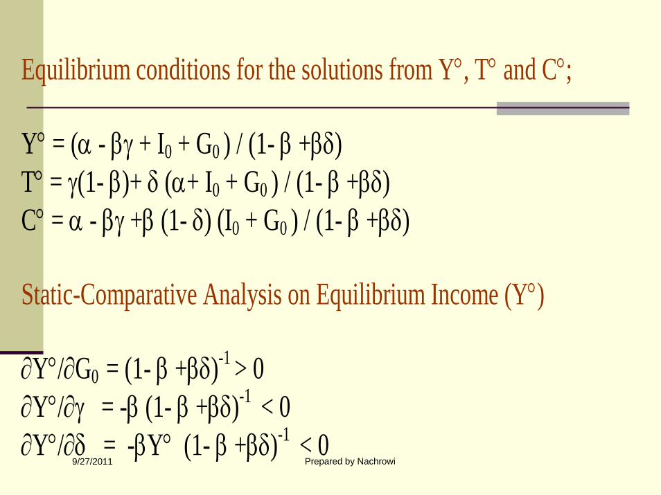
Equilibrium conditions for the solutions from Y°, T° and C°; Y° = (α - βγ + I0 + G0 ) / (1- β +βδ) T° = γ(1- β)+ δ (α+ I0 + G0 ) / (1- β +βδ) C° = α - βγ +β (1- δ) (I0 + G0 ) / (1- β +βδ) Static-Comparative Analysis on Equilibrium Income (Y°) ∂Y°/∂G0 = (1- β +βδ)-1 > 0 ∂Y°/∂γ = -β (1- β +βδ)-1 < 0 ∂Y°/∂δ = -βY° (1- β +βδ)-1 < 0

9/27/2011 Prepared by Nachrowi

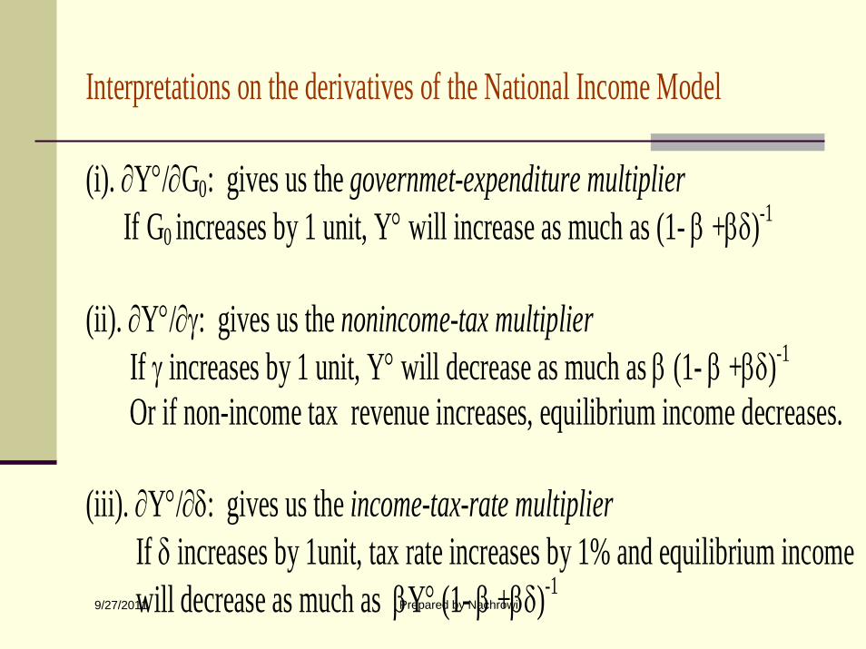
Interpretations on the derivatives of the National Income Model (i). ∂Y°/∂G0: gives us the governmet-expenditure multiplier If G0 increases by 1 unit, Y° will increase as much as (1- β +βδ)-1

(ii). ∂Y°/∂γ: gives us the nonincome-tax multiplier If γ increases by 1 unit, Y° will decrease as much as β (1- β +βδ)-1 Or if non-income tax revenue increases, equilibrium income decreases. (iii). ∂Y°/∂δ: gives us the income-tax-rate multiplier If δ increases by 1unit, tax rate increases by 1% and equilibrium income will decrease as much as βY° (1- β +βδ)-1

9/27/2011 Prepared by Nachrowi

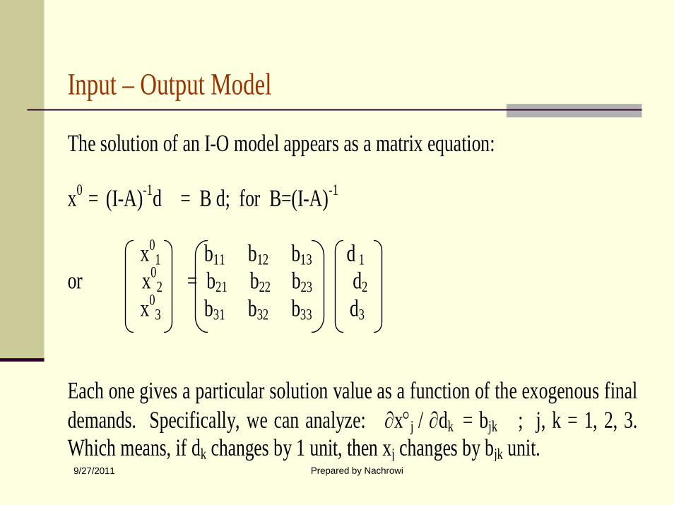
Input – Output Model The solution of an I-O model appears as a matrix equation: x0 = (I-A)-1d = B d; for B=(I-A)-1 x0

1 b11 b12 b13 d 1 or x0

2 = b21 b22 b23 d2 x0

3 b31 b32 b33 d3 Each one gives a particular solution value as a function of the exogenous finaldemands. Specifically, we can analyze: ∂x°j / ∂dk = bjk ; j, k = 1, 2, 3. Which means, if dk changes by 1 unit, then xj changes by bjk unit.

9/27/2011 Prepared by Nachrowi

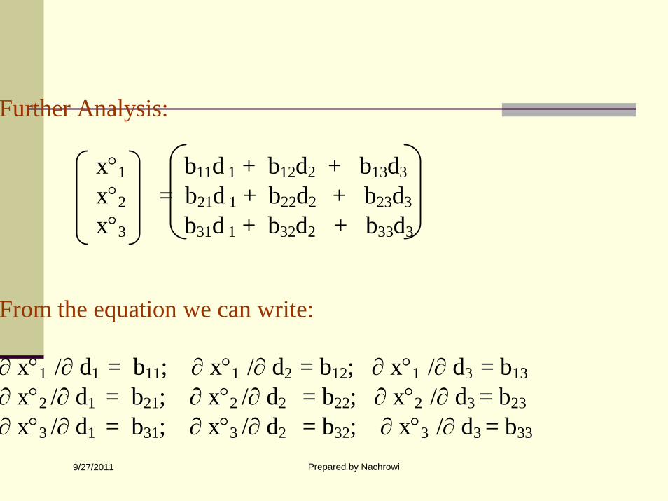
Further Analysis: x°1 b11d 1 + b12d2 + b13d3 x°2 = b21d 1 + b22d2 + b23d3 x°3 b31d 1 + b32d2 + b33d3 From the equation we can write: ∂ x°1 /∂ d1 = b11; ∂ x°1 /∂ d2 = b12; ∂ x°1 /∂ d3 = b13 ∂ x°2 /∂ d1 = b21; ∂ x°2 /∂ d2 = b22; ∂ x°2 /∂ d3 = b23 ∂ x°3 /∂ d1 = b31; ∂ x°3 /∂ d2 = b32; ∂ x°3 /∂ d3 = b33

9/27/2011 Prepared by Nachrowi

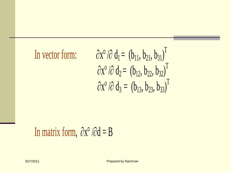
In vector form: ∂x° /∂ d1 = (b11, b21, b31)T

∂x° /∂ d2 = (b12, b22, b32)T

∂x° /∂ d3 = (b13, b23, b33)T

In matrix form, ∂x° /∂d = B

9/27/2011 Prepared by Nachrowi

Jacobian Determinants or Jacobian

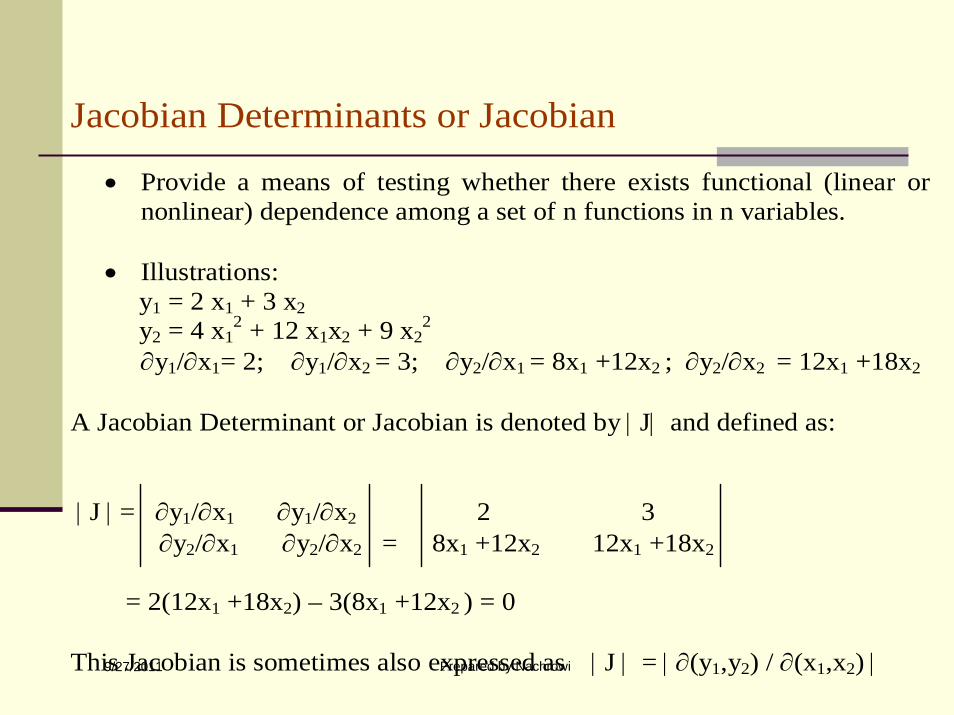
• Provide a means of testing whether there exists functional (linear ornonlinear) dependence among a set of n functions in n variables.

• Illustrations:

y1 = 2 x1 + 3 x2 y2 = 4 x1

2 + 12 x1x2 + 9 x22

∂y1/∂x1= 2; ∂y1/∂x2 = 3; ∂y2/∂x1 = 8x1 +12x2 ; ∂y2/∂x2 = 12x1 +18x2 A Jacobian Determinant or Jacobian is denoted by | J| and defined as: | J | = ∂y1/∂x1 ∂y1/∂x2 2 3 ∂y2/∂x1 ∂y2/∂x2 = 8x1 +12x2 12x1 +18x2 = 2(12x1 +18x2) – 3(8x1 +12x2 ) = 0 This Jacobian is sometimes also expressed as | J | = | ∂(y1,y2) / ∂(x1,x2) |

9/27/2011 Prepared by Nachrowi

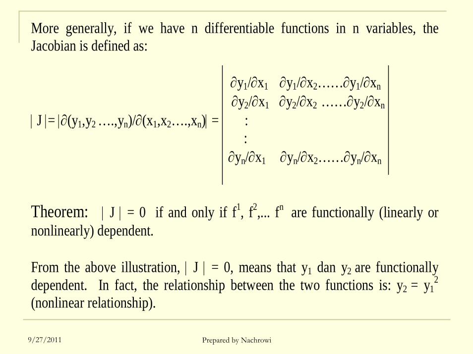
More generally, if we have n differentiable functions in n variables, theJacobian is defined as: ∂y1/∂x1 ∂y1/∂x2……∂y1/∂xn ∂y2/∂x1 ∂y2/∂x2 ……∂y2/∂xn | J |= |∂(y1,y2 ….,yn)/∂(x1,x2….,xn)| = : : ∂yn/∂x1 ∂yn/∂x2……∂yn/∂xn

Theorem: | J | = 0 if and only if f1, f2,... fn are functionally (linearly ornonlinearly) dependent. From the above illustration, | J | = 0, means that y1 dan y2 are functionallydependent. In fact, the relationship between the two functions is: y2 = y1

2

(nonlinear relationship).

9/27/2011 Prepared by Nachrowi

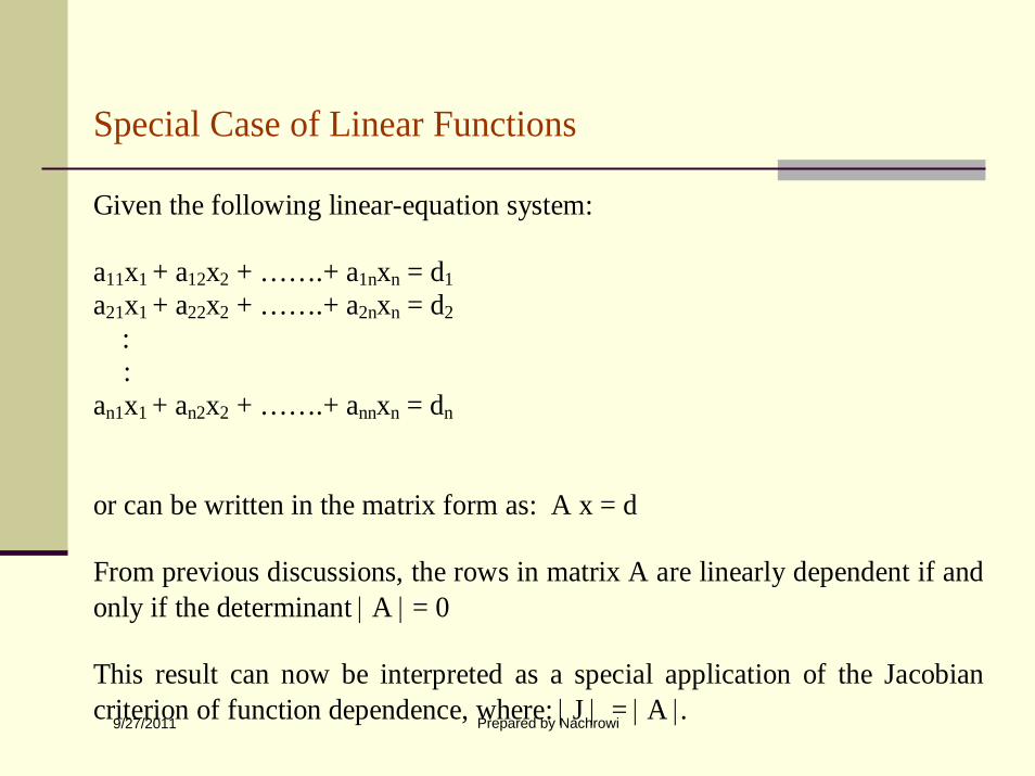
Special Case of Linear Functions Given the following linear-equation system: a11x1 + a12x2 + …….+ a1nxn = d1 a21x1 + a22x2 + …….+ a2nxn = d2 : : an1x1 + an2x2 + …….+ annxn = dn or can be written in the matrix form as: A x = d From previous discussions, the rows in matrix A are linearly dependent if andonly if the determinant | A | = 0 This result can now be interpreted as a special application of the Jacobiancriterion of function dependence, where: | J | = | A |.

9/27/20119/27/2011 Prepared by NachrowiPrepared by Nachrowi

The end of The end of the lessonthe lesson

Created by Nachrowi D. NachrowiCreated by Nachrowi D. Nachrowi