Week 1: Review

Tsun-Feng Chiang*

*School of Economics, Henan University, Kaifeng, China

March 1, 2014

1 / 25

Review Classical Assumption

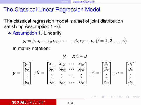
The Classical Linear Regression Model

The classical regression model is a set of joint distributionsatisfying Assumption 1 - 6:

Assumption 1. Linearity

yi = β1xi1 + β2xi2 + · · ·+ βK xiK + ui (i = 1,2, . . . ,n)

In matrix notation:

y = Xβ + u

y =

y1y2...

yn

, X =

x11 x12 · · · x1Kx21 x22 · · · x2K...

... . . . ...xn1 xn2 · · · xnK

, β =

β1β2...βK

, u =

u1u2...

un

2 / 25

Review Classical Assumption

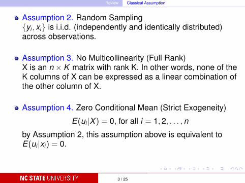
Assumption 2. Random Sampling{yi , xi} is i.i.d. (independently and identically distributed)across observations.

Assumption 3. No Multicollinearity (Full Rank)X is an n × K matrix with rank K. In other words, none of theK columns of X can be expressed as a linear combination ofthe other column of X.

Assumption 4. Zero Conditional Mean (Strict Exogeneity)

E(ui |X ) = 0, for all i = 1,2, . . . ,n

by Assumption 2, this assumption above is equivalent toE(ui |xi) = 0.

3 / 25

Review Classical Assumption

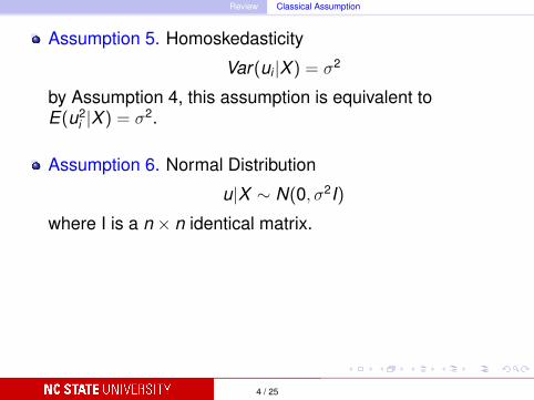
Assumption 5. Homoskedasticity

Var(ui |X ) = σ2

by Assumption 4, this assumption is equivalent toE(u2

i |X ) = σ2.

Assumption 6. Normal Distribution

u|X ∼ N(0, σ2I)

where I is a n × n identical matrix.

4 / 25

Review Ordinary Least Square

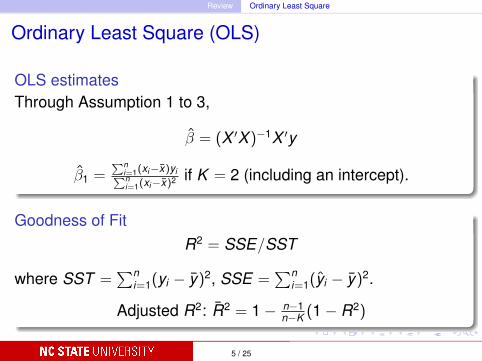
Ordinary Least Square (OLS)

OLS estimatesThrough Assumption 1 to 3,

β = (X ′X )−1X ′y

β1 =∑n

i=1(xi−x)yi∑ni=1(xi−x)2 if K = 2 (including an intercept).

Goodness of FitR2 = SSE/SST

where SST =∑n

i=1(yi − y)2, SSE =∑n

i=1(yi − y)2.

Adjusted R2: R2 = 1− n−1n−K (1− R2)

5 / 25

Review Ordinary Least Square

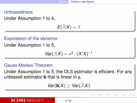
UnbiasednessUnder Assumption 1 to 4,

E(β|X ) = β

Expression of the varianceUnder Assumption 1 to 5,

Var(β|X ) = σ2 · (X ′X )−1

Gauss-Markov TheoremUnder Assumption 1 to 5, the OLS estimator is efficient. For anyunbiased estimator b that is linear in y,

Var(b|X ) ≥ Var(β|X )

6 / 25

Review Ordinary Least Square

BLUEBecause the regression model is linear, the estimators areunbiased and efficient (Gauss-Markov Theorem), the OLSestimator is called Best Linear Unbiased Estimator (BLUE).

7 / 25

Review Ordinary Least Square

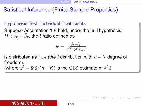
Satistical Inference (Finite-Sample Properties)

Hypothesis Test: Individual CoefficientsSuppose Assumption 1-6 hold, under the null hypothesisH0 : βk = βk , the t-ratio defined as

tk = βk−βk√s2·(X ′X)−1

kk

is distributed as tn−K (the t distribution with n − K degree offreedom).(where s2 = u′u/(n − K ) is the OLS estimate of σ2.)

8 / 25

Review Ordinary Least Square

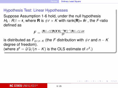
Hypothesis Test: Linear HypothessesSuppose Assumption 1-6 hold, under the null hypothesisH0 : Rβ = r, where R is #r × K with rank(R)= #r , the F -ratiodefined as

F = (Rβ−r)′[R(X′X)−1R′]−1(Rβ−r)/#rS2

is distributed as F#r ,n−K (the F distribution with #r and n − Kdegree of freedom).(where s2 = u′u/(n − K ) is the OLS estimate of σ2.)

9 / 25

Review Heteroskedasticity

Heteroskedasticity

Violation of Assumption 5Because Assumption 1 to 4 hold, the OLS estimators are stillunbiased. However, they are not efficient anymore.

Formal DetectionsBreusch-Pagan testWhite test

RemedyRobust Standard Error (OLS)Weighted Least Square (WLS)

10 / 25

Use R

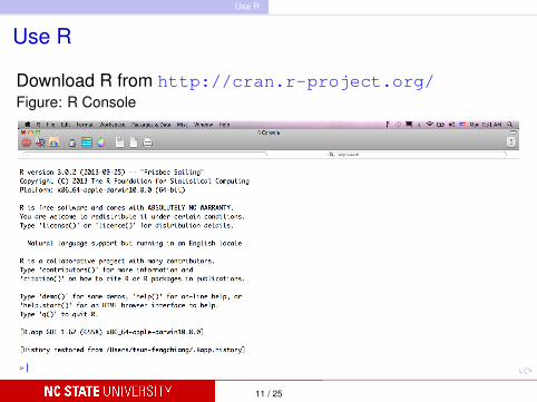
Use R

Download R from http://cran.r-project.org/Figure: R Console

11 / 25

Use R

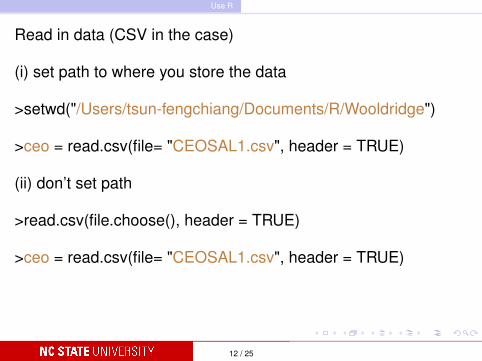
Read in data (CSV in the case)

(i) set path to where you store the data

>setwd("/Users/tsun-fengchiang/Documents/R/Wooldridge")

>ceo = read.csv(file= "CEOSAL1.csv", header = TRUE)

(ii) don’t set path

>read.csv(file.choose(), header = TRUE)

>ceo = read.csv(file= "CEOSAL1.csv", header = TRUE)

12 / 25

Use R

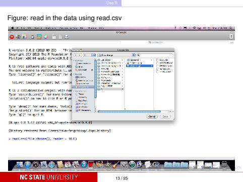
Figure: read in the data using read.csv

13 / 25

Use R

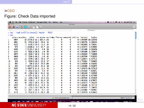
>ceoFigure: Check Data imported

14 / 25

Use R OLS

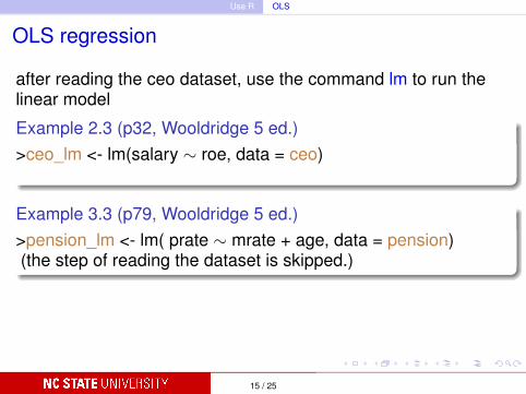
OLS regression

after reading the ceo dataset, use the command lm to run thelinear model

Example 2.3 (p32, Wooldridge 5 ed.)>ceo_lm <- lm(salary ∼ roe, data = ceo)

Example 3.3 (p79, Wooldridge 5 ed.)>pension_lm <- lm( prate ∼ mrate + age, data = pension)(the step of reading the dataset is skipped.)

15 / 25

Use R OLS

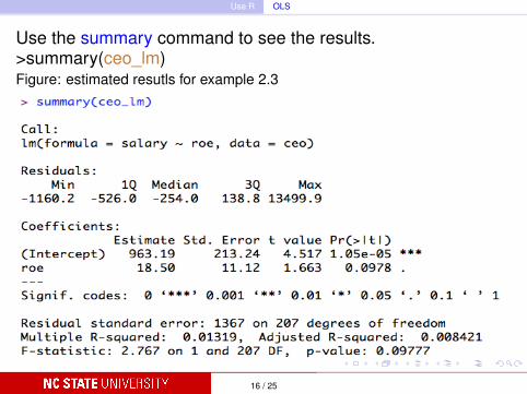
Use the summary command to see the results.>summary(ceo_lm)Figure: estimated resutls for example 2.3

16 / 25

Use R OLS

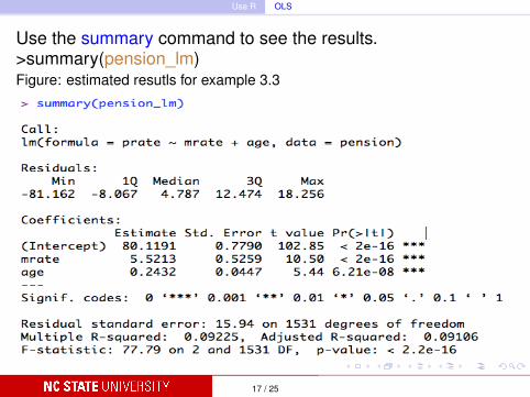
Use the summary command to see the results.>summary(pension_lm)Figure: estimated resutls for example 3.3

17 / 25

Use R OLS

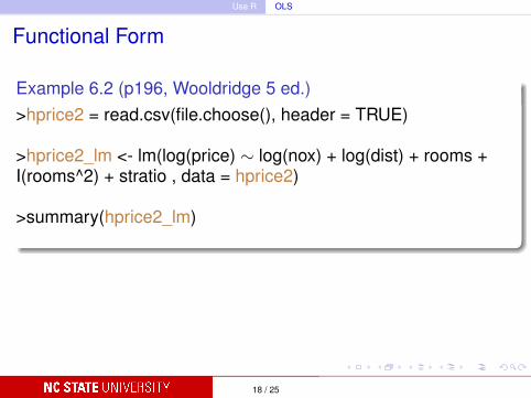
Functional Form

Example 6.2 (p196, Wooldridge 5 ed.)>hprice2 = read.csv(file.choose(), header = TRUE)

>hprice2_lm <- lm(log(price) ∼ log(nox) + log(dist) + rooms +I(rooms^2) + stratio , data = hprice2)

>summary(hprice2_lm)

18 / 25

Use R Heteroskedasticity

Heteroskedasticity

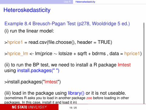
Example 8.4 Breusch-Pagan Test (p278, Wooldridge 5 ed.)(i) run the linear model:

>hprice1 = read.csv(file.choose(), header = TRUE)

>hprice_lm <- lm(price ∼ lotsize + sqrft + bdrms , data = hprice1)

(ii) to run the BP test, we need to install a R package lmtestusing install.packages(" ")

>install.packages("lmtest")

(iii) load in the package using library() or it is not useable.(sometimes R asks you to load in another package zoo before loading in otherpackages. In this case, install it and load it in)

19 / 25

Use R Heteroskedasticity

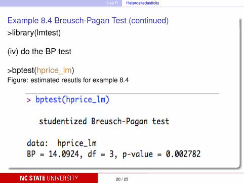
Example 8.4 Breusch-Pagan Test (continued)>library(lmtest)

(iv) do the BP test

>bptest(hprice_lm)Figure: estimated resutls for example 8.4

20 / 25

Use R Heteroskedasticity

Example 8.6 Robust Standard Error (p283-284, Wooldridge 5ed.)(i) run the linear model

>finance = read.csv(file.choose(), header = TRUE)

>finance_lm <- lm(nettfa ∼ inc + I((age-25)^2) + male + e401k ,data = finance)

>summary(finance_lm)

(ii) to run the robust standard error, we need to install a Rpackage sandwich using install.packages(" ")

>install.packages("sandwich")

21 / 25

Use R Heteroskedasticity

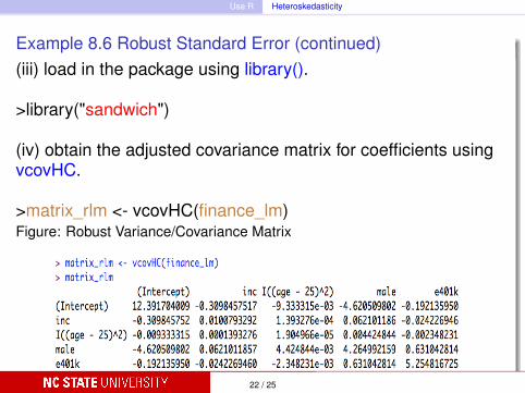
Example 8.6 Robust Standard Error (continued)(iii) load in the package using library().

>library("sandwich")

(iv) obtain the adjusted covariance matrix for coefficients usingvcovHC.

>matrix_rlm <- vcovHC(finance_lm)Figure: Robust Variance/Covariance Matrix

22 / 25

Use R Heteroskedasticity

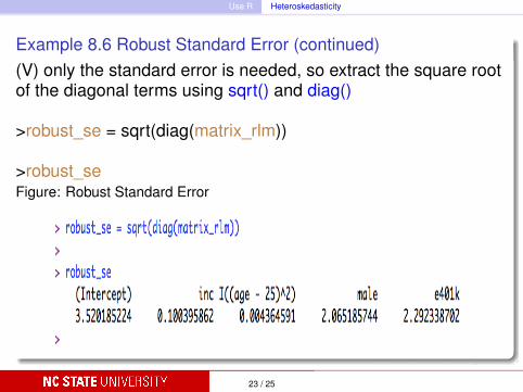
Example 8.6 Robust Standard Error (continued)(V) only the standard error is needed, so extract the square rootof the diagonal terms using sqrt() and diag()

>robust_se = sqrt(diag(matrix_rlm))

>robust_seFigure: Robust Standard Error

23 / 25

Use R Heteroskedasticity

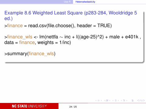
Example 8.6 Weighted Least Square (p283-284, Wooldridge 5ed.)>finance = read.csv(file.choose(), header = TRUE)

>finance_wls <- lm(nettfa ∼ inc + I((age-25)^2) + male + e401k ,data = finance, weights = 1/inc)

>summary(finance_wls)

24 / 25

Use R Heteroskedasticity

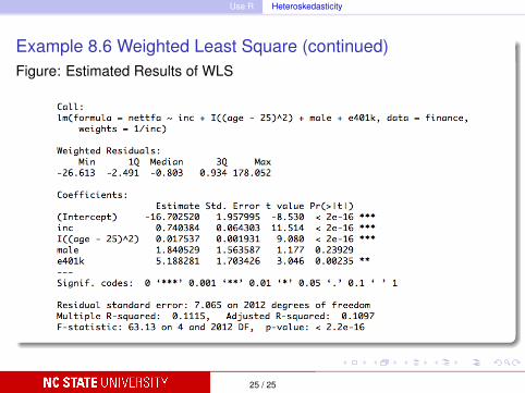
Example 8.6 Weighted Least Square (continued)Figure: Estimated Results of WLS

25 / 25