Chapter 8

Microcanonical ensemble

8.1 Definition

We consider an isolated system with N particles and energy E in a volume V . Bydefinition, such a system exchanges neither particles nor energy with the surroundings.

Uniform distribution of microstates. The assumption, that thermal equilibriumimplies that the distribution function ρ(q, p) of the system is a function of its energy,

ρ(q, p) = ρ(H(q, p)),d

dtρ(q, p) =

∂ρ

∂HE ≡ 0 ,

leads to to a constant ρ(q, p), which is manifestly consistent with the ergodic hypothesisand the postulate of a priori equal probabilities discussed in Sect. 7.5.

Energy shell. We consider a small but finite shell [E,E+Δ] close to the energy surface.The microcanonical ensemble is then defined by

ρ(q, p) =

1

Γ(E, V,N)E < H(q, p) < E +Δ

0 otherwise microcanonicalensemble

(8.1)

We defined in (8.1) with

Γ(E, V,N) =

� �

E<H(q,p)<E+Δ

d3Nq d3Np (8.2)

the volume occupied by the microcanonical ensemble.This is the volume of the shell bounded by the twoenergy surfaces with energies E and E +Δ

The dependence on the spatial volume V comes (8.2) from the limits of the integrationover dqi.

Infinitesimal shell. Let Φ(E, V ) be the total volume of phase space enclosed by theenergy surface E. We then have that

Γ(E) = Φ(E +Δ)− Φ(E) .

85

86 CHAPTER 8. MICROCANONICAL ENSEMBLE

Taking with Δ → 0 the limit of an infinitesimal shell thickness we obtain

Γ(E) =∂Φ(E)

∂EΔ ≡ Ω(E)Δ, Δ � E . (8.3)

Density of states. The quantity Ω(E),

Ω(E) =∂Φ(E)

∂E=

�d3Nq

�d3Np δ(E −H(q, p)) , (8.4)

is the density of states at energy E. The distribution of microstates ρ is therefore givenin terms of Ω(E), as

ρ(q, p) =

1

Ω(E)ΔE < H(q, p) < E +Δ

0 otherwise

Note that the formal divergence of ρ(q, p) with 1/Δ. We will discuss in Sect. 8.2.4 thatthe actual value of Δ is not of importance.

8.2 Entropy

The expectation value of a classical observable O(q, p) can be obtained by averaging overthe probability density ρ(q, p) of the microcanonical ensemble,

�O� =

�d3Nq d3Np ρ(q, p) O(q, p) =

1

Γ(E, V,N)

� �

E<H(q,p)<E+Δ

d3Nq d3Np O(q, p)

The entropy can however not been be obtained as an average of a classical observable. Itis instead a function of the overall number of available states.

POSTULATE The entropy is, according to Boltzmann, proportional to thelogarithm of the number of available states, as measured bythe phase space volume Γ:

S = kB ln

�Γ(E, V,N)

Γ0(N)

�(8.5)

We will now discuss the ramification of this definition.

Normalization factor. The normalization constant Γ0(N) introduced in (8.5) has twofunctionalities.

– Γ0(N) cancels the dimensions of Γ(E, V,N). The argument of the logarithm isconsequently dimensionless.

8.2. ENTROPY 87

– The number of particles N is one of the fundamental thermodynamic variables. Thefunctional dependence of Γ0(N) on N is hence important.

Incompleteness of classical statistics. It is not possible to determine Γ0(N) correctlywithin classical statistics. We will derive lateron that Γ0(N) takes the value

Γ0(N) = h3NN ! , (8.6)

in quantum statistics, where h = 6.63 · 10−34 m2kg/s is the Planck constant. We considerthis value also for classical statistics.

– The factor h3N defines the reference measure in phase space which has the dimen-sions [q]3N [p]3N . Note that [h] = m (kgm/s) = [q][p].

– N ! is the counting factor for states obtained by permuting particles.

The factor N ! arises from the fact that particles are indistin-guishable.Even though one may be in a temperature and density rangewhere the motion of molecules can be treated to a very goodapproximation by classical mechanics, one cannot go so far asto disregard the essential indistinguishability of the molecules;one cannot observe and label individual atomic particles asthough they were macroscopic billiard balls.

We will discuss in Sect. 8.2.1 the Gibbs paradox, which arises when on regards the con-stituent particles as distinguishable. In this case there would be no factor N ! in Γ0(N).

The entropy as an expectation value. We rewrite the definition (8.5) of the entropyas

S = −kB ln

�Γ0(N)

Γ(E, V,N)

�= −kB

� �d3Nq d3Np ρ(q, p) ln

�Γ0(N)ρ(q, p)

�, (8.7)

where we have used that ρ(q, p) = 1/Γ(E, V,N) within the energy shell and that� �

d3Nq d3Np ρ(q, p) =

�

E<H<E+Δ

d3Nq d3Np/Γ(E, V,N) = 1 .

We hence have

S = −kB�ln[Γ0(N)ρ(q, p)]

�.

The entropy coincides hence with Shannon’s information-theoretical definition of the en-tropy, apart from the factors kB and Γ0(N), as discussed in Sect. 5.5.3.

Thermodynamic consistency. Since we have introduced the entropy definition in anad-hoc way, we need to convince ourselves that it describes the thermodynamic entropyas a state function. The entropy must therefore fulfill the requirements of

88 CHAPTER 8. MICROCANONICAL ENSEMBLE

(1) additivity;

(2) consistency with the definition of the temperature;

(3) consistency with the second law of thermodynamics;

(4) adiabatic invariance.

8.2.1 Additivity; Gibbs paradox

The classical Hamiltonian H(q, p) = Hkin(p) + Hint(q) is the sum of the kinetic energyHkin(q) and of the particle-particle interaction Hint(q). The condition

E < H(q, p) < E +Δ E < Hkin(p) +Hint(q) < E +Δ

limiting the available phase space volume Γ(E, V,N) on the energy shell, as defined by(8.2) could then be fulfilled by a range of combinations of Hkin(p) and Hint(q).

The law of large numbers, which we will discuss in Sect. 8.6, implies however that boththe kinetic and the interaction energies take well defined values for large particle numbersN .

Scaling of the available phase space. The interaction between particles involves onlypairs of particles, with the remaining N − 2 ≈ N particles moving freely within theavailable volume V . This consideration suggest together with an equivalent argument forthe kinetic energy that the volume of the energy shell scales like

� �

E<H(q,p)<E+Δ

d3Nq d3Np = Γ(E, V,N) ∼ V N γN(E/N, V/N) . (8.8)

We will verify this relation in Sect. 8.4 for the classical ideal gas.

Extensive entropy. Using scaling relation (8.8) for the volume of the energy shell andthe assumption that Γ0(N) = h3NN ! we then find that the entropy defined by (8.5) isextensive:

S = kB ln

�Γ(E, V,N)

Γ0(N)

�= kB ln

�V NγN(E/N, V/N)

h3NN !

�

= kB N

�ln

�V

N

γ

h3

�+ 1

�≡ kB N s(E/N, V/N) (8.9)

where we have used the Stirling formula N ! ≈√2πN(N/e)N , namely that ln(N !) ≈

N(ln(N)− 1).

Gibbs paradox. The extensivity of the entropy result in (8.9) from the fact thatV N/N ! ≈ (V/N)N . Without the factor N ! in Γ0(N), which is however not justifiablewithin classical statistics, the entropy would not be extensive. This is the Gibbs paradox.

Additivity in the case of identical thermodynamic states. Two systems have iden-tical thermodynamic properties if they intensive variables are the same, viz temperature

8.2. ENTROPY 89

T , pressure P , particle density N/V and energy density E/N . It then follows directlyfrom (8.9) that

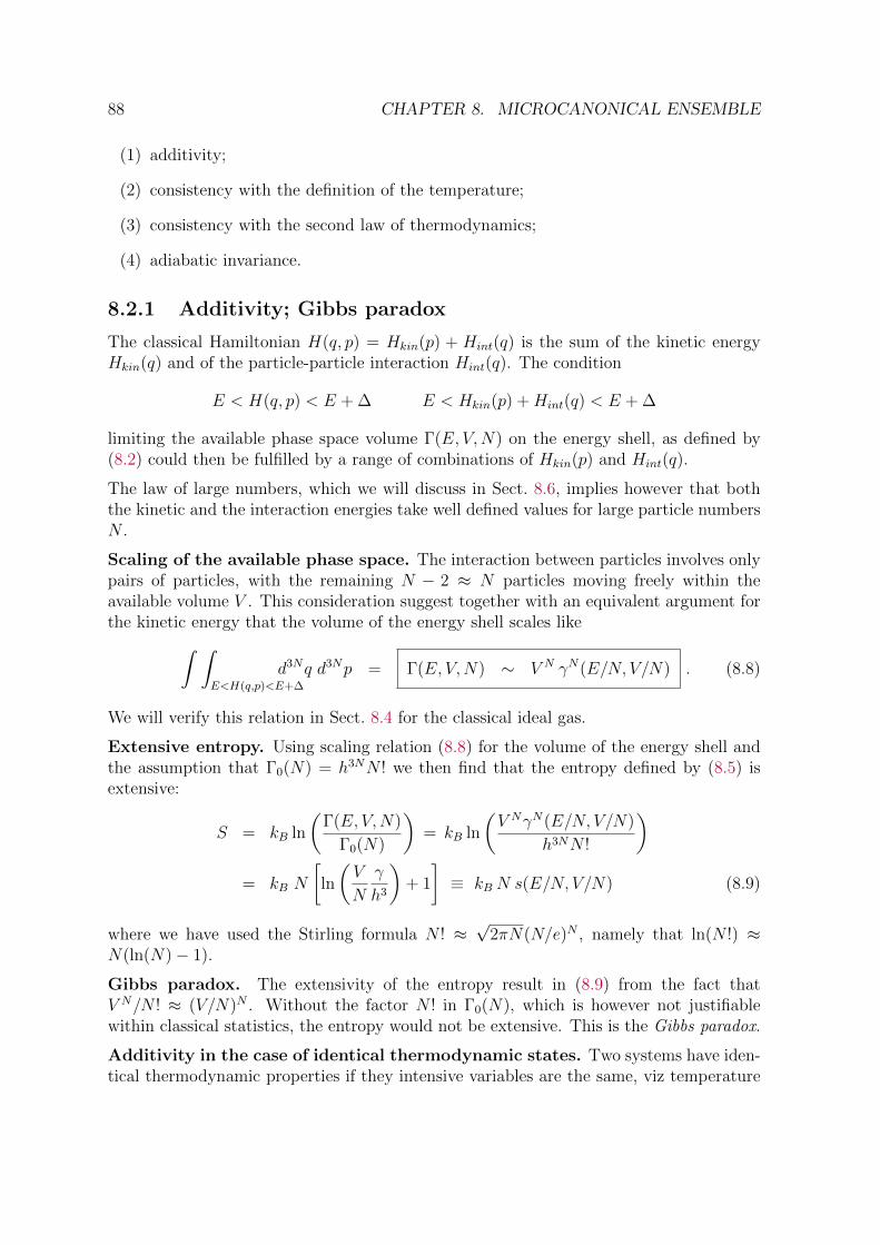
S(E, V,N) = kB (N1 +N2) s(E/N, V/N) = S(E1, V1, N1) + S(E2, V2, N2) ,

where we have used that N = N1 +N2.

Additivity for two systems in thermal contact. Two systems defined by E1, V1,N1 and respectively E2, V2, N2 in thermal contact may allow energy such that the totalenergy E = E1 + E2 is constant. For the argument of the entropy we have then:

Γ(E, V,N)

Γ0(N)=�

E1

Γ(E1, V1, N1)

Γ0(N1)

Γ(E − E1, V2, N2)

Γ0(N2)(8.10)

The law of large numbers tells us that the right-hand-side is sharply peaked at its maxi-mum value E1 = Emax and that the width of the peak has a width scaling with

√Emax.

We hence have

S(Emax) < S(E,N, V ) < kB ln��

Emax

�+ S(Emax) , (8.11)

where the first inequality is due to the fact that a single term is smaller than the sum ofpositive terms. The second inequality in (8.11) results when when one replaces the sumon the r.h.s. of (8.10) by the product of the width

√Emax of the peak and its height.

We have defined in (8.11)

S(Emax) = kB ln

�Γ(Emax, V1, N1) Γ(E − Emax, V2, N2)

Γ0(N1) Γ0(N2)

�,

from which follows that S(E, V,N) = S(E1, V1, N1) + S(E2, V2, N2) . Note that theentropy S(Emax) is extensive and that the term ∼ ln(Emax) in (8.11) is hence negligiblein the thermodynamic limit N → ∞.

8.2.2 Consistency with the definition of the temperature

Two systems with entropies S1 = S(E1, V1, N1) and S2 = S(E2, V2, N2) in thermal contactmay exchange energy in the form of heat, with the total entropy,

0 = dS =∂S1

∂E1

dE1 +∂S2

∂E2

dE1, dE1 = −dE2 , (8.12)

90 CHAPTER 8. MICROCANONICAL ENSEMBLE

becoming stationary at equilibrium. Note that the total energy E1 +E2 is constant. Theequilibrium condition (8.12) implies that there exists a quantity T , denoted temperature,such that

∂S1

∂E1

=1

T=

∂S2

∂E2

. (8.13)

The possibility to define the temperature, as above, is hence a direct consequence of theconservation of the total energy. From the microcanonical definition of the entropy oneonly needs that the entropy is a function only of the internal energy, via the volumeΓ(E, V,N) of the energy shell, and not of the underlying microscopic equation of motion.

8.2.3 Consistency with the second law of thermodynamics

We would like to confirm here that the statistical entropy, defined by (8.5) fulfills thesecond law of thermodynamics

“If an isolated system undergoes a process between two states at equilibrium,the entropy of the final state cannot be smaller than that of the initial state.”

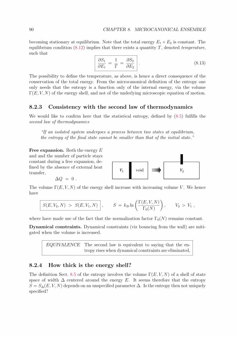
Free expansion. Both the energy Eand and the number of particle staysconstant during a free expansion, de-fined by the absence of external heattransfer,

ΔQ = 0 .

The volume Γ(E, V,N) of the energy shell increase with increasing volume V . We hencehave

S(E, V2, N) > S(E, V1, N) , S = kB ln

�Γ(E, V,N)

Γ0(N)

�, V2 > V1 ,

where have made use of the fact that the normalization factor Γ0(N) remains constant.

Dynamical constraints. Dynamical constraints (viz bouncing from the wall) are miti-gated when the volume is increased.

EQUIVALENCE The second law is equivalent to saying that the en-tropy rises when dynamical constraints are eliminated,

8.2.4 How thick is the energy shell?

The definition Sect. 8.5 of the entropy involves the volume Γ(E, V,N) of a shell of statespace of width Δ centered around the energy E. It seems therefore that the entropyS = SΔ(E, V,N) depends on an unspecified parameterΔ. Is the entropy then not uniquelyspecified?

8.3. CALCULATING WITH THE MICROCANONICAL ENSEMBLE 91

Reference energy. For small Δ we may use the approximation

Γ(E, V,N) ≈ Ω(E)Δ, Ω(E) =∂Φ(E)

∂E, (8.14)

where Ω(E) is the density of states, as defined previously in (8.3). In order to decidewhether a given Δ is small or large we need a reference energy Δ0. One may take f.i.Δ0 ∼ kBT , which corresponds, as shown in Sect. 3.4.1, in order of magnitude to thethermal energy of an individual particle.

Thermodynamic limit. The entropy involves the logarithm of Γ(E, V,N),

ln

�Γ(E, V,N)

Γ0

�= ln

�Ω(E)ΔΔ0

Γ0Δ0

�= ln

�Ω(E)Δ0

Γ0

�

� �� �∝ N

+ ln(Δ/Δ0) ,

where we have taken care the arguments of the logarithms are dimensionless. The keyinsight resulting from this representation is that the exact value of both Δ and Δ0 isirrelevant in the thermodynamic limit N → ∞ as long as

�� ln(Δ/Δ0)�� � N .

Energy quantisation will ensure this condition in quantum statistics.

Shell vs. sphere. We may also considering the limit of large Δ to the extend that wemay substitute the volume Φ(E) for the the volume Γ(E, V,N) of the energy shell,

ln�Γ(E, V,N)

�≈ ln

�Φ(E)

�, (8.15)

where we have disregarded the normalization factor Γ0. The reason that (8.15) holdsstems from the fact that the volume and surface of a sphere with radius R of dimension3N , compare Sect. 8.3.1, scale respectively like R3N and R3N−1. This scaling leads to

ln�Φ(E)

�∼ ln

�R3N

�= 3N ln(R)

ln�Γ(E, V,N)

�∼ ln

�R3N−1Δ

�= (3N − 1) ln(R) + ln(Δ)� �� �

∼ 3N ln(R)

,

which corroborates (8.15). We did not perform here an analysis of the units involved,neglected in particular the reference energy Δ0.

8.3 Calculating with the microcanonical ensemble

In order to perform calculations in statistical physics one proceeds through the followingsteps.

1) Formulation of the Hamilton function

H(q, p) = H(q1, . . . , q3N , p1, . . . , p3N , z) ,

where z is some external parameter, e.g., volume V . H(q, p) specifies the microscopicinteractions.

92 CHAPTER 8. MICROCANONICAL ENSEMBLE

2) Determination of the phase space Γ(E, V,N) and calculation of the density of statesΩ(E, V,N):

Ω(E, V,N) =

�d3Nq

�d3Np δ(E −H(q, p)) .

3) Calculation of the entropy from the volume Φ(E) of the energy sphere:

S(E, V,N) = kB ln

�Φ(E)

Γ0

�.

4) Calculation of P, T, µ:

1

T=

�∂S

∂E

�

V,N

, −µ

T=

�∂S

∂N

�

E,V

,P

T=

�∂S

∂V

�

E,N

.

5) Calculation of the internal energy:

U = �H� = E(S, V,N) .

6) Calculation of other thermodynamic potentials and their derivatives by applicationof the Legendre transformation:

F (T, V,N) = U − TS,

H(S, P,N) = U + PV,

G(T, P,N) = U + PV − TS .

7) One can calculate other quantities than the thermodynamic potentials, for instance,probability distribution functions of certain properties of the system, e.g., mo-menta/velocity distribution functions. If the phase space density of a system ofN particles is given by

ρ(q, p) = ρ(�q1, . . . , �qN , �p1, . . . , �pN) ,

then the probability of finding particle i with momentum �p is

ρi(�p) = �δ (�p− �pi)�

=

�d3q1 . . . d

3qN

�d3p1 . . . d

3pN ρ (�q1, . . . , �qN , �p1, .., �pi, .., �pN) δ (�p− �pi) .

8.3.1 Hyperspheres

Let us calculate for later purposes the volume

Ωn(R) =

��n

i=1 x2i<R2

dnx = RnΩn(1) (8.16)

8.4. THE CLASSICAL IDEAL GAS 93

of a hypersphere of n dimensions and radius P .

Spherical coordinates. We notice that the volume Ωn(1) of the sphere with unity radiusenters the determinant of the Jacobian when transforming via

dnx = dx1 . . . dxn = Ωn(1)nRn−1 dR (8.17)

euclidean to spherical coordinates. This transformation is valid if the integrand dependsexclusively on the radius R.

Gaussian integrals. In order to evaluate (8.16) we make use of the fact that we canrewrite the Gaussian integral

� +∞

−∞dx e−x2

=√π,

� +∞

−∞dx1 . . .

� +∞

−∞dxn e

−(x21+...+x2

N ) = πn/2 .

as

πn/2 =

� ∞

0

e−R2

Ωn(1)nRn−1 dR = nΩn(1)

� ∞

0

e−y y(n−1)/2 dy

2√y

=n

2Ωn(1)

� ∞

0

e−y yn2−1 dy , (8.18)

where we have used (8.17),�

i x2i = R2 ≡ y and that 2RdR = dy.

Gamma function. With the definition

Γ(z) =

� ∞

0

dx xz−1e−x,

of the Γ-function we then obtain from (8.18) that

πn/2 =n

2Ωn(1)Γ(n/2), Ωn(1) =

πn/2

(n/2)Γ(n/2). (8.19)

Note that we did evaluate the volume of a hypersphere for formally dimensionless variablesxi. For later purposes we will need that

Γ(N) = (N − 1)Γ(N − 1), Γ(N) = (N − 1)! (8.20)

whenever the argument of the Γ-function is an integer.

8.4 The classical ideal gas

We consider now the steps given in Sect. 8.3 in order to analyze an ideal gas of N particlesin a volume V , defined by the Hamilton function

H(q, p) =N�

i=1

�p 2i

2m,

94 CHAPTER 8. MICROCANONICAL ENSEMBLE

where m is the mass of the particles.

Phase space volume. We will make use of (8.15), namely that the volume Γ(E, V,N)of the energy sphere

E < H < E +Δ.

can be replaced by the volume of the energy shell,

Φ(E) =

� ��3N

i=1 p2i≤2mE

d3Nq d3Np = V N

��3N

i=1 p2i≤2mE

d3Np

� �� �Ω3N (

√2mE)

, (8.21)

when it comes to calculating the entropy in the thermodynamic limit. We have identifiedthe last integral in (8.21) as the volume of a 3N -dimensional sphere with radius

√2mE.

Using (8.16) and (8.19),

Ω3N(√2mE) = (2mE)3N/2 Ω3N(1), Ω3N(1) =

π3N/2

(3N/2)Γ(3N/2),

we obtain

Φ(E) = V NΩ3N(1)�√

2mE�3N

. (8.22)

8.4.1 Entropy

Using (8.22) we find

S(E, V,N) = kB ln

�Φ(E)

h3NN !

�= kB ln

V N

�√2mE

�3NΩ3N(1)

h3NN !

(8.23)

for the entropy of a classical gas. It is easy to check, that the argument of the logarithmis dimensionless as it should be.

Large N expansion. ForN >> 1, one may use the Stirling formula, N ! ≈√2πN(N/e)N ,

to expand the Γ-function for integer argument as

ln�Γ(N)

�= ln

�(N − 1)!

�

≈ (N − 1) ln(N − 1)− (N − 1)

≈ N ln(N)−N ,

8.4. THE CLASSICAL IDEAL GAS 95

in order to simplify the expression for S(E, V,N). Using (8.19) we perform the followingalgebraic transformations to Ω3N(1):

lnΩ3N(1) = ln

�π

3N2

3N2Γ�3N2

��

=3N

2ln π −

�3N

2ln

�3N

2

�− 3N

2

�

=3N

2ln

2π

3N+

3N

2

= N

�ln

�2π

3N

�3/2

+3

2+O

�lnN

N

��.

We insert this expression in Eq. (8.23) and obtain:

S = kBN

ln

�V (2mE)3/2

h3

�+ ln

�2π

3N

�3/2

+3

2− (lnN − 1)� �� �

lnN !N

. (8.24)

Sackur-Tetrode Equation. Rewriting (8.24) as

S = kBN

�ln

��4πmE

3h2N

�3/2V

N

�+

5

2

�(8.25)

we obtain the Sackur-Tetrode equation.

Equations of state. Now we can differentiate the Sackur-Tetrode equation (8.25) andthus obtain

- the caloric equation of state (3.5) for the ideal gas:

1

T=

�∂S

∂E

�

V,N

= NkB3

2

1

E, E =

3

2NkBT = U

- the thermal equation of state for the ideal gas:

P

T=

�∂S

∂V

�

E,T

=kBN

V, PV = NkBT .

Gibbs Paradox. If we hadn’t considered the factor N ! when working out the entropy,then one would obtain that

Sclassical = kBN

�ln

��4πmE

3h2N

�3/2

V

�+

3

2

�.

96 CHAPTER 8. MICROCANONICAL ENSEMBLE

With this definition, the entropy is non-additive, i.e.,

S(E, V,N) = Ns

�E

N,V

N

�

is not fulfilled, as mentioned already in Sect. 8.2.1. This was realized by Gibbs, who intro-duced the factor N ! and attributed it to the fact that the particles are indistinguishable.

8.5 Fluctuations and correlation functions

We use, as defined in Sect. 7.2.3, the probability distribution function ρM(q, p) in phasespace, which could be evaluated as a time average

ρ(q, p) = limM→∞

1

M

M�

l=1

δ(3N)�q − q(l)

�δ(3N)

�p− p(l)

�

of M measurements of the states (q(l), p(l)) visited along a given trajectory. We havepointed out in (8.1) that ρ(q, p) is uniformly distributed on the energy shell for a micro-canonical ensemble.

Observables. A classical observable B(q, p) corresponds to a function

B(q, p) = B (q1, . . . , q3N , p1, . . . , p3N) ,

phase state. We start with the basic properties.

Expectation value. The average value of B(q, p) is

�B(q, p)� = limM→∞

1

M

M�

l=1

B�q(l), p(l)

�

=

�

Γ

d3Nq d3Np ρ(q, p) B(q, p) .

Variance. The Variance of a function on phase space is

(ΔB)2 =�(B − �B�)2

�=�B2�− �B�2 = σ2

B .

The variance provides information about the fluctuation effects around the average value.

Higher momenta. A momentum of order n is defined generically as

µn = �Bn� .

Probability distribution of an observable. We may define with

ρ(b) =

�d3Nq d3Np ρ(q, p) δ(b− B(q, p)) = �δ(b− B(q, p)� (8.26)

also the probability distribution ρ(b) of the observable B. The expectation value of B isthen given as

�B� =

�db b ρ(b) .

8.5. FLUCTUATIONS AND CORRELATION FUNCTIONS 97

8.5.1 Characteristic function and cumulants

The characteristic function of an observable

ϕB(z) =�eizB

�=

�d3Nq d3Np ρ(q, p) eizB(q,p) . (8.27)

is both a function of the dummy variable∗ z and a functional † of the observable B =B(q, p).

Generating functional. The characteristic function of a random variable B serves as agenerating functional, as it allows via suitable differentions (with respect to the dummyvariable z),

µn =1

indn

dznϕB(z)

���z=0

, ϕB(z) =∞�

n=0

(iz)n

n!µn , (8.28)

to recover the moments µn of underlying probability distribution.

Cummulants. In (8.27) we did expand ϕB(z) in powers of z. Alternatively one mayexpand the logarithm of ϕB(z) in powers of z. One obtains (here without proof)

lnϕB(z) =∞�

n=1

ζn(iz)n

n!= µ1iz − σ2 z

2

2+ . . . . (8.29)

The coefficients

ζ1 = µ1 = �B�ζ2 = σ2 = �B2� − �B�2ζ3 = . . .

are called cumulants.

Extensivity. Cummulant expansions like (8.29) are found in many settings, they form,e.g., the basis of high-temperature expansions. The reason is that cumulants are (incontrast to the moments) consistent with extensivity requirements, f.i. with respect tothe volume V :

�B� ∼ V, �B2� ∼ V 2, ζ2 = �B2� − �B�2 ∼ N .

All cumulants are size-extensive.

8.5.2 Correlations between observables

We define in analogy to (8.26) the joint distribution function ρ(a, b),

ρ(a, b) =�δ(a− A)δ(b− B)

�(8.30)

=

�d3Nq d3Np ρ(q, p) δ

�a− A(q, p)

�δ�b− B(q, p)

�

∗ A dummy variable doesn’t have a physical meaning. It solely serves for computational purposes.† A functional is a function of another function.

98 CHAPTER 8. MICROCANONICAL ENSEMBLE

of two observables A = A(q, p) and B = B(q, p).

Cross correlation function. The joint distribution function ρ(a, b) allows to investigatethe cross correlations

CAB =�(A− < A >)(B− < B >)

�(8.31)

=

�da

�db ρ(a, b)

�a− �A�

��b− �B�

�

between A and B.

Uncorrelated variables. Two observable are uncorrelated if they are statistically inde-pendent. The joint distribution factorizes is this case,

ρ(a, b) = ρA(a)ρB(b) .

The cross correlations vanish consequently:

CAB =��A− �A�

��B − �B�

��

=�A− �A�

� �B − �B�

�

= 0 .

8.6 Central limit theorem

Consider M statistically independent observables Bm(q, p). The central limit theoremstates then that the probability density of the observable

B(q, p) =M�

m=1

Bm(q, p)

is normal distributed with an extensive mean �B� ∼ M and with the width proportionalto

√M .

8.6.1 Normal distribution

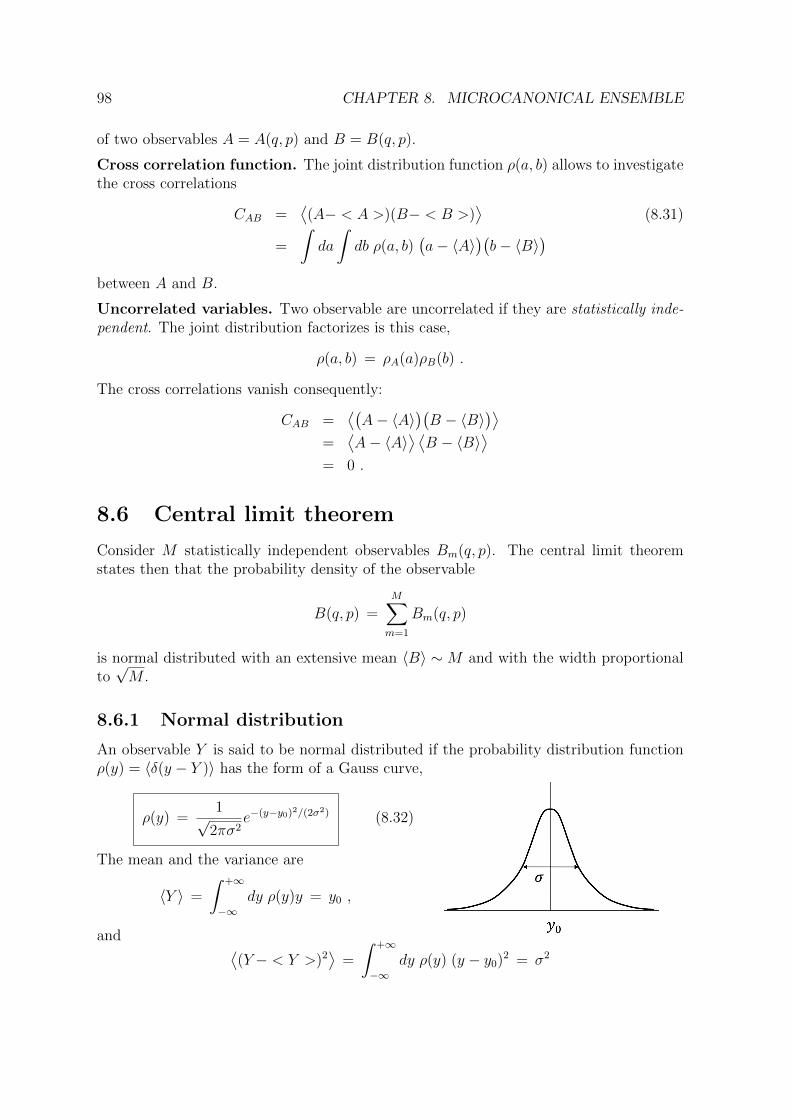
An observable Y is said to be normal distributed if the probability distribution functionρ(y) = �δ(y − Y )� has the form of a Gauss curve,

ρ(y) =1√2πσ2

e−(y−y0)2/(2σ2) (8.32)

The mean and the variance are

�Y � =

� +∞

−∞dy ρ(y)y = y0 ,

and�(Y− < Y >)2

�=

� +∞

−∞dy ρ(y) (y − y0)

2 = σ2

8.6. CENTRAL LIMIT THEOREM 99

respectively. The even moments of the normal distribution are finite,

�Y 2n

�=

(2n)!

2nn!σ2n ,

with the odd moments �Y 2n+1� = 0 vanishing due to the reflection symmetry with respectto the mean y0.

Characteristic function. The characteristic function of a normal distribution is also aGauss function:

f(z) =�eizY

�=

� +∞

−∞dy eizyρ(y) = eizy0e−

12z2σ2

. (8.33)

For the proof consider the overall exponent

izy − (y − y0)2

2σ2= −y2 − 2y0y − 2izyσ2 + y20

2σ2

= −(y − y0 − izσ2)2

2σ2+ izy0 −

1

2z2σ2 .

8.6.2 Derivation of the central limit theorem

For the derivation of the central limit we define a variable Y as

Y ≡ 1√M

�X1 +X2 + . . .+XM

�,

where X1, X2, . . ., XM are M mutually independent variables such that �Xi� = 0 forconvenience.

Characteristic function of independent variables. We make now use of the fact,that the characteristic function of the sum independent variables, such as for Y , factorizes:

�e−izY

�=

�e−iz(X1+X2+...+XM )/

√M�

=

�M�

j=1

e−izXj/√M

�

=M�

j=1

�e−izXj/

√M�

.

Using the representation

Aj(z/√M) ≡ ln

�e−izXj/

√M�

(8.34)

for the logarithm of the characteristic function �exp(−izXj/√M)� of the individual ran-

dom variables we then find

�e−izY

�= exp

�M�

j=1

Aj(z/√M)

�. (8.35)

100 CHAPTER 8. MICROCANONICAL ENSEMBLE

Large M expansion. If M is a large number, Aj(z/√M) can be expanded as

Aj(z/√M) � Aj(0) +

z2

2MA��

j (0) +z3

MO(M−1/2) . (8.36)

Here, the first-order term A�j(0) in z vanishes because it is proportional to �Xj� = 0.

Variance. The quadratic term is (8.36) is obtained by differentiating (8.34):

A��j (0) = −

�X2

j

�.

Substituting now (8.36) into (8.34) one obtains with

�e−izY

�= exp

�−1

2z2σ2 +O

�1√M

��, σ2 ≡ 1

M

M�

j=1

�X2

j

�(8.37)

the proof of the central limit theorem. Compare (8.37) with (8.33).

Finite mean. The expectation values add,

�Y � =M�

j=1

< Xj > /√M ,

when the means �Xj� �= 0 of the individual variables are finite. Y − �Y � is then normaldistributed.

Binomial distribution. As a first example we consider the binomial distribution in thelimit of a large number of draws (flipping of a coin):

n =N�

i=1

ni ni =

�1 with probability p0 with probability 1− p

The probability ρN(n) to get a one n times out of N coin flip is then

ρN(n) =

�Nn

�pn(1− p)N−n . (8.38)

The central limit theorem predicts that

limN→∞

ρN(n) → 1√2πNσ2

e−(n−<n>)2/2Nσ2

, (8.39)

where

σ2 =1

N

N�

i=1

��n2i

�− �ni�2

�= p(1− p)

is the variance of a single coin flip.

8.6. CENTRAL LIMIT THEOREM 101

0 0.2 0.4 0.6 0.8 1

x0

0.01

0.02

pro

bab

ilit

y d

ensi

ties

flat, N=1

Gaussianflat, N=3

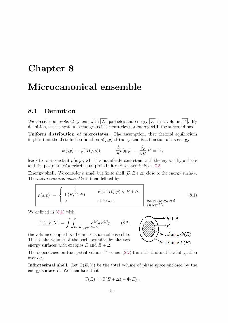
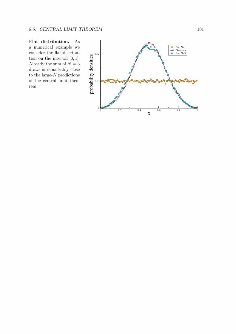
Flat distribution. Asa numerical example weconsider the flat distribu-tion on the interval [0, 1].Already the sum of N = 3draws is remarkably closeto the large-N predictionsof the central limit theo-rem.

102 CHAPTER 8. MICROCANONICAL ENSEMBLE