
Asymptotic Bode Plot & Lead-Lag Compensatormsang/BodePlot.pdf · Asymptotic Bode Plot & Lead-Lag...
8
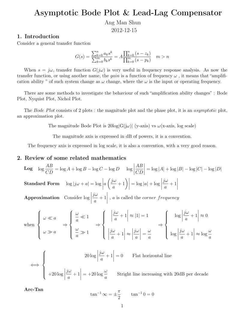
Asymptotic Bode Plot & Lead-Lag Compensator Ang Man Shun 2012-12-15 1. Introduction Consider a general transfer function G(s)= ∑ n k=0 a k s k ∑ m k=0 b k s k = A ∏ n k=0 (s − z k ) ∏ m k=0 (s − p k ) m>n When s = jω, transfer function G(jω) is very useful in frequency response analysis. As now the transfer function, or using another name, the gain is a function of frequency ω , it means that “amplifi- cation ability ” of such system change as ω change, where the ω is the input or operating frequency. There are some methods to investigate the behaviour of such “amplification ability changes” : Bode Plot, Nyquist Plot, Nichol Plot. The Bode Plot consists of 2 plots : the magnitude plot and the phase plot, it is an asymptotic plot, an approximation plot. The magnitude Bode Plot is 20log|G(jω)| (y-axis) vs ω(x-axis, log scale) The magnitude axis is expressed in dB of powers, it is a convention. The frequency axis is expressed in log scale, it is also a convention, with a very good reason. 2. Review of some related mathematics Log log AB CD = log A + log B − log C − log D log AB CD = log |A| + log |B|− log |C |− log |D| Standard Form log |jω + a| = log a ( jω a +1 ) = log |a| + log jω a +1 1 Approximation Consider log jω a +1 , a is called the corner frequency when ω ≪ a ω ≫ a ⇒ ω a ≪ 1 ω a ≫ 1 ⇒ jω a +1 ≈|1| =1 jω a +1 ≈ jω a = ω a ⇒ log jω a +1 ≈ 0 log jω a +1 ≈ log ω a ⇐⇒ 20 log jω a +1 =0 Flat horizontal line +20 log jω a +1 = +20 log ω a Stright line increasing with 20dB per decade Arc-Tan tan -1 ∞ = ± π 2 tan -1 0=0
Transcript of Asymptotic Bode Plot & Lead-Lag Compensatormsang/BodePlot.pdf · Asymptotic Bode Plot & Lead-Lag...
Asymptotic Bode Plot & Lead-Lag CompensatorAng Man Shun
2012-12-151. IntroductionConsider a general transfer function
G(s) =
∑nk=0 aks
k∑mk=0 bks
k= A
∏nk=0 (s− zk)∏mk=0 (s− pk)
m > n
When s = jω, transfer function G(jω) is very useful in frequency response analysis. As now thetransfer function, or using another name, the gain is a function of frequency ω , it means that “amplifi-cation ability ” of such system change as ω change, where the ω is the input or operating frequency.
There are some methods to investigate the behaviour of such “amplification ability changes” : BodePlot, Nyquist Plot, Nichol Plot.
The Bode P lot consists of 2 plots : the magnitude plot and the phase plot, it is an asymptotic plot,an approximation plot.
The magnitude Bode Plot is 20log|G(jω)| (y-axis) vs ω(x-axis, log scale)
The magnitude axis is expressed in dB of powers, it is a convention.
The frequency axis is expressed in log scale, it is also a convention, with a very good reason.
2. Review of some related mathematics
Log logAB
CD= logA+ logB − logC − logD log
∣∣∣∣ABCD
∣∣∣∣ = log |A|+ log |B| − log |C| − log |D|
Standard Form log |jω + a| = log
∣∣∣∣a(jω
a+ 1
)∣∣∣∣ = log |a|+ log
∣∣∣∣jωa + 1
∣∣∣∣
1
Approximation Consider log
∣∣∣∣jωa + 1
∣∣∣∣ , a is called the corner frequency
when
ω ≪ a
ω ≫ a
⇒
ω
a≪ 1
ω
a≫ 1
⇒
∣∣∣∣jωa + 1
∣∣∣∣ ≈ |1| = 1
∣∣∣∣jωa + 1
∣∣∣∣ ≈ ∣∣∣∣jωa∣∣∣∣ = ω
a
⇒
log
∣∣∣∣jωa + 1
∣∣∣∣ ≈ 0
log
∣∣∣∣jωa + 1
∣∣∣∣ ≈ logω
a
⇐⇒
20 log
∣∣∣∣jωa + 1
∣∣∣∣ = 0 Flat horizontal line
+20 log
∣∣∣∣jωa + 1
∣∣∣∣ = +20 logω
aStright line increasing with 20dB per decade
Arc-Tantan−1∞ = ±π
2tan−1 0 = 0

3. ExampleFor example, consider a degree 1 transfer function with 5 zeros and poles.
G(s) =A (s+ a) (s+ b)
(s+ c) (s+ d) (s+ e)
Where −a , −b are zeros, −c , −d , −e are poles.
Before doing the Bode Plot analysis, turn the transfer function into “Standard Form”
G(s) =Aab
cde·
(sa+ 1
)(sb+ 1
)(sc+ 1
)(sd+ 1
)(se+ 1
) =k(sa+ 1
)(sb+ 1
)(sc+ 1
)(sd+ 1
)(se+ 1
) k =Aab
cde
The magnitude (in dB of powers) is thus
20 log |G(s)| = 20 log
∣∣∣∣∣∣k(sa+ 1
)(sb+ 1
)(sc+ 1
)(sd+ 1
)(se+ 1
)∣∣∣∣∣∣
= 20 log |k|+ 20 log∣∣∣sa+ 1
∣∣∣+ 20 log∣∣∣sb+ 1
∣∣∣− 20 log∣∣∣sc+ 1
∣∣∣− 20 log∣∣∣sd+ 1
∣∣∣− 20 log∣∣∣se+ 1
∣∣∣The Bode Plot is thus
2
4. For more general case
• The Effect of DC term : a horizontal line
• The Effect of a pole at α : For ω < α , no effect (since it is in log scale ! ) , for ω > α , it goesdown at a rate of 20dB per decade.
• The Effect of a zero at β : For ω < β , no effect (since it is in log scale !) , for ω > β , it goes upat a rate of 20dB per decade.

More General
• For a simple , 1st order pole at α : For ω < α , no effect, for ω > α , it goes down at a rate of1 · 20dB per decade.
• For a nth order pole at β : For ω < α , no effect, for ω > α , it goes down at a rate of n20 dB perdecade.
• In same logic, a mth order zero at γ will give a increasing straight with slope of m20dB per decade, starting at ω = γ
5. Summary of Magnitude Plot
The algorithm to draw Magnitude Bode Plot is
• Turn the transfer function into standard form (s+ a) → a(s
a+ 1)
• Find all the corner frequency
• For zeros, the lines go up. For poles, the lines go down.
• The slope of the line is 20dB·the degree of the pole/zero.
3
6. Phase Plot
Consider (jω + a), the angle of this term is tan−1 ω
a
When ω ≪ a ( The axis is in scale of decade, i.e. 10 time)
ω = 0.1a tan−1 ω
a= tan−1(0.1) = 5.7o
ω = 0.01a tan−1 ω
a= tan−1(0.01) = 0.57o
When ω ≫ a ( The axis is a log scale, so consider a decade , i.e. 10 time )
ω = 10a tan−1 ω
a= tan−1(10) = 84.3o
ω = 100a tan−1 ω
a= tan−1(100) = 89.4o
So in general,
tan−1 ω
a≈
0o ω ≪ a
90o ω ≫ a

7. Examples G(s) =K0
T0s+ 1K0, T0 > 0
20 log |G(jω)| = 20 log |K0| − 20 log
∣∣∣∣ jω1/T0
+ 1
∣∣∣∣∠G(jω) = ∠K0︸︷︷︸
0
−∠(
jω1/T0
+ 1
)Let K = 4 , T0 = 0.5
G(s) =4
1
2s+ 1
• 20 log |4| = 27
• Corner Frequenct in magnitude plot : 0.5
• Corner Frequency in phase plot : 0.05 and 5
4
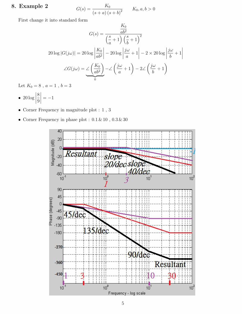
8. Example 2G(s) =
K0
(s+ a) (s+ b)2K0, a, b > 0
First change it into standard form
G(s) =
K0
ab2(sa+ 1
)(sb+ 1
)2
20 log |G(jω)| = 20 log
∣∣∣∣K0
ab2
∣∣∣∣− 20 log
∣∣∣∣jωa + 1
∣∣∣∣− 2× 20 log
∣∣∣∣jωb + 1
∣∣∣∣∠G(jω) = ∠
(K0
ab2
)︸ ︷︷ ︸
0
−∠(jω
a+ 1
)− 2∠
(jω
b+ 1
)
Let K0 = 8 , a = 1 , b = 3
• 20 log
∣∣∣∣89∣∣∣∣ = −1
• Corner Frequency in magnitude plot : 1 , 3
• Corner Frequency in phase plot : 0.1&10 , 0.3&30
5
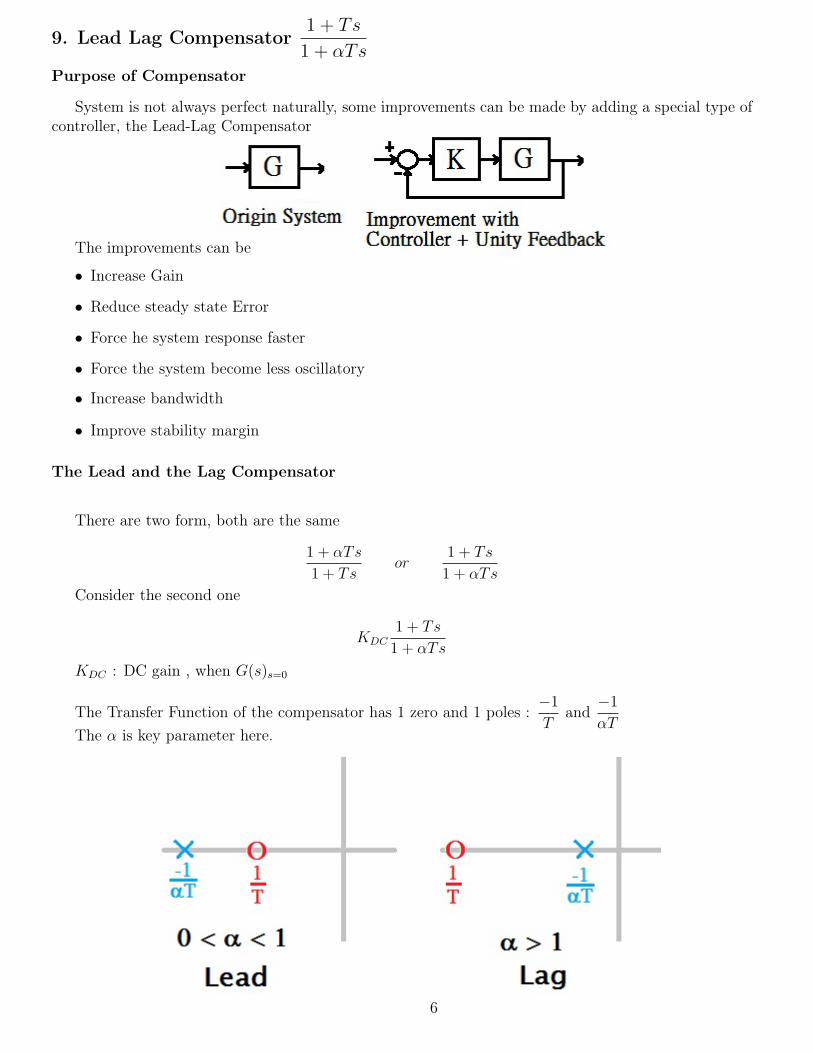
9. Lead Lag Compensator1 + Ts
1 + αTs
Purpose of Compensator
System is not always perfect naturally, some improvements can be made by adding a special type ofcontroller, the Lead-Lag Compensator
The improvements can be
• Increase Gain
• Reduce steady state Error
• Force he system response faster
• Force the system become less oscillatory
6
• Increase bandwidth
• Improve stability margin
The Lead and the Lag Compensator
There are two form, both are the same
1 + αTs
1 + Tsor
1 + Ts
1 + αTs
Consider the second one
KDC1 + Ts
1 + αTs
KDC : DC gain , when G(s)s=0
The Transfer Function of the compensator has 1 zero and 1 poles :−1
Tand
−1
αTThe α is key parameter here.

Consider their Bode Plot
K(s) = KDC1 + Ts
1 + αTs
Standard Form
K(s) = KDC
1 +s
1/T
1 +s
1/αT
20 log |K(jω)| = 20 log |KDC |+ 20 log
∣∣∣∣1 + jω1/T
∣∣∣∣− 20 log
∣∣∣∣1 + jω
1/αT
∣∣∣∣∠K(jω) = ∠KDC︸ ︷︷ ︸
0
+∠(1 + j
ω1/T
)− ∠
(1 + j
ω1/αT
)
• Corner frequency of magnitude plot :1
T,
1
αT
• Corner frequency of phase plot :1
10T&
10
Tand
1
10αT&
10
αT
7
• Denote1
T= a
1
αT= b
• The following Bode Plot ignore the DC part (Assume KDC = 1)
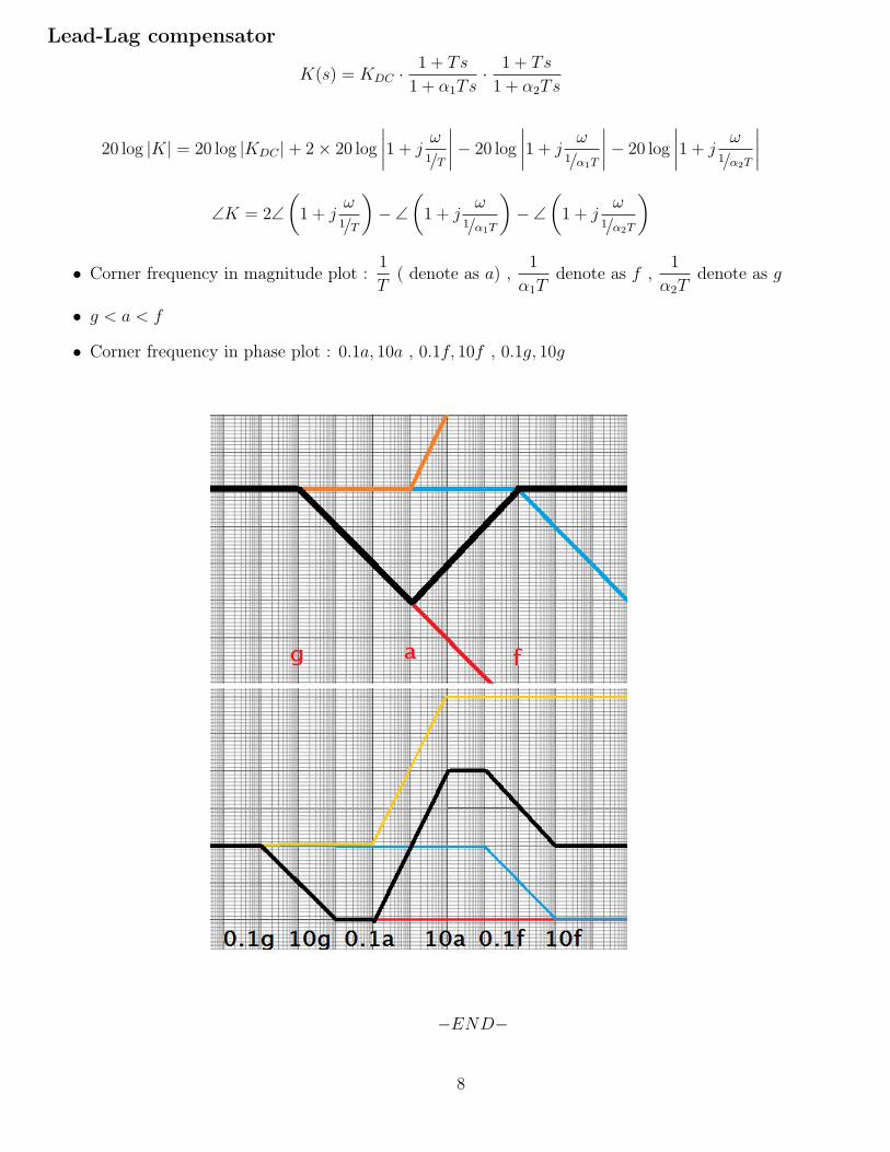
Lead-Lag compensator
K(s) = KDC · 1 + Ts
1 + α1Ts· 1 + Ts
1 + α2Ts
20 log |K| = 20 log |KDC |+ 2× 20 log
∣∣∣∣1 + jω1/T
∣∣∣∣− 20 log
∣∣∣∣1 + jω
1/α1T
∣∣∣∣− 20 log
∣∣∣∣1 + jω
1/α2T
∣∣∣∣∠K = 2∠
(1 + j
ω1/T
)− ∠
(1 + j
ω1/α1T
)− ∠
(1 + j
ω1/α2T
)
• Corner frequency in magnitude plot :1
T( denote as a) ,
1
α1Tdenote as f ,
1
α2Tdenote as g
• g < a < f
• Corner frequency in phase plot : 0.1a, 10a , 0.1f, 10f , 0.1g, 10g
8
−END−
![Biological Research in India - · PDF fileRamachandran plot or a [φ,ψ] plot developed in 1963 by G. N. Ramachandran, C. ... biotechnology, bioinformatics, and the various ‘omics’](https://static.fdocument.org/doc/165x107/5ab3b6597f8b9a1d168ea056/biological-research-in-india-plot-or-a-plot-developed-in-1963-by-g-n.jpg)


![Least Squares Optimization and Gradient Descent Algorithm · 2019. 11. 21. · SCATTER PLOT Plot all (X i, Y i) pairs, and plot your learned model !4 0 20 40 60 0 20 40 60 X Y [WF]](https://static.fdocument.org/doc/165x107/6124df642da9ad37a74372ef/least-squares-optimization-and-gradient-descent-algorithm-2019-11-21-scatter.jpg)