
6. Stability of SISO Feedback Systems - UMass...
24
2/15/2005 6-1 Copyright ©2005 (Yossi Chait) 6. Stability of SISO Feedback Systems Let F(s) = N(s)/D(s), N & D co-prime polynomials. Let Γ(s) be a closed contour in the s-plane. Assume F(s) has no zeros or poles with values ∂Γ. The Principle of the Argument states that as s traces ∂Γ once counterclockwise, F(s) traces a closed counter in the s-plane. Moreover, z = N + p where • p = no. of poles of F(s) inside Γ(s), • z = no. of zeros of F(s) inside Γ(s), • N = no. of counterclockwise origin encirclements by the plot of F(s) (<0 if CCW, >0 if CW).
Transcript of 6. Stability of SISO Feedback Systems - UMass...
2/15/2005 6-1 Copyright ©2005 (Yossi Chait)
6. Stability of SISO Feedback Systems
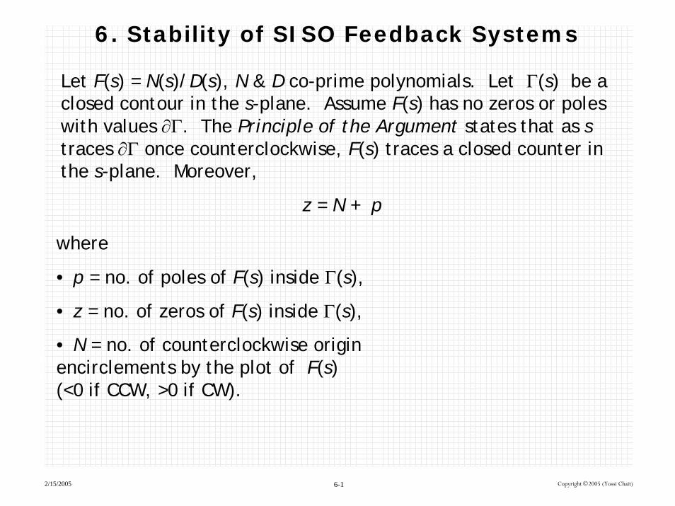
Let F(s) = N(s)/D(s), N & D co-prime polynomials. Let Γ(s) be a closed contour in the s-plane. Assume F(s) has no zeros or poles with values ∂Γ. The Principle of the Argument states that as s traces ∂Γ once counterclockwise, F(s) traces a closed counter in the s-plane. Moreover,
z = N + p
where
• p = no. of poles of F(s) inside Γ(s),
• z = no. of zeros of F(s) inside Γ(s),
• N = no. of counterclockwise origin encirclements by the plot of F(s) (<0 if CCW, >0 if CW).

2/15/2005 6-2 Copyright ©2005 (Yossi Chait)
6.1. Nyquist Stability Criterion
A simply application of the Principle of the Argument with F(s) the open-loop transfer function of a closed-loop system and Γ(s) the closed right-half s-plane. Assume L(s) has no poles on the imaginary axis and no unstable pole/zero cancellation. For the feedback system shown below:
The characteristic equation is 1 + CPH(s) = 0. The open-loop transfer function here is L(s) = CPH(s).
∑−
R YC P
H
2/15/2005 6-3 Copyright ©2005 (Yossi Chait)
6.2. Properties of Θ
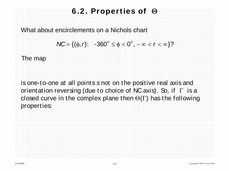
What about encirclements on a Nichols chart
= φ ≤ φ < − ∞ < < ∞{( , ): -360 0 , }?NC r r
The map
is one-to-one at all points s not on the positive real axis and orientation reversing (due to choice of NC axis). So, if Γ is a closed curve in the complex plane then Θ(Γ) has the following properties:
2/15/2005 6-4 Copyright ©2005 (Yossi Chait)
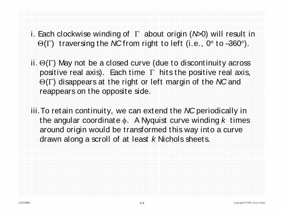
i. Each clockwise winding of Γ about origin (N>0) will result in Θ(Γ) traversing the NC from right to left (i.e., 0° to –360°).
ii.Θ(Γ) May not be a closed curve (due to discontinuity across positive real axis). Each time Γ hits the positive real axis, Θ(Γ) disappears at the right or left margin of the NC and reappears on the opposite side.
iii.To retain continuity, we can extend the NC periodically in the angular coordinate φ. A Nyquist curve winding k times around origin would be transformed this way into a curve drawn along a scroll of at least k Nichols sheets.

2/15/2005 6-5 Copyright ©2005 (Yossi Chait)
6.3. Evaluating Stability using Nichols Plots
Assume the loop transmission, L(s), is a product of a rational (proper or strictly proper) function and a pure time delay. Further assume that no unstable pole/zero cancellations take place in L(s).
We consider a standard Nyquist contour, with right jω-axis indentations as necessary to account for imaginary axis poles ofL(s) is shown below.
x
A standard continuous-time Nyquist contour.

2/15/2005 6-6 Copyright ©2005 (Yossi Chait)
Definition. The Nyquist plot of L(s) is said to have a crossing if it intersects the negative part of the real axis, Re[L(s)] < -1. The sign of the crossing is either positive or negative, depending on the direction of the plot at the crossing point.
Crossings and corresponding signs in the complex plane, Nichols and Bode plots are shown below.

2/15/2005 6-7 Copyright ©2005 (Yossi Chait)
The following is our Nichols plot stability criterion. Let p denote the total number (counting multiplicity) of the unstable poles of L(s) inside the Nyquist contour.
Criterion 1. The feedback system is stable if:
•The single-sheeted Nichols plot of L(s) does not intersect the point q := (-180°, 0dB), and the net sum of its crossings of the ray R0 := {(φ,r): φ = -180°, r > 0dB} is equal to -p; or
•The multiple-sheeted Nichols plot of L(s) does not intersect any of the points (2k+1)q, k = 1,…, and the net sum of its crossings of the rays R0 + 2kq is equal to -p.
2/15/2005 6-8 Copyright ©2005 (Yossi Chait)
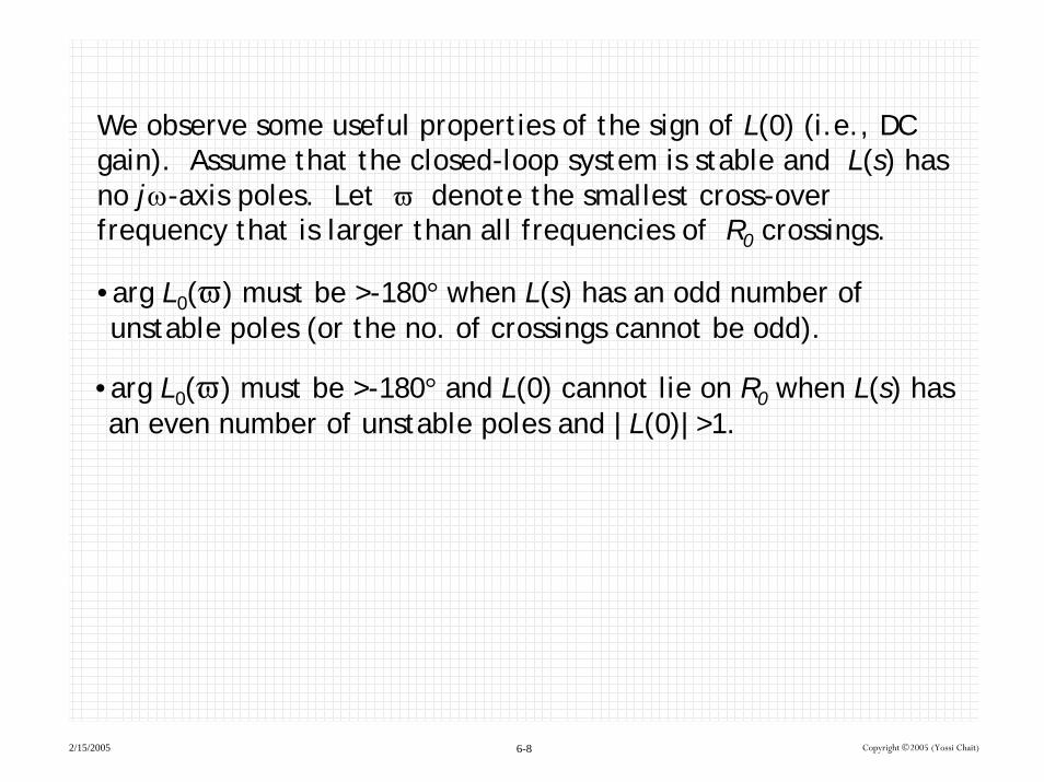
We observe some useful properties of the sign of L(0) (i.e., DC gain). Assume that the closed-loop system is stable and L(s) has no jω-axis poles. Let ϖ denote the smallest cross-over frequency that is larger than all frequencies of R0 crossings.
•arg L0(ϖ) must be >-180° when L(s) has an odd number of unstable poles (or the no. of crossings cannot be odd).
•arg L0(ϖ) must be >-180° and L(0) cannot lie on R0 when L(s) has an even number of unstable poles and |L(0)|>1.

2/15/2005 6-9 Copyright ©2005 (Yossi Chait)
6.4. Examples
Example 1. Consider a unity feedback system that has the following stable open-loop function
The Nyquist plot and its version on a multiple-sheeted Nichols chart are shown for k = 3000.

2/15/2005 6-10 Copyright ©2005 (Yossi Chait)
Nyquist Diagram
Real Axis
Imag
inar
y Ax
is
0 10 20 30 40 50 60
-30
-20
-10
0
10
20
30
0
0
-300 -200 -100 0 100 200 300
-80
-60
-40
-20
0
20
40
Phase (degrees)
Mag
nitu
de (d
B)
8-
-270
• CW direction in complex plane becomes CCW in NC (property i in Section 6.2.).
• For strictly proper functions, L(s) = 0 at the semi-infinite circle portion of the Nyquist contour. On an NC, this is represented by a horizontal segment at -∞ dB starting at L(j∞) and ending at L(-j∞). The width of the segment is equal to (no. of poles - no. of zeros)×180°.
• There’s a LEFT turn at point B’. Why?

2/15/2005 6-11 Copyright ©2005 (Yossi Chait)
-300 -200 -100 0 100 200 300
-80
-60
-40
-20
0
20
40
Phase (degrees)
Mag
nitud
e (d
B)
8-
-350 -300 -250 -200 -150 -100 -50 0
-80
-60
-40
-20
0
20
40
Phase (degrees)
Mag
nitud
e (d
B)
8-
Single-sheeted plot. Multiple-sheeted plot.

2/15/2005 6-12 Copyright ©2005 (Yossi Chait)
What about stability?
From Criterion 1, since the system is open-loop stable (p = 0), we must reduce the gain (i.e., shift the plot down vertically) to eliminate any crossings. If we reduce the gain by 9.5 dB (a factor of 3 approximately), the plot will be just below the rays R0 and R1. Hence, we conclude that the closed-loop system is stable if k<1000.
2/15/2005 6-13 Copyright ©2005 (Yossi Chait)
-350 -300 -250 -200 -150 -100 -50 0
-80
-60
-40
-20
0
20
40
Phase (degrees)
Mag
nitud
e (d
B)
-100
9.5 dB
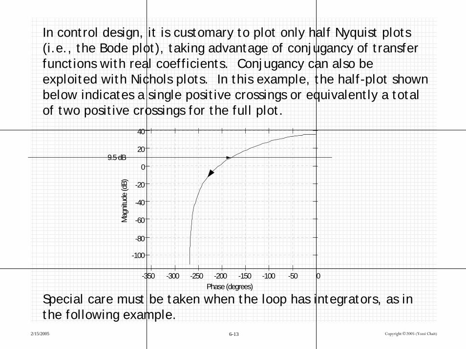
In control design, it is customary to plot only half Nyquist plots (i.e., the Bode plot), taking advantage of conjugancy of transfer functions with real coefficients. Conjugancy can also be exploited with Nichols plots. In this example, the half-plot shown below indicates a single positive crossings or equivalently a total of two positive crossings for the full plot.
Special care must be taken when the loop has integrators, as in the following example.

2/15/2005 6-14 Copyright ©2005 (Yossi Chait)
-350 -300 -250 -200 -150 -100 -50 0
-150
-100
-50
0
Phase (degrees)
Mag
nitud
e (d
B)
8-
8+
Example 2. Consider a unity feedback system that has the following stable open-loop function
The plot on a single-sheeted Nichols chart is shown below for k = 1.
2/15/2005 6-15 Copyright ©2005 (Yossi Chait)
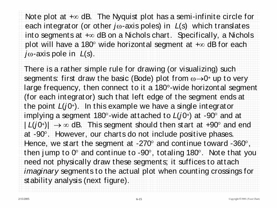
Note plot at +∞ dB. The Nyquist plot has a semi-infinite circle for each integrator (or other jω-axis poles) in L(s) which translates into segments at +∞ dB on a Nichols chart. Specifically, a Nichols plot will have a 180° wide horizontal segment at +∞ dB for each jω-axis pole in L(s).
There is a rather simple rule for drawing (or visualizing) such segments: first draw the basic (Bode) plot from ω→0+ up to very large frequency, then connect to it a 180°-wide horizontal segment (for each integrator) such that left edge of the segment ends atthe point L(j0+). In this example we have a single integrator implying a segment 180°-wide attached to L(j0+) at -90° and at |L(j0+)| → ∞ dB. This segment should then start at +90° and end at -90°. However, our charts do not include positive phases. Hence, we start the segment at -270° and continue toward -360°, then jump to 0° and continue to -90°, totaling 180°. Note that you need not physically draw these segments; it suffices to attach imaginary segments to the actual plot when counting crossings for stability analysis (next figure).
2/15/2005 6-16 Copyright ©2005 (Yossi Chait)
-350 -300 -250 -200 -150 -100 -50 0
-150
-100
-50
0
Phase (degrees)
Mag
nitud
e (d
B)
8+
’
Single-sheeted plot.
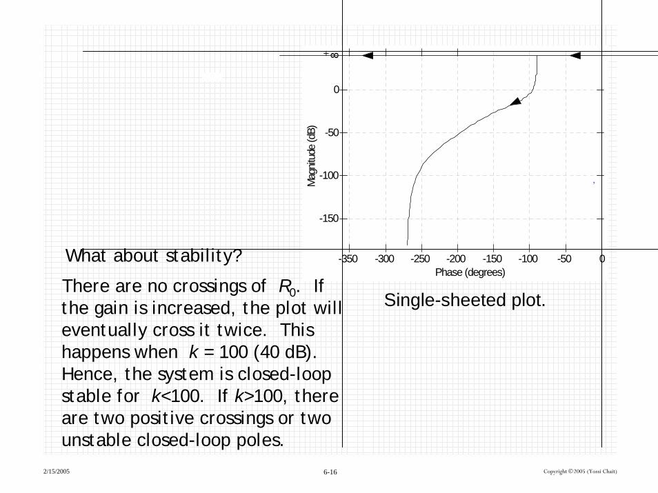
What about stability?
There are no crossings of R0. If the gain is increased, the plot will eventually cross it twice. This happens when k = 100 (40 dB). Hence, the system is closed-loop stable for k<100. If k>100, there are two positive crossings or two unstable closed-loop poles.
2/15/2005 6-17 Copyright ©2005 (Yossi Chait)
In certain cases with poles on the jω-axis, the plot may appear to be tangential to R0 in which case it may not be clear how to count crossings. For example, consider the open-loop function
( ) , 0.2( 1)
kL s k
s s= >
+
As ω→0, ∠L(jω) → -180° and |L(jω)| → ∞. To correctly count any crossings, you need to realize that in fact L(jω) does not lie on R0 at infinity, it is only tangential to it. Specifically, here
Although the real part is at -∞, there is always a non-zero imaginary part as well (of course it is much smaller in magnitude compared to the real part). Hence, the plot does not lie on the ray R0 as ω→0+ and it is possible to count crossing. Another way to interpret the type of crossing is by figuring the phase at ω→0+.

2/15/2005 6-18 Copyright ©2005 (Yossi Chait)
A
B
C
D
E Fx
Nichols Chart
Open-Loop Phase (deg)
Ope
n-Lo
op G
ain
(dB
)
-360 -270 -180 -90 0 90 180 270 360 450 540-40
-30
-20
-10
0
10
20
30
40
-90°
Nichols plot
-3 -2.5 -2 -1.5 -1 -0.5 0 0.5 1-2
-1.5
-1
-0.5
0
0.5
1
1.5
2Root Locus
Real Axis
Imag
inar
y A
xis
Root locus

2/15/2005 6-19 Copyright ©2005 (Yossi Chait)
6.5. Robust Stability Criterion1,2
In many physical situations, the actual plant dynamics are knownto belong to a set (family) of plants P. The notion of robust stability in QFT amounts to checking stability using one nominal loop, where P0(s)∈P is termed the nominal plant, and then demonstrating stability of the whole set P by some argument involving the nature of P. This property is commonly referred to as robust stability.
1. Jayasuriya, S., 1993, “Frequency domain design for robust performance under parametric, unstructured, or mixed uncertainties,” ASME J. of Dynamic Systems, Measurement, and Control, Vol. 115, pp. 439-451.
2. Cohen, N., et al., “Stability analysis using Nichols charts”, Int. J. Robust and Nonlinear Control, Vol 4(3), pp. 3-20, 1994.
2/15/2005 6-20 Copyright ©2005 (Yossi Chait)
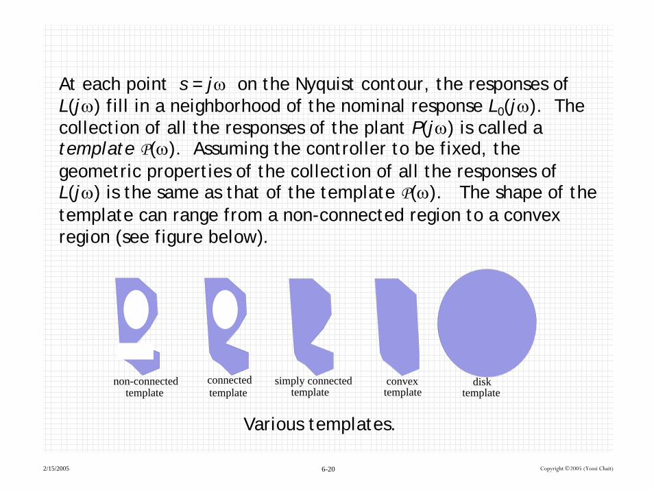
At each point s = jω on the Nyquist contour, the responses of L(jω) fill in a neighborhood of the nominal response L0(jω). The collection of all the responses of the plant P(jω) is called a template P(ω). Assuming the controller to be fixed, the geometric properties of the collection of all the responses of L(jω) is the same as that of the template P(ω). The shape of the template can range from a non-connected region to a convex region (see figure below).
connectedtemplate
convexsimply connectedtemplate
disknon-connectedtemplate template template
Various templates.
2/15/2005 6-21 Copyright ©2005 (Yossi Chait)
For design purposes, one typically enlarges the template into a simply connected region (roughly speaking, it is made of a single “piece” and has no holes). Another possibility is to define the template as the convex hull of the region (in a convex set any two points in the set can be connected via a line). The most conservative, yet most computationally tractable, approachwould be to turn the region into a disk (non-parametric model).
As we traverse the Nyquist contour, the union of these templatesis called the Nichols envelope. Note that templates unify the way QFT treats uncertainty since parametric, non-parametric or mixed uncertainty plant models all have a similar frequency response representation. If your template has holes, the Toolbox algorithms will, roughly speaking, automatically “fill in” and assume that no holes exist.

2/15/2005 6-22 Copyright ©2005 (Yossi Chait)
The following is the Nichols chart robust stability criterion used in QFT. The loop transfer function L(s) is assumed to belong to a set L. In addition to the trivial assumption of no unstable (including jω-axis) pole/zero cancellation in any L(s) in the set, the criterion requires that L belongs to one of the following:
Group A: (1) L(s) is strictly proper, (2) the uncertain parameters belong to a compact and simple connected set, (3) the coefficients of the numerator and denominator of L(s) depend continuously on the uncertain parameters, and (4) the coefficients of the highest degree s terms in the numerator and denominator of L(s) cannot vanish.
Group B: (1) at each fixed frequency, the responses of all L(jω) form a simple-connected set in the complex plane, and (2) the number of unstable poles in L(s) is fixed.

2/15/2005 6-23 Copyright ©2005 (Yossi Chait)
Criterion 2. Assume that the uncertain set L belongs to one of the above groups. Let L0(s) = CP0(s)∈L denote the nominal loop. The feedback system is robust stable if:
The nominal closed-loop system corresponding to L0(s) is stable and L0(jω) satisfies its bounds (i.e., the single-sheeted Nichols envelope does not intersect the point q).
The condition that the single-sheeted Nichols envelope does not intersect the point q is the same as requiring that 1+L(jω)≠0 for all L0(s)∈L , ω ≥ 0 .

2/15/2005 6-24 Copyright ©2005 (Yossi Chait)
6.6. Homework
Determine closed-loop stability of the following open-loop systems using (full or half) Nichols plots (k > 0).
2
.1
( 50) ( 1000).
( 1)( 2)( 5)( 200)( 500)
.( 1)
( 1).
( 1)
1. ( )
2. ( )
3. ( )
4. ( )
ks
k s ss s s s s
ks s
k ss s
L s
L s
L s
L s
+
+ ++ + + + +
−
−+
=
=
=
=


![Flavor Physicsphysics.bu.edu/NEPPSR/2007/TALKS-2007/Flavor_Golowich.pdfFlavor Physics Gene Golowich Physics (UMass) NEPPSR-07 August 15, 2007 Goals of this Talk 1] Overview of Flavor](https://static.fdocument.org/doc/165x107/609357f4c7c2001fee604c30/flavor-flavor-physics-gene-golowich-physics-umass-neppsr-07-august-15-2007-goals.jpg)