1

Sketching Bode Plots by Hand

MECH 3140Lecture #

Recall what a bode plot is

• It is the particular solution to a LTI differential equation for a sinusoidal input

• It shows how the output of a system will responds to different input frequencies (including constant inputs, i.e. ω=0)

• It is plotted as gain and phase where gain is the 𝑜𝑜𝑜𝑜𝑜𝑜𝑜𝑜𝑜𝑜𝑜𝑜

𝑖𝑖𝑖𝑖𝑜𝑜𝑜𝑜𝑜𝑜and phase is the phase

difference between the input sinusoid and output sinusoid

2

Why know how to sketch?

• Matlab can plot a bode plot and calculate the gain and phase from any transfer function

• So why do we need to know how to sketch (approximately draw) one?– Its not to be a pain– Its not because we don’t like matlab

• By understanding how to sketch a bode plot we can do two things as systems engineer where we might not have the transfer function to begin with– Design

• If I am designing a system I don’t have a transfer function to put into matlab – I am building the transfer function

• By understanding how to sketch a bode plot, I understand how to make a system with a given response

– Analysis• I might just be given data to look at and need to understand what the system might

be (i.e. be able to back out the transfer function from frequency response)• I might be analyzing a specific phenomena and by understanding how to sketch a

bode plot I can understand what is happening or how to fix/change the phenomena.3

Bode Sketching Rules

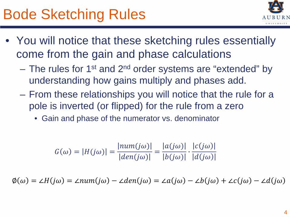
• You will notice that these sketching rules essentially come from the gain and phase calculations– The rules for 1st and 2nd order systems are “extended” by

understanding how gains multiply and phases add.– From these relationships you will notice that the rule for a

pole is inverted (or flipped) for the rule from a zero• Gain and phase of the numerator vs. denominator

𝐺𝐺 𝜔𝜔 = 𝐻𝐻(𝑗𝑗𝜔𝜔) =𝑛𝑛𝑛𝑛𝑛𝑛(𝑗𝑗𝜔𝜔)𝑑𝑑𝑑𝑑𝑛𝑛(𝑗𝑗𝜔𝜔)

=𝑎𝑎(𝑗𝑗𝜔𝜔)𝑏𝑏(𝑗𝑗𝜔𝜔)

𝑐𝑐 𝑗𝑗𝜔𝜔𝑑𝑑 𝑗𝑗𝜔𝜔

4

∅ 𝜔𝜔 = ∠𝐻𝐻 𝑗𝑗𝜔𝜔 = ∠𝑛𝑛𝑛𝑛𝑛𝑛 𝑗𝑗𝜔𝜔 − ∠𝑑𝑑𝑑𝑑𝑛𝑛 𝑗𝑗𝜔𝜔 = ∠𝑎𝑎 𝑗𝑗𝜔𝜔 − ∠𝑏𝑏 𝑗𝑗𝜔𝜔 + ∠𝑐𝑐 𝑗𝑗𝜔𝜔 − ∠𝑑𝑑 𝑗𝑗𝜔𝜔

Bode Sketching Rules

• Draw your vertical and horizontal axis– Label horizontal axis ω (rad/s)– Label the top vertical axis Gain– Label the bottom vertical axis Phase (or φ)

• Mark the magnitude of all zeros and poles on the frequency axis– It is sometimes helpful to draw the poles and zeros

on the s-plane (or at least calculate their magnitudes and damping ratios if they are under-damped)

5

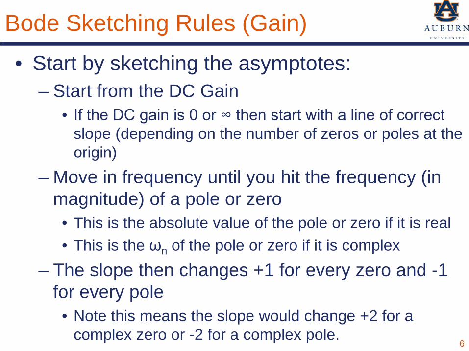
Bode Sketching Rules (Gain)• Start by sketching the asymptotes:

– Start from the DC Gain• If the DC gain is 0 or ∞ then start with a line of correct

slope (depending on the number of zeros or poles at the origin)

– Move in frequency until you hit the frequency (in magnitude) of a pole or zero

• This is the absolute value of the pole or zero if it is real• This is the ωn of the pole or zero if it is complex

– The slope then changes +1 for every zero and -1 for every pole

• Note this means the slope would change +2 for a complex zero or -2 for a complex pole.

6

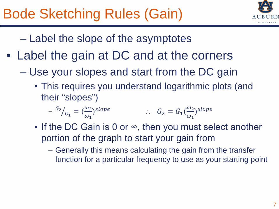
Bode Sketching Rules (Gain)– Label the slope of the asymptotes

• Label the gain at DC and at the corners– Use your slopes and start from the DC gain

• This requires you understand logarithmic plots (and their “slopes”)

– 𝐺𝐺2𝐺𝐺1 = (𝜔𝜔2

𝜔𝜔1)𝑠𝑠𝑠𝑠𝑜𝑜𝑜𝑜𝑠𝑠 ∴ 𝐺𝐺2 = 𝐺𝐺1(𝜔𝜔2

𝜔𝜔1)𝑠𝑠𝑠𝑠𝑜𝑜𝑜𝑜𝑠𝑠

• If the DC Gain is 0 or ∞, then you must select another portion of the graph to start your gain from

– Generally this means calculating the gain from the transfer function for a particular frequency to use as your starting point

7

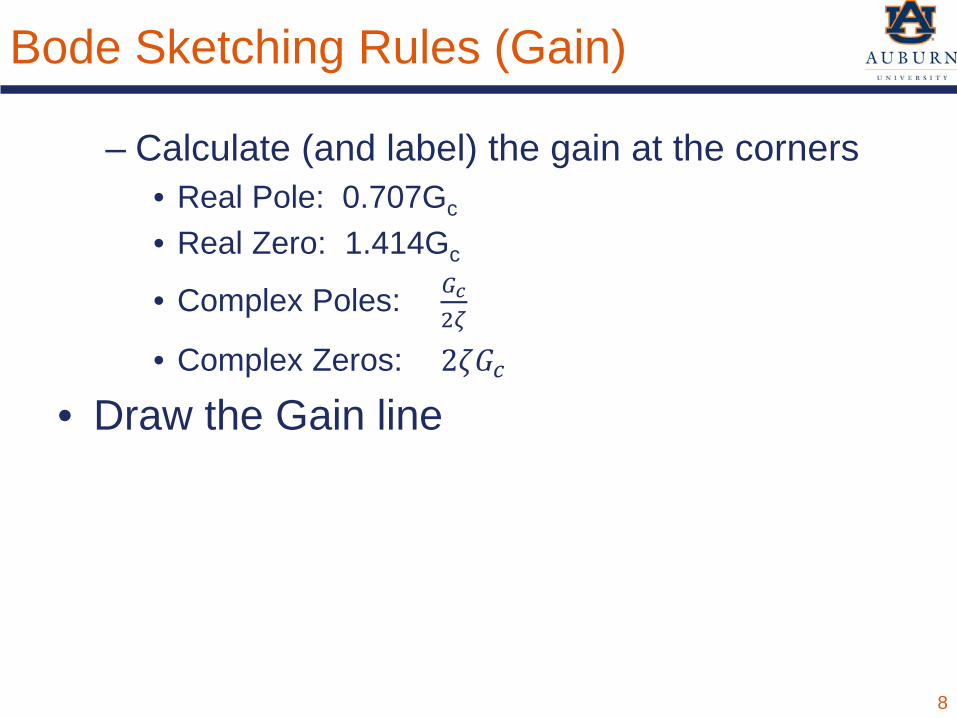
Bode Sketching Rules (Gain)

– Calculate (and label) the gain at the corners• Real Pole: 0.707Gc

• Real Zero: 1.414Gc

• Complex Poles: 𝐺𝐺𝑐𝑐2𝜁𝜁

• Complex Zeros: 2𝜁𝜁𝐺𝐺𝑐𝑐• Draw the Gain line

8

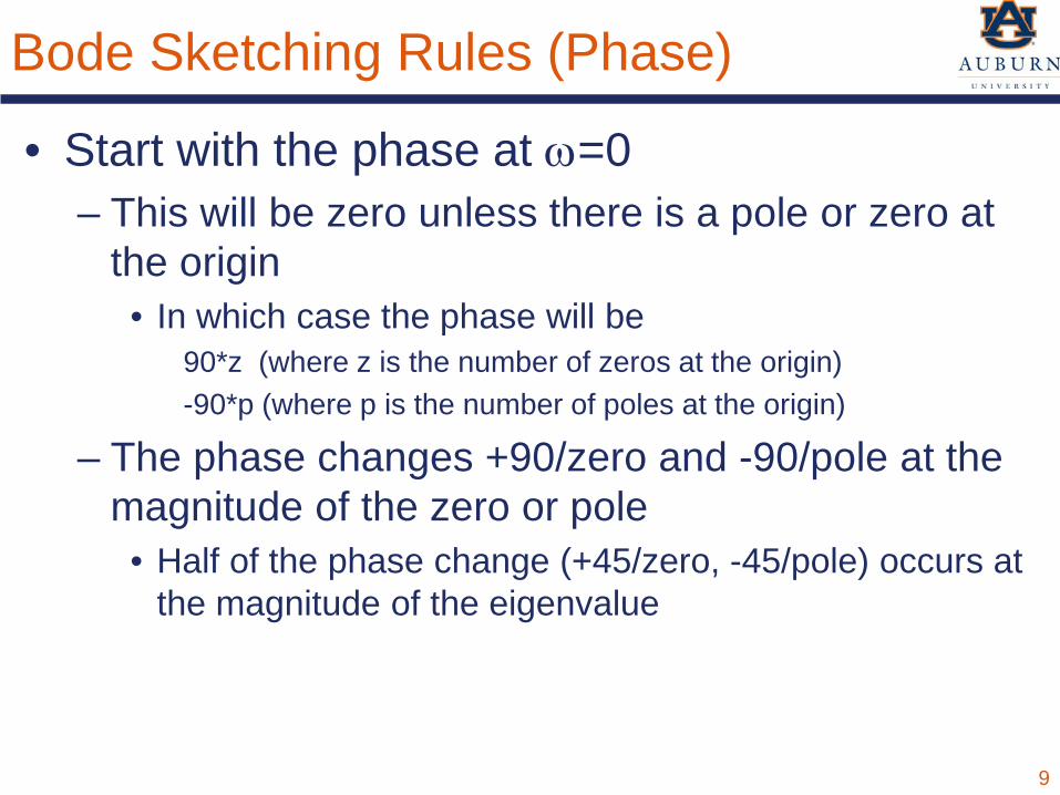
Bode Sketching Rules (Phase)

• Start with the phase at ω=0– This will be zero unless there is a pole or zero at

the origin• In which case the phase will be

90*z (where z is the number of zeros at the origin)-90*p (where p is the number of poles at the origin)

– The phase changes +90/zero and -90/pole at the magnitude of the zero or pole

• Half of the phase change (+45/zero, -45/pole) occurs at the magnitude of the eigenvalue

9

Comments

• Note that these sketching rules produce very rough ideas for the bode plot (or the frequency response)– But the provide insight into design and

analysis.

10

Maxon DC16 Spec Sheet

https://www.maxongroup.com/medias/sys_master/root/8833376059422/19-EN-94.pdf 11

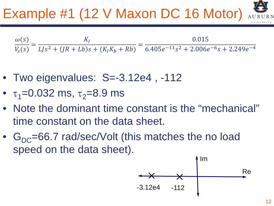
Example #1 (12 V Maxon DC 16 Motor)𝜔𝜔(𝑠𝑠)𝑉𝑉𝑠𝑠(𝑠𝑠)

=𝐾𝐾𝐼𝐼

𝐿𝐿𝐿𝐿𝑠𝑠2 + 𝐿𝐿𝐽𝐽 + 𝐿𝐿𝑏𝑏 𝑠𝑠 + (𝐾𝐾𝐼𝐼𝐾𝐾𝑏𝑏 + 𝐽𝐽𝑏𝑏)=

0.0156.405𝑑𝑑−11𝑠𝑠2 + 2.006𝑑𝑑−6𝑠𝑠 + 2.249𝑑𝑑−4

• Two eigenvalues: S=-3.12e4 , -112• τ1=0.032 ms, τ2=8.9 ms• Note the dominant time constant is the “mechanical”

time constant on the data sheet.• GDC=66.7 rad/sec/Volt (this matches the no load

speed on the data sheet).

12

Im

Re

-112-3.12e4

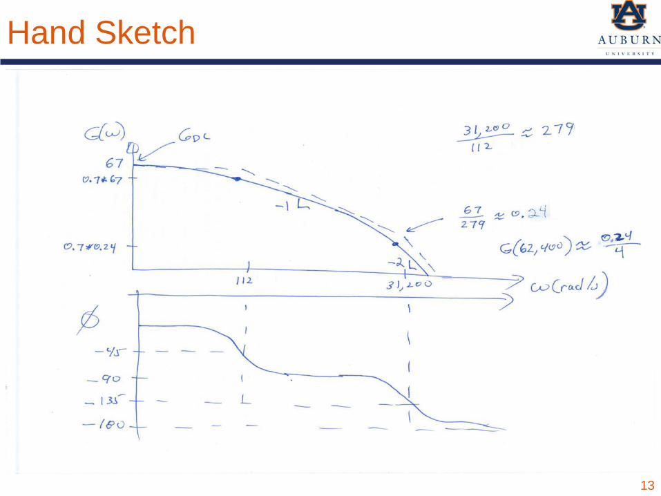
Hand Sketch

13

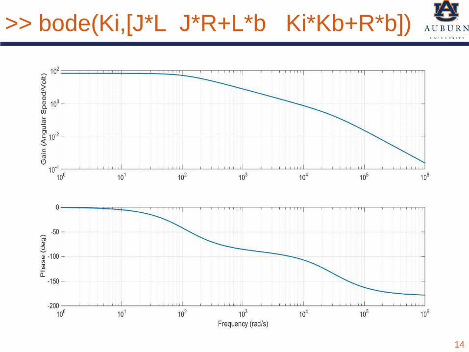
>> bode(Ki,[J*L J*R+L*b Ki*Kb+R*b])

14

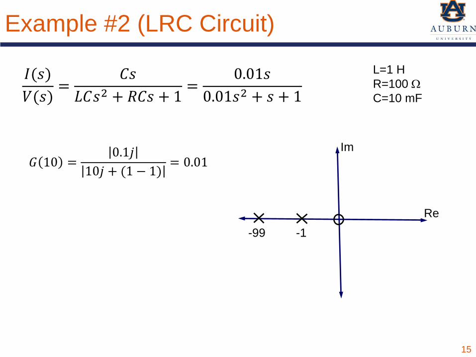
Example #2 (LRC Circuit)

15

L=1 HR=100 ΩC=10 mF

Im

Re-1-99

𝐼𝐼(𝑠𝑠)𝑉𝑉(𝑠𝑠)

=𝐶𝐶𝑠𝑠

𝐿𝐿𝐶𝐶𝑠𝑠2 + 𝐽𝐽𝐶𝐶𝑠𝑠 + 1=

0.01𝑠𝑠0.01𝑠𝑠2 + 𝑠𝑠 + 1

𝐺𝐺 10 =0.1𝑗𝑗

10𝑗𝑗 + (1 − 1)= 0.01

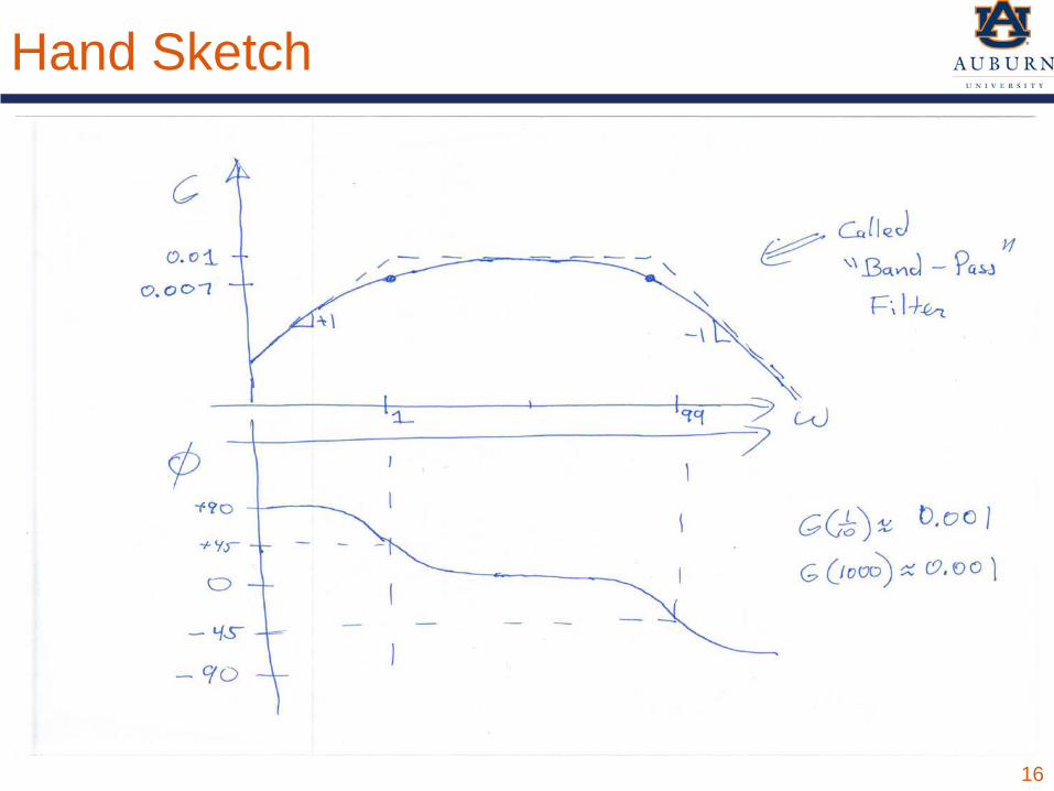
Hand Sketch

16

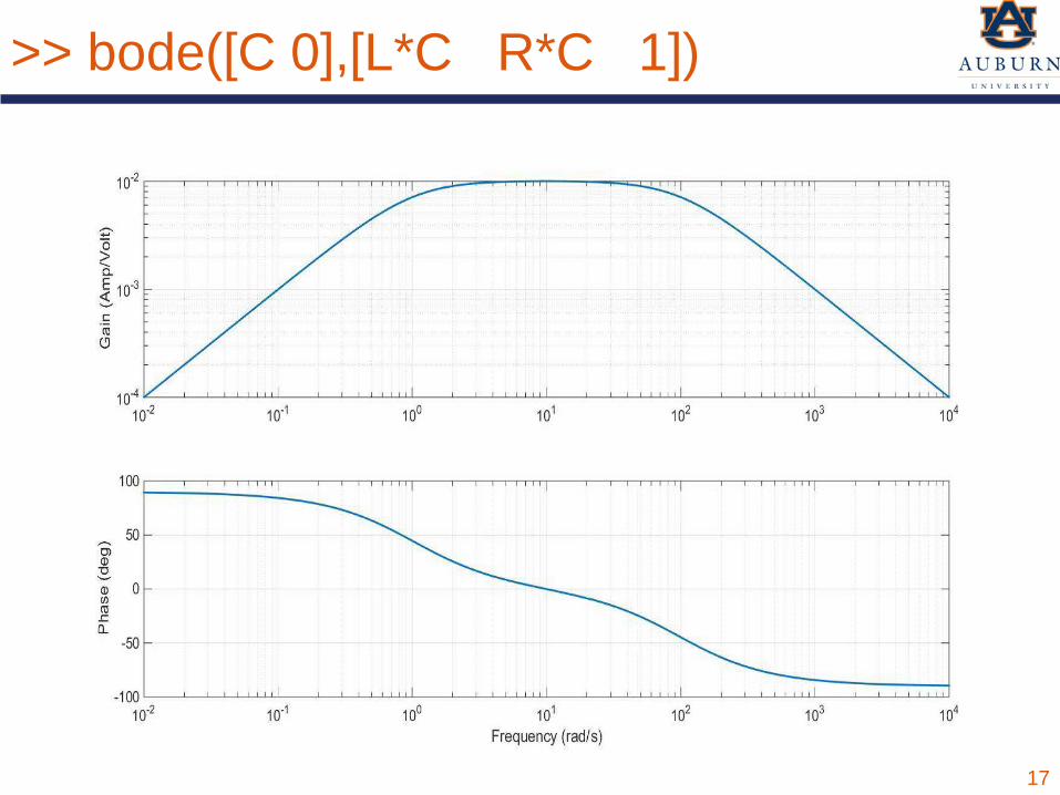
>> bode([C 0],[L*C R*C 1])

17

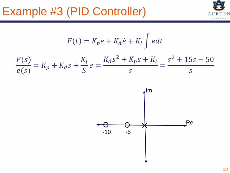
Example #3 (PID Controller)

𝐹𝐹 𝑡𝑡 = 𝐾𝐾𝑜𝑜𝑑𝑑 + 𝐾𝐾𝑑𝑑𝑑 + 𝐾𝐾𝐼𝐼 𝑑𝑑𝑑𝑑𝑡𝑡

𝐹𝐹(𝑠𝑠)𝑑𝑑(𝑠𝑠)

= 𝐾𝐾𝑜𝑜 + 𝐾𝐾𝑑𝑑𝑠𝑠 +𝐾𝐾𝐼𝐼𝑆𝑆𝑑𝑑 =

𝐾𝐾𝑑𝑑𝑠𝑠2 + 𝐾𝐾𝑜𝑜𝑠𝑠 + 𝐾𝐾𝐼𝐼𝑠𝑠

=𝑠𝑠2 + 15𝑠𝑠 + 50

𝑠𝑠

18

Im

Re-5-10

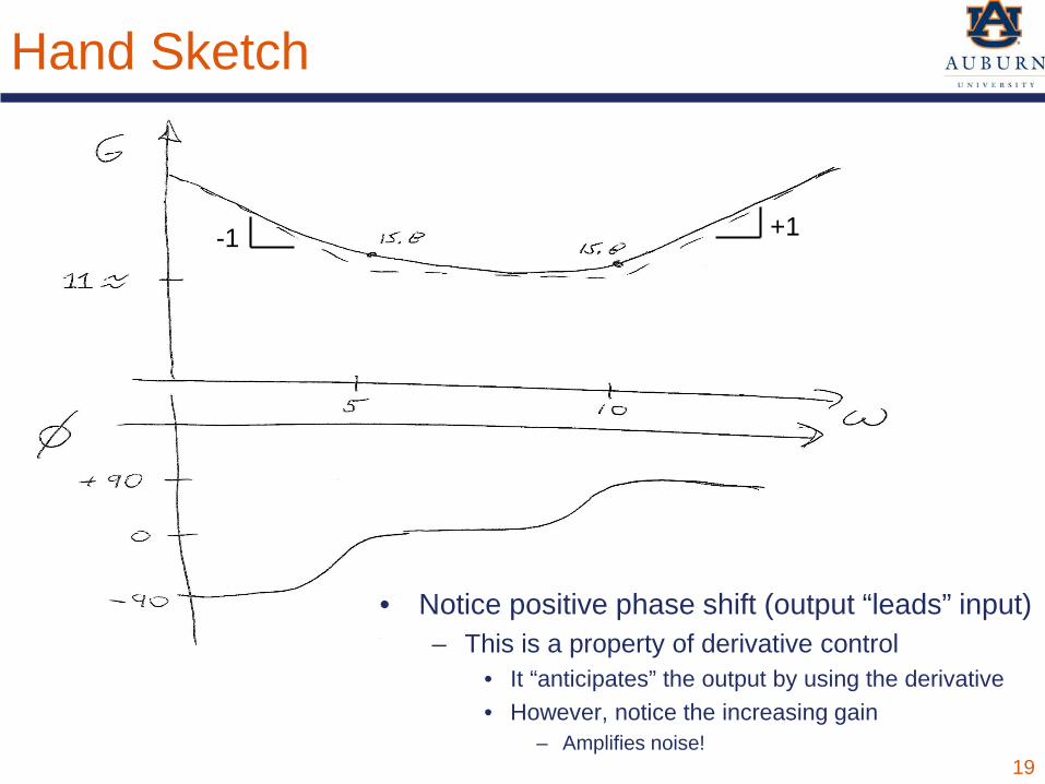
Hand Sketch

19

• Notice positive phase shift (output “leads” input)– This is a property of derivative control

• It “anticipates” the output by using the derivative• However, notice the increasing gain

– Amplifies noise!

-1 +1

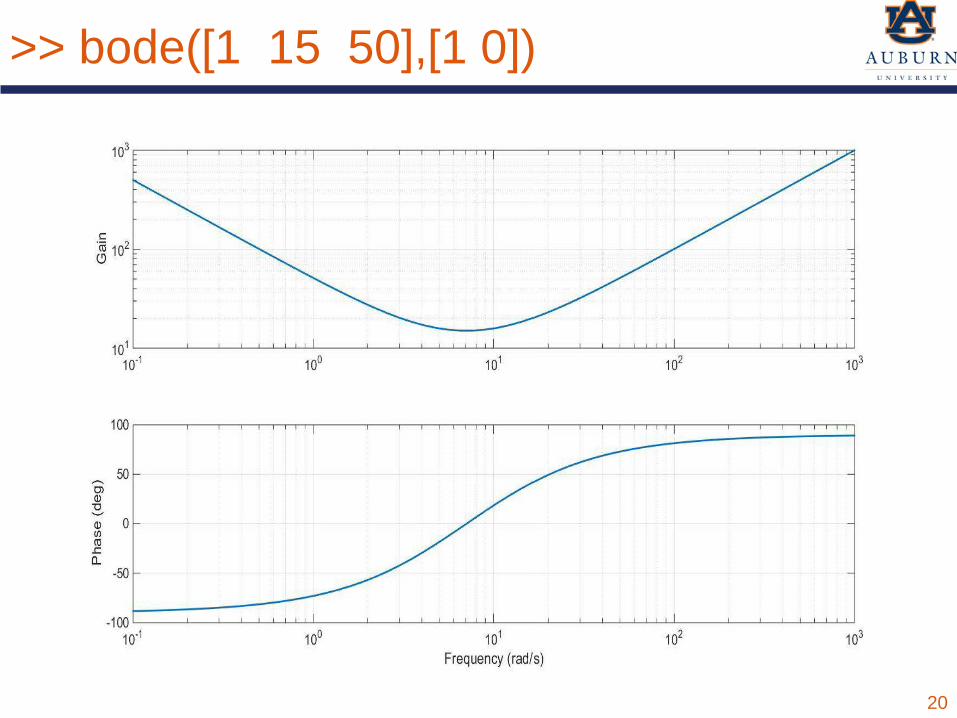
>> bode([1 15 50],[1 0])

20

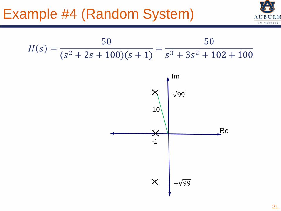
Example #4 (Random System)

𝐻𝐻 𝑠𝑠 =50

(𝑠𝑠2 + 2𝑠𝑠 + 100)(𝑠𝑠 + 1)=

50𝑠𝑠3 + 3𝑠𝑠2 + 102 + 100

21

Im

Re-1

10

99

− 99

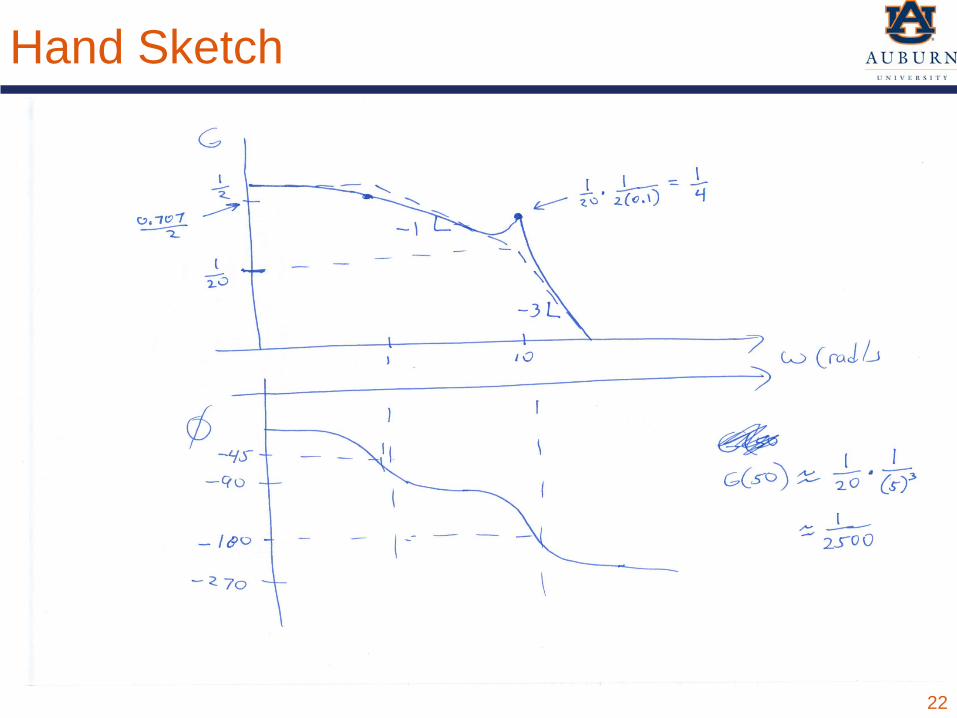
Hand Sketch

22

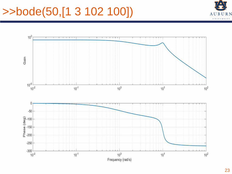
>>bode(50,[1 3 102 100])

23

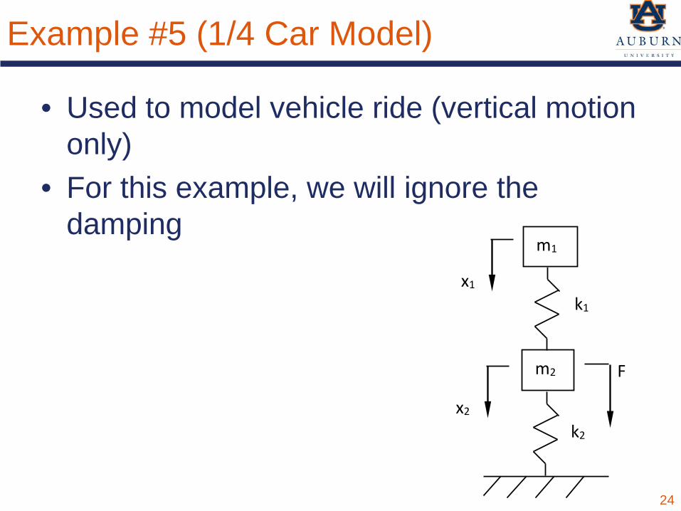
Example #5 (1/4 Car Model)

• Used to model vehicle ride (vertical motion only)

• For this example, we will ignore the damping

24

m2 F

k2

m1

k1

x2

x1

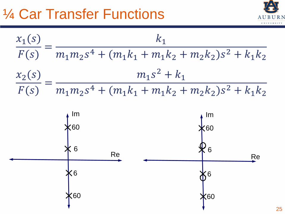
¼ Car Transfer Functions𝑥𝑥1(𝑠𝑠)𝐹𝐹(𝑠𝑠)

=𝑘𝑘1

𝑛𝑛1𝑛𝑛2𝑠𝑠4 + (𝑛𝑛1𝑘𝑘1 + 𝑛𝑛1𝑘𝑘2 + 𝑛𝑛2𝑘𝑘2)𝑠𝑠2 + 𝑘𝑘1𝑘𝑘2𝑥𝑥2(𝑠𝑠)𝐹𝐹(𝑠𝑠)

=𝑛𝑛1𝑠𝑠2 + 𝑘𝑘1

𝑛𝑛1𝑛𝑛2𝑠𝑠4 + (𝑛𝑛1𝑘𝑘1 + 𝑛𝑛1𝑘𝑘2 + 𝑛𝑛2𝑘𝑘2)𝑠𝑠2 + 𝑘𝑘1𝑘𝑘2

25

Im

Re

6

60

60

6

Im

Re

6

60

60

6

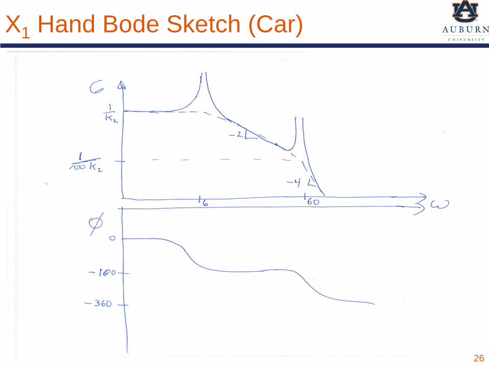
X1 Hand Bode Sketch (Car)

26

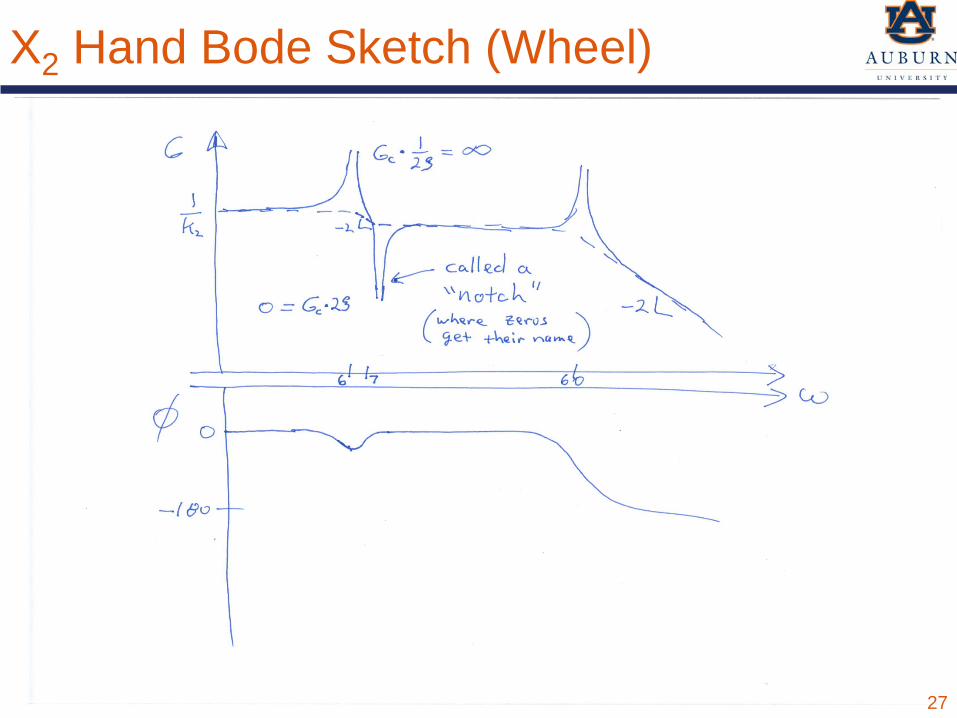
X2 Hand Bode Sketch (Wheel)

27

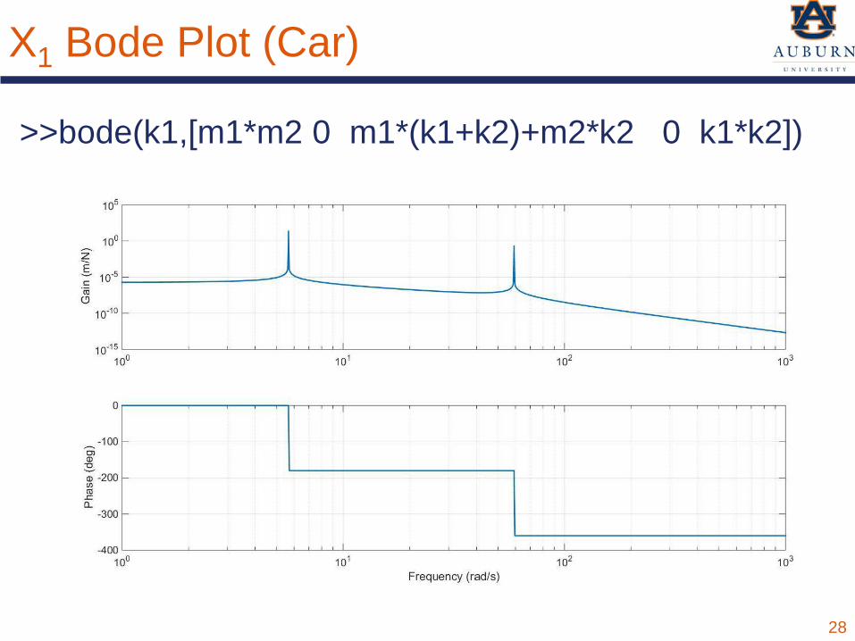
X1 Bode Plot (Car)

28

>>bode(k1,[m1*m2 0 m1*(k1+k2)+m2*k2 0 k1*k2])

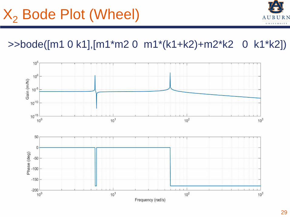
X2 Bode Plot (Wheel)

>>bode([m1 0 k1],[m1*m2 0 m1*(k1+k2)+m2*k2 0 k1*k2])

29

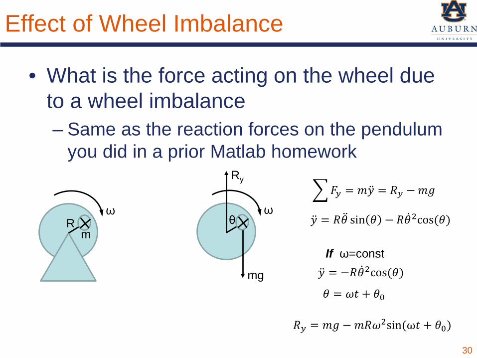
Effect of Wheel Imbalance

• What is the force acting on the wheel due to a wheel imbalance– Same as the reaction forces on the pendulum

you did in a prior Matlab homework

30

Rω

m

ω

mg

Ry𝐹𝐹𝑦𝑦 = 𝑛𝑛𝑦 = 𝐽𝐽𝑦𝑦 −𝑛𝑛𝑚𝑚

𝑦 = 𝐽𝐽𝜃 sin 𝜃𝜃 − 𝐽𝐽𝜃2cos(𝜃𝜃)θ

𝑦 = −𝐽𝐽𝜃2cos(𝜃𝜃)If ω=const

𝜃𝜃 = 𝜔𝜔𝑡𝑡 + 𝜃𝜃0

𝐽𝐽𝑦𝑦 = 𝑛𝑛𝑚𝑚 −𝑛𝑛𝐽𝐽𝜔𝜔2sin(ω𝑡𝑡 + 𝜃𝜃0)

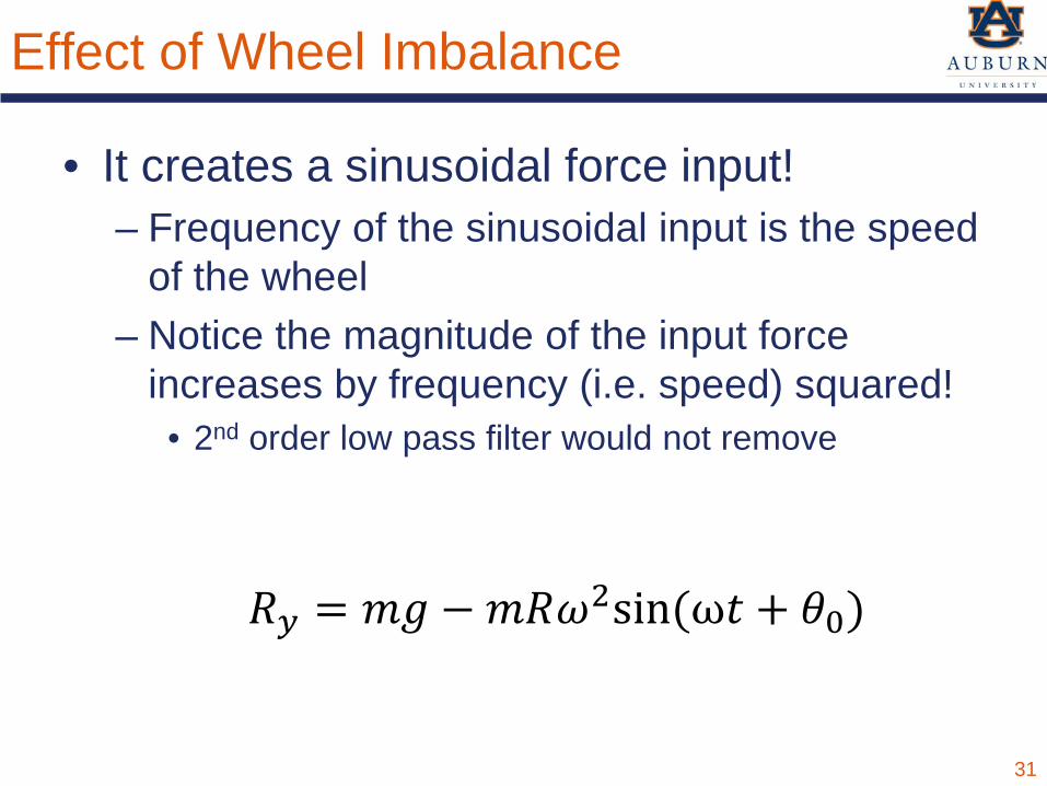
Effect of Wheel Imbalance

• It creates a sinusoidal force input!– Frequency of the sinusoidal input is the speed

of the wheel– Notice the magnitude of the input force

increases by frequency (i.e. speed) squared!• 2nd order low pass filter would not remove

31

𝐽𝐽𝑦𝑦 = 𝑛𝑛𝑚𝑚 −𝑛𝑛𝐽𝐽𝜔𝜔2sin(ω𝑡𝑡 + 𝜃𝜃0)

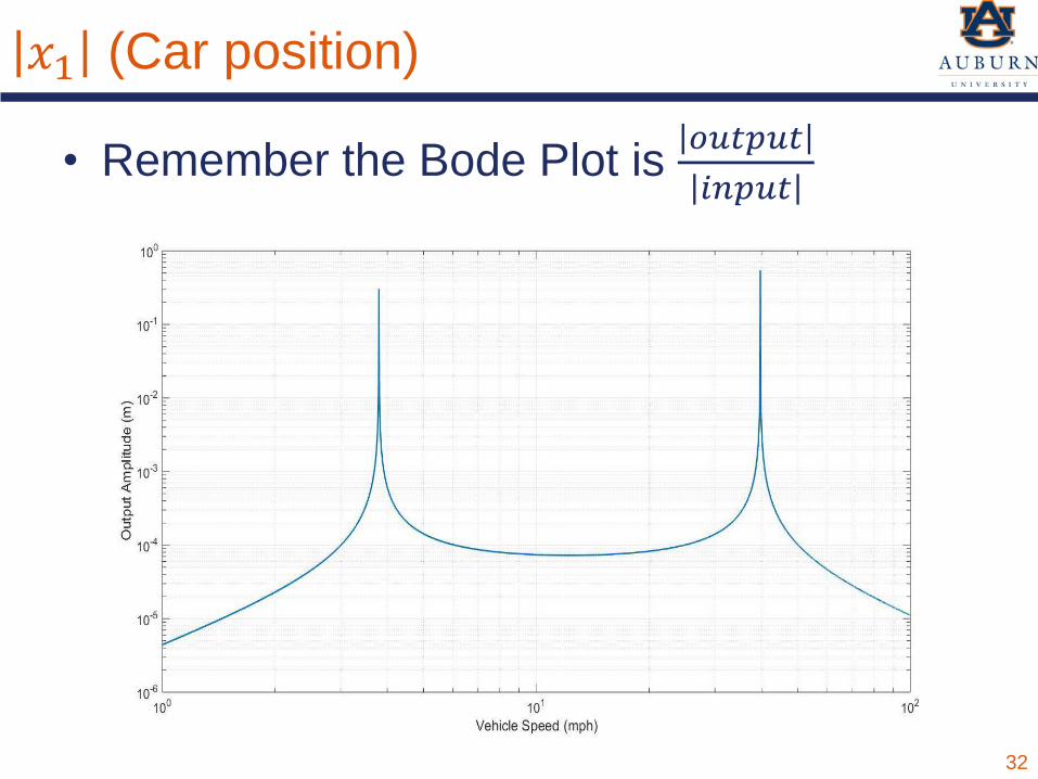
𝑥𝑥1 (Car position)

• Remember the Bode Plot is 𝑜𝑜𝑜𝑜𝑜𝑜𝑜𝑜𝑜𝑜𝑜𝑜𝑖𝑖𝑖𝑖𝑜𝑜𝑜𝑜𝑜𝑜

32

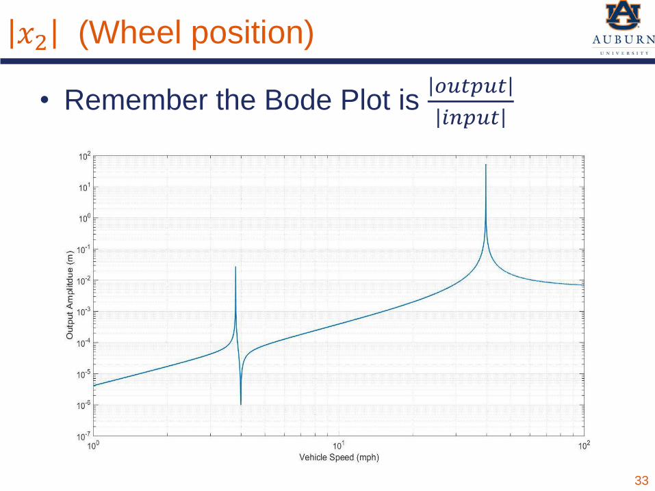
𝑥𝑥2 (Wheel position)

• Remember the Bode Plot is 𝑜𝑜𝑜𝑜𝑜𝑜𝑜𝑜𝑜𝑜𝑜𝑜𝑖𝑖𝑖𝑖𝑜𝑜𝑜𝑜𝑜𝑜

33

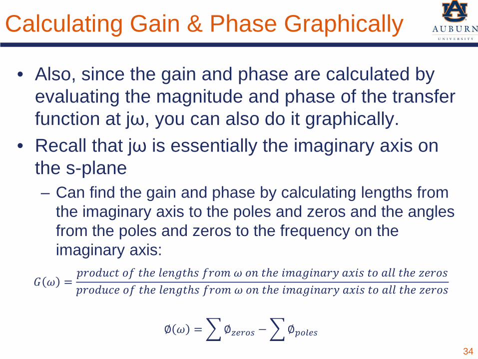
Calculating Gain & Phase Graphically

• Also, since the gain and phase are calculated by evaluating the magnitude and phase of the transfer function at jω, you can also do it graphically.

• Recall that jω is essentially the imaginary axis on the s-plane– Can find the gain and phase by calculating lengths from

the imaginary axis to the poles and zeros and the angles from the poles and zeros to the frequency on the imaginary axis:

𝐺𝐺 𝜔𝜔 =𝑝𝑝𝑝𝑝𝑝𝑝𝑑𝑑𝑛𝑛𝑐𝑐𝑡𝑡 𝑝𝑝𝑜𝑜 𝑡𝑡𝑡𝑑𝑑 𝑙𝑙𝑑𝑑𝑛𝑛𝑚𝑚𝑡𝑡𝑡𝑠𝑠 𝑜𝑜𝑝𝑝𝑝𝑝𝑛𝑛 𝜔𝜔 𝑝𝑝𝑛𝑛 𝑡𝑡𝑡𝑑𝑑 𝑖𝑖𝑛𝑛𝑎𝑎𝑚𝑚𝑖𝑖𝑛𝑛𝑎𝑎𝑝𝑝𝑦𝑦 𝑎𝑎𝑥𝑥𝑖𝑖𝑠𝑠 𝑡𝑡𝑝𝑝 𝑎𝑎𝑙𝑙𝑙𝑙 𝑡𝑡𝑡𝑑𝑑 𝑧𝑧𝑑𝑑𝑝𝑝𝑝𝑝𝑠𝑠𝑝𝑝𝑝𝑝𝑝𝑝𝑑𝑑𝑛𝑛𝑐𝑐𝑑𝑑 𝑝𝑝𝑜𝑜 𝑡𝑡𝑡𝑑𝑑 𝑙𝑙𝑑𝑑𝑛𝑛𝑚𝑚𝑡𝑡𝑡𝑠𝑠 𝑜𝑜𝑝𝑝𝑝𝑝𝑛𝑛 𝜔𝜔 𝑝𝑝𝑛𝑛 𝑡𝑡𝑡𝑑𝑑 𝑖𝑖𝑛𝑛𝑎𝑎𝑚𝑚𝑖𝑖𝑛𝑛𝑎𝑎𝑝𝑝𝑦𝑦 𝑎𝑎𝑥𝑥𝑖𝑖𝑠𝑠 𝑡𝑡𝑝𝑝 𝑎𝑎𝑙𝑙𝑙𝑙 𝑡𝑡𝑡𝑑𝑑 𝑧𝑧𝑑𝑑𝑝𝑝𝑝𝑝𝑠𝑠

∅ 𝜔𝜔 = ∅𝑧𝑧𝑠𝑠𝑧𝑧𝑜𝑜𝑠𝑠 −∅𝑜𝑜𝑜𝑜𝑠𝑠𝑠𝑠𝑠𝑠34

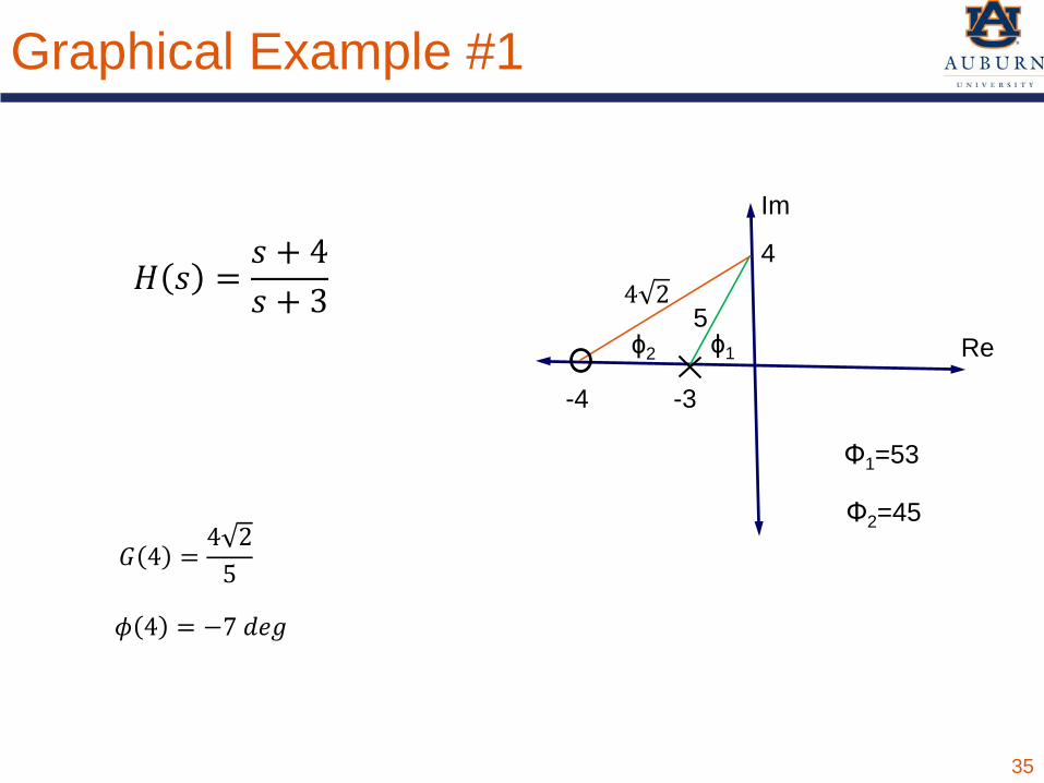
Graphical Example #1

35

4

Im

Re

𝐻𝐻 𝑠𝑠 =𝑠𝑠 + 4𝑠𝑠 + 3

-3-4

54 2

ϕ1ϕ2

𝐺𝐺 4 =4 2

5

𝜙𝜙 4 = −7 𝑑𝑑𝑑𝑑𝑚𝑚

Φ1=53

Φ2=45

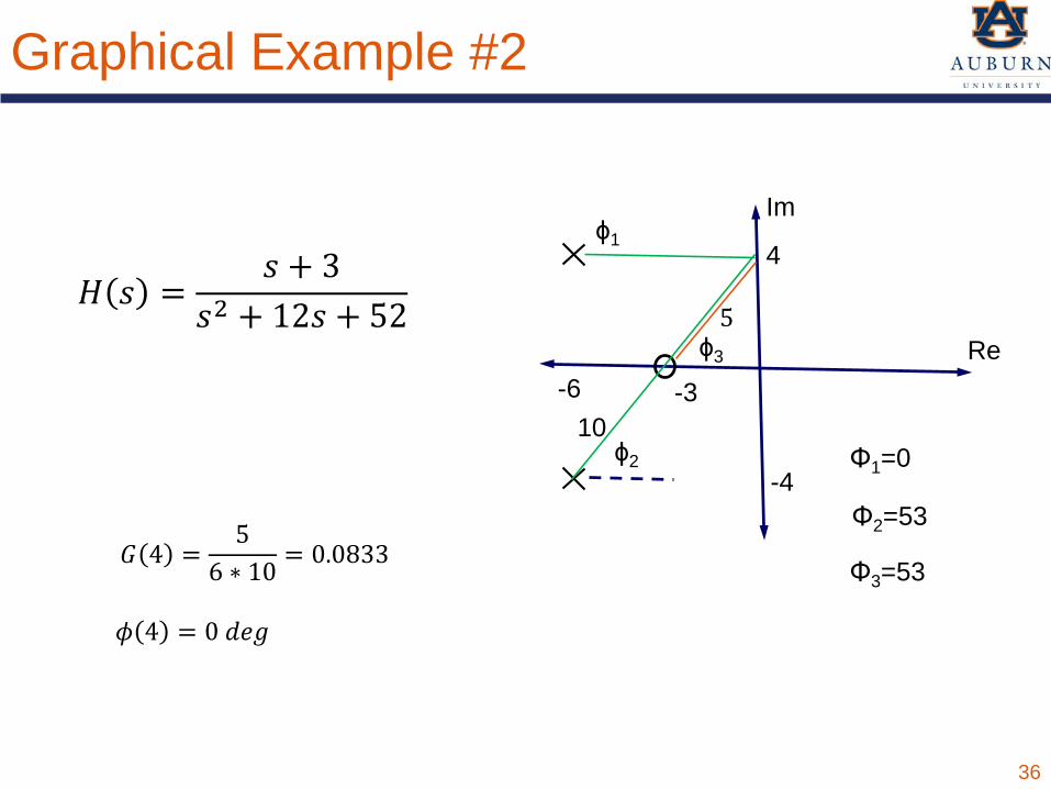
Graphical Example #2

36

4

Im

Re

𝐻𝐻 𝑠𝑠 =𝑠𝑠 + 3

𝑠𝑠2 + 12𝑠𝑠 + 52

-6 -310

5

ϕ1

ϕ3

𝐺𝐺 4 =5

6 ∗ 10 = 0.0833

𝜙𝜙 4 = 0 𝑑𝑑𝑑𝑑𝑚𝑚

Φ1=0

Φ2=53

ϕ2-4

Φ3=53