AnalyticNumberTheory - Imperial College Londondcheragh/Teaching/2016-S-ANT/ANT.pdf · formula for...
66
Analytic Number Theory Davoud Cheraghi May 13, 2016 Contents 1 Introduction 2 2 Arithmetic Functions 6 3 Dirichlet Series 18 4 Analytic Properties of the Riemann Zeta-Function 26 5 The Proof of the Prime Number Theorem 37 6 Further Properties of ζ (s) 54 7 References 66
Transcript of AnalyticNumberTheory - Imperial College Londondcheragh/Teaching/2016-S-ANT/ANT.pdf · formula for...
Analytic Number Theory
Davoud Cheraghi
May 13, 2016
Contents
1 Introduction 2
2 Arithmetic Functions 6
3 Dirichlet Series 18
4 Analytic Properties of the Riemann Zeta-Function 26
5 The Proof of the Prime Number Theorem 37
6 Further Properties of ζ(s) 54
7 References 66
1 Introduction
The fundamental questions in number theory concern the interplay between the additive and
multiplicative structures on the integers. An example of a typical theorem from number
theory is:
Theorem. (Lagrange’s Theorem) Every n ∈ N is a sum of 4 squares
n =
4∑
i=1
n2i ,
where ni ∈ Z.
The proof of the above theorem “works in” Z.
This course is an introduction to analytic number theory. That is, we turn to techniques
from analysis, where we apply continuous methods to study discrete phenomena. Often these
are statements involving approximations. In analytic number theory we often ask roughly
how frequent are integers with a certain property P . For instance, one cannot give an exact
formula for the number of primes in an interval [1, x], but we can establish an asymptotic
formula, and give some upper bounds for the discrepancy between the exact and asymptotic
formulas. Although this methodology turns out to be unexpectedly powerful, we must remain
humble. It is easy to pose simple looking open (and probably extremely hard) questions about
prime numbers, including:
• (Twin primes problem) Are there infinitely many pairs of consecutive primes which
differ by 2?
• (Sophie Germain problem) Are there infinitely many pairs of primes p, q such that
q = 2p+ 1?
• (Goldbach problem) Is every even integer n > 2 equal to the sum of two primes?
There are also many number theoretic statements where it is not obvious that analytic
methods are appropriate. Example of theorems whose proofs use analysis are the following
1. Every integer is a sum of at most
(a) 4 squares,
2
(b) 9 cubes,
(c) 19 fourth powers,
(d) 37 fifth powers, etc.
This was proved, by the combined efforts of many mathematicians, in 1986. It answers
a question of Waring dating from 1770.
2. The sequence of primes contains arbitrarily long arithmetic progressions. eg: 7, 37, 67,
97, 127, 157 is a progression of 6 primes. This was proved in 2004.
3. The ring{
a+ b√14 : a, b ∈ Z
}
= Z[√14] is a Euclidean domain.
4. Every odd number n ≥ 7 is a sum of 3 primes. (Proved in 2013). Goldbach’s conjecture
(still undecided) was that every even number n ≥ 4 is a sum of 2 primes and every odd
number n ≥ 7 is a sum of 3 primes.
In this course our use of analysis will mainly involve the theory of complex functions,
specifically the notions of analytic (holomorphic) and meromorphic functions. One can argue
that one is really using properties of real harmonic functions, since the real and imaginary
parts of a holomorphic function have that property. There are instances where one gets
number-theoretic information by considering harmonic functions in a setting where there is
no complex structure.
This course is primarily concerned with arithmetic functions and prime numbers. We
make the following definition.
Definition 1.1. π(x) = # {p ≤ x : p prime}.
The key question we shall examine is: How fast does π(x) grow? The first result on this
question was proved by Euclid:
Theorem 1.2. π(x) → ∞ as x→ ∞.
Numerical results suggest that π(x) is roughly x/ log x. The primes appear to thin out
the higher one goes, so that for numbers up to x, about one number out of log x is prime.
This conjecture is due to Gauss and dates from 1849.
3
Let us define
Li(x) =
ˆ x
2
dt
log t.
In problem sheet one you will show that
limx→∞
x/ log x
Li(x)= 1.
The fundamental result, verifying Gauss’ conjecture is:
Theorem 1.3. (The Prime Number Theorem – Hadamard, de la Vallee Poussin 1896)
limx→∞
π(x)
x/ log x= 1
or equivalently
limx→∞
π(x)
Li(x)= 1.
It is convenient to introduce some notation.
Definition 1.4. If f, g : [1,∞) → R with g(x) > 0 for all x, we say that f(x) ∼ g(x) iff(x)g(x) → 1 as x→ ∞.
Hence the PNT (Prime Number Theorem) states that π(x) ∼ xlog x ∼ Li(x).
Definition 1.5. Let f, g : [1,∞) → R be functions with g(x) > 0, for all x. We say that
f(x) = O(g(x)) if |f(x)/g(x)| is bounded from above, that is, if there exists a constant c > 0
such that for all x we have |f(x)| ≤ cg(x).
In particular, a relation of the form f(x) = g(x) +O(h(x)) for real functions f , g, and h
defined on (0,∞) means that |f(x)− g(x)| = O(h(x).
Example. We have sinx = O(1) and sinx = O(x). Observe that, with the O(·) notation,
equality is no longer symmetric (!) Note also the fact that f(x) = O(g(x)) does not imply
that f ′(x) = O(g′(x)).
Tables reveal that the detailed distribution of primes is very erratic. There are a lot of
pairs of primes which differ by 2, such as (11, 13), (17, 19), (29, 31), etc. It is a famous open
problem however whether there are infinitely many such “prime-twins”.
4
There are arbitrarily large gaps among the primes. Consider the numbers N ! + 2, N ! +
3, . . . , N ! +N . These are all composite, since if k ≤ N then k | N ! + k.
Open problem: Roughly how large is the largest gap between consecutive primes up to
N? A plausible conjecture is that the largest gap is ∼ (logN)2.
For all x ≥ 20 for which π(x) has been calculated one finds that
x
log x< π(x) < Li(x).
The first inequality has in fact been proved to hold for x ≥ 20. As to the second inequality,
there are good reasons to suppose π(x) < Li(x) for all x ≤ 10100. However Littlewood showed
in 1912 that π(x)− Li(x) changes sign infinitely often, and it is now known that there exists
an x ≤ 10316 such that π(x) > Li(x). This is a remarkable result. In every case that π(x)
has ever been calculated, comprising billions of data points, one has π(x) < Li(x). However
we know that the inequality eventually fails: In mathematics “experimental evidence” is not
good enough – only proper proof will do!
5
2 Arithmetic Functions
We denote the set of positive integers with N.
Definition. An arithmetic function is a mapping f : N → C.
Definition. A multiplicative arithmetic function is one for which f(mn) = f(m)f(n), when-
ever (m,n) = 1.
One might imagine that it would be more natural to define a multiplicative function to
be one satisfying f(mn) = f(m)f(n) for all m,n. However, this condition is too restrictive.
Example. We define the unit function u : N → C as u(n) = 1 for all n. This is a multiplicative
arithmetic function. Similarly uc(n) = nc, where c ∈ R is fixed, is multiplicative.
The function ω(n) = # {p | n : p prime} is not multiplicative, since, for example ω(2) =
1, ω(3) = 1 but ω(6) = 2 6= 1× 1.
Other important arithmetic functions are:-
– d(n) = # {k ∈ N : k | n}. This is called the divisor function.
– σ(n) =∑
k|n k,
– φ(n) = # {k ∈ N : k ≤ n, (k, n) = 1} = #(Z/nZ)× = # {k + nZ : (k, n) = 1}. This is
called the Euler function.
The notations ω(n), d(n), σ(n) and φ(n) are standard; but u(n) and uc(n) were invented for
these notes!
An obvious fact is that if f, g are multiplicative, then so is (fg)(n) = f(n)g(n).
Definition. The Dirichlet convolution of f and g is defined as
(f ∗ g)(n) =∑
ab=n;a,b∈Nf(a)g(b).
For example,
(d ∗ ω)(6) = d(1)ω(6) + d(2)ω(3) + d(3)ω(2) + d(6)ω(1)
= 1× 2 + 2× 1 + 2× 1 + 4× 0 = 6.
Note also the following facts
6
1. (u ∗ u)(n) =∑ab=n u(a)u(b) =∑
ab=n 1 = d(n). Hence u ∗ u = d.
2. (u ∗ u1)(n) =∑
ab=n u(a)u1(b) =∑
ab=n b =∑
b|n b = σ(n). Hence, u ∗ u1 = σ.
Theorem 2.1. If F and G are multiplicative, then so is F ∗G.
Corollary 2.2. The functions d(n) and σ(n) are multiplicative.
Lemma 2.3. Suppose that (m,n) = 1. Then every pair a, b ∈ N with ab = mn, takes the
form a = cd and b = ef with ce = m, df = n; and this expression is unique.
Proof
First we prove the existence of c, d, e, f . Take
c = (a,m), d = a/c, e = (b,m), f = b/e.
It follows that c, d, e, f ∈ N. So it remains to show that ce = m, df = n. We will show that
(a,m)(b,m) = m (⋆). It will follow that ce = m, and that df = ab/ce = mn/ce = n as
required.
To show (⋆), we use repeatedly the fact that (α, β)γ = (αγ, βγ). This yields
(a,m)(b,m) = (a(b,m),m(b,m))
= ((ab, am),m(b,m))
= ((mn, am),m(b,m))
= (m(n, a),m(b,m))
= m((n, a), (b,m)).
However (n, a) | n and (b,m) | m and we know that (m,n) = 1. Hence ((n, a), (b,m)) = 1,
and so the expression above reduces to m.
It remains to prove uniqueness. Suppose a = c′d′ and b = e′f ′, with c′e′ = m and d′f ′ = n.
Then, since (m,n) = 1, we have (e′, d′) = 1. Hence
c = (a,m) = (c′d′, c′e′) = c′(d′, e′) = c′.
Similarly, d = d′ and so e = e′ and f = f ′.
Proof (Of Theorem 2.1)
7
Take (m,n) = 1. We have to show that (F ∗G)(m)(F ∗G)(n) = (F ∗G)(mn).
LHS =
{
∑
m=ce
F (c)G(e)
}
∑
df=n
F (d)G(f)
=∑
c,d,e,f∈Nce=m,df=n
F (c)F (d)G(e)G(f).
However, c | m and d | n where (m,n) = 1. Hence (c, d) = 1. This gives F (c)F (d) = F (cd).
Similarly for (e, f) = 1. Hence
LHS =∑
ce=m,df=n
F (cd)G(ef)
and by Lemma 2.3, each pair a, b for which ab = mn, arises just once as a = cd and b = ef .
Thus
LHS =∑
ab=mn
F (a)G(b) = (F ∗G)(mn).
Theorem 2.4. If f(n) is multiplicative and n = pe11 · · · pekk , where pi are distinct primes, then
f(n) =∏ki=1 f(p
eii ).
Corollary 2.5. We have d(pe11 · · · pekk ) = (e1 + 1) · · · (ek + 1).
Proof d(peii ) = # {1, pi, . . . , peii } = ei + 1.
Corollary 2.6.
σ(pe11 · · · pekk ) =
k∏
i=1
pei+1i − 1
pi − 1.
Proof σ(peii ) = 1 + pi + . . . + peii =pei+1
i −1pi−1 .
Proof (Of Theorem 2.4)
We work by induction on k. For k = 1 we have f(pe11 ) = f(pe11 ). In general,
f(pe11 · · · pekk ) = f(pe11 · · · pek−1
k−1 )f(pekk )
8
since (pe11 . . . pek−1
k−1 , pekk ) = 1. The induction hypothesis then yields
k−1∏
i=1
f(peii )f(pekk )
which produces the required result.
Corollary 2.7. If f, g are multiplicative then f = g if and only if f(pe) = g(pe) for all prime
powers pe.
As an example of a typical question we can now answer, we ask how large is d(n)? Clearly
d(p) = 2 for all primes p, but sometimes d(n) is large.
Theorem 2.8. For all k ∈ N one has d(n) ≥ (log n)k for infinitely many n.
Proof
Let p1, . . . , pk+1 be the first k +1 primes. Set n = (p1 · · · pk+1)m. We claim that if m is large
enough, then d(n) ≥ (log n)k.
We have
d(n) = (m+ 1)k+1 > mk+1 =
(
log n
log p1 · · · pk+1
)k+1
and this exceeds (log n)k providing that log n > (log p1 · · · pk+1)k+1. It therefore suffices to
take m > (log p1 · · · pk+1)k.
Theorem 2.9. For every ǫ > 0 there exists a constant cǫ such that d(n) ≤ cǫnǫ for all n ∈ N.
Remark. This result can be re-phrased as saying that d(n) = O(nǫ) for all ǫ > 0.
Proof
We have d(n) ≤ n, so we can take cǫ = 1 for all ǫ ≥ 1. Thus we may now assume that ǫ < 1.
For n = pe11 · · · perr we have
d(n)
nǫ=∏ 1 + ei
pǫeii.
Then, for primes pi with pi ≥ 21/ǫ we have
1 + eipǫeii
≤ 1 + ei2ei
≤ 1,
9
since 2m ≥ 1 +m for all m ∈ N. For the remaining primes, for which 2 ≤ pi < 21/ǫ, we have
pǫeii ≥ 2ǫei = eǫei log 2 ≥ 1 + ǫei log 2 > ǫ log 2 + ǫei log 2 = ǫ(log 2)(1 + ei).
Hence,
1 + eipǫeii
≤
1 for pi ≥ 21/ǫ,
1ǫ log 2 for pi < 21/ǫ.
Hence, with pi ranging through the various prime factors of n, we have
d(n)
nǫ≤
∏
pi<21/ǫ
(
1
ǫ log 2
)
.
Thus, if p ranges over all primes less than 21/ǫ, whether or not they divide n, we have
d(n)
nǫ≤
∏
p<21/ǫ
(
1
ǫ log 2
)
.
Denote the product on the right by cǫ, and note that this does not depend on n. Thend(n)nǫ ≤ cǫ for all n, as required.
We may also ask how large is d(n) on average?
Theorem 2.10. We have
limN→∞
∑
n≤N d(n)∑
n≤N log n= 1.
Equivalently,∑
n≤N d(n) ∼∑
n≤N log n. More precisely,
∑
n≤Nd(n) = N logN +O(N),
∑
n≤Nlog n = N logN +O(N).
So d(n) is, on average, of size log n
10
Lemma 2.11. If f : [1,∞) → [0,∞) is increasing, then
ˆ N
1f(x)dx ≤
N∑
1
f(n) ≤ f(N) +
ˆ N
1f(x)dx
while if f is decreasing, then
ˆ N
1f(x)dx ≤
N∑
1
f(n) ≤ f(1) +
ˆ N
1f(x)dx.
Proof
If f is increasing
ˆ n
n−1f(x)dx ≤ f(n) ≤
ˆ n+1
nf(x)dx
and so
N∑
1
f(n) ≥ f(1) +N∑
n=2
ˆ n
n−1f(x)dx = f(1) +
ˆ N
1f(x)dx ≥
ˆ N
1f(x)dx
and
N∑
1
f(n) ≤ f(N) +N−1∑
n=1
ˆ n+1
nf(x)dx = f(N) +
ˆ N
1f(x)dx.
The decreasing case is similar.
Corollary 2.12. We have
logN ≤N∑
n=1
1
n≤ 1 + logN,
N logN −N ≤N∑
n=1
log n ≤ N logN.
Proof
Apply Lemma 2.11 with f(x) = 1/x (the decreasing case), and the first statement follows.
11
For f(x) = log x (the increasing case), we haveˆ N
1f(x)dx =
ˆ N
1log x dx = N logN −N + 1
so
N logN −N ≤ N logN −N + 1 =
ˆ N
1f(x)dx ≤
N∑
1
log n
and
N∑
1
log n ≤N∑
1
logN = N logN.
We now prove Theorem 2.10
Proof
We have∑
n≤Nd(n) =
∑
n=ab≤N1 =
∑
a,bab≤N
1 =∑
a≤N#
{
b : b ≤ N
a
}
.
For θ ∈ R set [θ] = max {k ∈ Z : k ≤ θ}. Then if θ ≥ 0 one sees that # {b ∈ N : b ≤ θ} =
[θ].
For example, [π] = 3 and {b ∈ N : b ≤ π} = {1, 2, 3}. Hence∑
n≤Nd(n) =
∑
a≤N
[
N
a
]
.
However, for all θ ∈ R we have [θ] = θ +O(1), and so [N/a] = N/a+O(1). This produces
∑
a≤N
[
N
a
]
=∑
a≤N
(
N
a+O(1)
)
=∑
a≤N
N
a+O(N) = N
∑
a≤N
1
a+O(N)
which in turn is N{logN+O(1)}+O(N), by Corollary 2.12. Finally, this is N logN+O(N)+
O(N), and so
∑
a≤N
[
N
a
]
= N logN +O(N).
We now introduce another important arithmetic function.
12
Definition. (The Mobius Function)
Set µ(1) = 1 and
µ(pe11 · · · pekk ) =
(−1)k if ei = 1 for all i,
0 if ei ≥ 2 for some i,
where pi are distinct primes.
Note that µ(n) is a multiplicative function. This follows directly from the definition, but
may take a moment’s thought.
The following result gives the key property for the Mobius function.
Theorem 2.13. We have
(µ ∗ u)(n) =∑
d|nµ(d) =
1 if n = 1,
0 if n ≥ 2.
Proof
Set f = µ ∗ u. Then f is multiplicative, by Theorem 2.1, since µ, u are multiplicative. Now if
e ≥ 1 then
f(pe) =∑
ab=pe
µ(a)u(b) =∑
a|peµ(a)
= µ(1) + µ(p) + . . .+ µ(pe) = 1 + (−1) + 0 + . . .+ 0 = 0.
Hence, in general, f(pe11 · · · pekk ) = 0 if any exponent is greater than or equal to 1. The case
where n = 1 is trivial.
Remark. Set
I(n) =
1 if n = 1,
0 if n ≥ 2.
This function is trivially multiplicative. The result above tells us that µ ∗ u = I. Note also
that
(I ∗ f)(n) =∑
ab=n
I(a)f(b) = I(1)f(n) = f(n)
for all f . Hence, I ∗ f = f .
13
Theorem 2.14. Let M = {f : N → C : f(1) = 1} and
M0 = {f ∈M : fmultiplicative} .
Then (M, ∗) is an abelian group with identity I, and M0 is a subgroup.
Proof
It is trivial that f ∗ g = g ∗ f , that I ∗ f = f , and also that M is closed under the ∗ operation.
For associativity we note that
(f ∗ (g ∗ h))(n) =∑
ab=n
f(a)(g ∗ h)(b)
=∑
ab=n
f(a)∑
cd=b
g(c)h(d)
=∑
a,c,dacd=n
f(a)g(c)h(d),
which is clearly independent of the ordering and the bracketing of f, g, h. This proves as-
sociativity. In the last step of the above we used the fact that there exists a one-to-one
correspondence between
{
(a, b, c, d) ∈ N4 : ab = n, b = cd}
and{
(a, c, d) ∈ N3 : n = acd}
via the maps (a, b, c, d) 7→ (a, c, d) and (a, c, d) 7→ (a, cd, c, d).
The existence of inverses requires a little more work. Given f ∈ M , define g inductively
by setting g(1) = 1 and then, if g(1), . . . , g(n − 1) have been defined, putting
g(n) := −∑
a,bab=n, b<n
f(a)g(b).
Then
(f ∗ g)(n) =∑
ab=nb<n
f(a)g(b) + f(1)g(n) =∑
ab=nb<n
f(a)g(b) + g(n) = 0
if n ≥ 2. Trivially, (f ∗ g)(1) = f(1)g(1) = 1. It follows that f ∗ g = I, which completes the
proof that M is a group.
14
As for M0, we know that f, g ∈M0 means that f, g are multiplicative. Hence f ∗ g is also
multiplicative, whence f ∗ g ∈ M0. It remains to prove that if f is multiplicative, then so is
f−1.
We proceed to define a function h on prime powers. Let h(1) = 1, and inductively set
h(pe) = −∑
0≤k<eh(pk)f(pe−k).
We then define h on the whole of N by setting h(pe11 · · · perr ) = h(pe11 ) · · · h(perr ). Thus h is
automatically multiplicative. We claim that f ∗h = I. It will follow that f−1 is multiplicative,
since f−1 = h.
To prove that f ∗ h = I we note that f and h are multiplicative, whence f ∗ h is too. The
function I is multiplicative. It is therefore sufficient to show that f ∗h agrees with I for every
prime power pe. To do so, we note that
(f ∗ h)(p0) = f(1)h(1) = 1 = I(p0).
Moreover, for e ≥ 1 we have
(f ∗ h)(pe) =∑
0≤k≤eh(pk)f(pe−k)
=∑
0≤k<eh(pk)f(pe−k) + h(pe)f(1)
=∑
0≤k<eh(pk)f(pe−k) + h(pe)
= 0 = I(pe).
This is sufficient to show that f ∗ h = I, which completes the proof.
Theorem 2.15. (The Mobius Inversion Formula) Given arithmetic functions f, g, we have
that
∑
d|ng(d) = f(n) ∀n⇔ g(n) =
∑
d|nf(d)µ
(n
d
)
∀n.
15
Proof
We have
∑
d|ng(d) = f(n) ⇔
∑
de=n
g(d)u(e) = f(n) ⇔ g ∗ u = f.
Similarly
g(n) =∑
d|nf(d)µ(n/d) ⇔ g(n) =
∑
de=n
f(d)µ(e) ⇔ g = f ∗ µ.
Hence the theorem is equivalent to the claim that g ∗ u = f ⇔ g = f ∗ µ. But g ∗ u =
f ⇒ (g ∗ u) ∗ µ = f ∗ µ ⇒ g ∗ (u ∗ µ) = f ∗ µ ⇒ g ∗ I = f ∗ µ ⇒ g = f ∗ µ. Similarly,
f ∗ µ = g ⇒ (f ∗ µ) ∗ u = g ∗ u⇒ f ∗ (µ ∗ u) = g ∗ u⇒ f = g ∗ u.
We now examine the function φ(n) = # {k : k ≤ n, (k, n) = 1}.
Theorem 2.16. We have φ ∗ u = u1, or equivalently∑
d|n φ(d) = n.
Proof
Let n be given. We partition {1, 2, . . . , n} into disjoint subsets according to the highest com-
mon factor which each element has with n. This produces sets Ad = {k ∈ N : k ≤ n, (k, n) = d}.There is one such set for each d | n.
We claim that #Ad = φ(n/d), from which it will follow that
n =∑
d|n#Ad =
∑
d|nφ(n/d) =
∑
n=de
φ(e) =∑
e|nφ(e)
as required.
To prove the claim we observe that if (k, n) = d then d | k. Set k = dj and n =
de, so that d = (k, n) = (dj, de) = d(j, e). It follows that (j, e) = 1. Thus, #Ad =
# {dj : dj ≤ de, (j, e) = 1} = # {j : j ≤ e, (j, e) = 1} = φ(e), as required.
Corollary 2.17. We have φ = µ ∗ u1, so that φ(n) =∑
d|n µ(d)nd = n
∑
d|nµ(d)d .
Proof
The result follows from Theorem 2.16, by the Mobius inversion formula, Theorem 2.15. Specif-
ically, we have φ = φ ∗ I = φ ∗ (u ∗ µ) = (φ ∗ u) ∗ µ = u1 ∗ µ.
16
Corollary 2.18. The function φ is multiplicative.
Proof
The functions µ and u1 are multiplicative, and hence their convolution is also multiplicative.
Corollary 2.19.
φ(pe11 · · · pekk ) =
k∏
i=1
pei−1i (pi − 1)
and
φ(n) = n∏
p|n(1− 1
p).
Proof
We have
φ(pe) = # {n : n ≤ pe, (n, pe) = 1} = # {n : n ≤ pe, p ∤ n}
= # {n : n ≤ pe} −# {n : n ≤ pe, p | n} = pe − pe−1 = pe(1− 1/p).
17
3 Dirichlet Series
We recall the Euler’s viewpoint on the fact, originally due to Euclid, that there are infinitely
many prime numbers. Euclids original proof was quite simple, and entirely algebraic: assume
there are only finitely many primes, multiply them together, add 1, then factor the result.
Euler realized instead that a basic fact from analysis also leads to the infinitude of primes.
This fact is the divergence of the harmonic series
1 +1
2+
1
3+
1
4+ . . . .
On the other hand, if there were only finitely many primes, then unique factorization of
positive integers into prime powers would imply that
∞∑
n=1
1
n=∏
p
(
1 +1
p+
1
p2+ . . .
)
=∏
p
(
1− 1
p
)−1.
This would give the equality between a divergent series and a finite quantity. Euler’s idea
turns out to be quite fruitful: the introduction of analysis into the study of prime numbers
allows us to prove distribution statements about primes in a much more flexible fashion than
is allowed by algebraic techniques.
A Dirichlet series is a series of the form
F (s) =
∞∑
n=1
f(n)n−s
where f(n) is an arithmetic function, and s ∈ C.
It is conventional, for historical reasons, to use s as a complex variable in this setting, and
to write it as a sum of real and imaginary parts as s = σ+ it. Since s is complex we must be
careful to specify what we mean by n−s. We define it as n−s = e−s logn where the branch of
the logarithm function is chosen so that log n is real.
The series above may converge for all s, as in the example∑∞
n=1 e−nn−s, or it may diverge
for all s, as shown by the series∑∞
n=1 enn−s. However in many cases there are some values
where the series converges and others where it diverges.
Theorem 3.1. Suppose that there exists an s1 such that F (s1) is absolutely convergent, and
an s2 such that F (s2) is not absolutely convergent. Define
S = {Re(s) : F (s) is absolutely convergent} .
18
We then have that
1. The set S has an infimum, σ0 say.
2. F (s) is absolutely convergent for all s with Re(s) > σ0.
3. If η > 0 then F (s) is uniformly convergent on {s : Re(s) ≥ σ0 + η}.
4. F (s) is holomorphic on {s : Re(s) > σ0} with derivatives
F (k)(s) = (−1)k∞∑
n=1
f(n)(log n)kn−s.
5. The series for F (k)(s) is absolutely convergent for Re(s) > σ0.
Remark. The number σ0 is known as the “abscissa of absolute convergence” for the series∑
f(n)n−s, which we will abbreviate as AAC.
Before we embark on proving the above theorem we recall a basic result from complex
analysis.
Lemma 3.2. Let U be an open subset of C and let F1(z), . . . , Fn(z), . . . be holomorphic on
U . Suppose∑
n Fn(z) is uniformly convergent on U to F (z). Then F (z) is holomorphic on
U , with F (k)(z) =∑
n F(k)n (z).
Proof
See the complex analysis course.
Proof (Of Theorem 3.1)
1) Suppose that Re(s) < Re(s2). Then
∑∣
∣f(n)n−s∣
∣ ≥∑
∣
∣f(n)n−s2∣
∣ = ∞.
Thus Re(s) /∈ S, whence S is bounded below by Re(s2). Moreover S is non-empty, since
Re(s1) ∈ S. Thus S is non-empty and bounded below, and hence has an infimum.
2) If Re(s) > σ0 then by the definition of an infimum, there exists an s3 such that
Re(s3) ≤ Re(s) and∑ |f(n)n−s3 | < ∞. It follows that
∑ |f(n)n−s| < ∞ by the comparison
test, since |f(n)n−s| ≤ |f(n)n−s3| for Re(s) ≥ Re(s3).
19
3) Recall the Weierstrass M -test. This states that if one has sequences of functions fn(z)
and of real numbers Mn, such that |fn(z)| ≤ Mn for all z in some region D, then∑∞
1 fn(z)
converges uniformly on D providing that∑∞
1 Mn converges.
We apply this to the functions fn(s) = f(n)n−s and the region {s : Re(s) ≥ σ0 + η}. We
take Mn = |f(n)|n−σ0−η, so that we do indeed have the required condition |f(n)n−s| ≤ Mn.
We know from part 2 that∑
Mn converges, since σ0 + η > σ0. The result of part 3 then
follows from the M -test.
4) Suppose that Re(s) = σ > σ0. Define η = (σ − σ0)/2 and U = {z : Re(z) > σ0 + η}.By part 3 of the theorem the sum for F (z) is uniformly convergent on U . Thus, by Lemma
3.2 (below) we deduce that F (s) is holomorphic at s, with
F (k)(s) =
∞∑
n=1
(
d
ds
)k(
f(n)n−s)
= (−1)k∞∑
n=1
f(n)(log n)kn−s.
5) Let σ0 < σ∗ < Re(s). Then∑ |f(n)n−σ∗ | is absolutely convergent by part 2 of the
theorem. Moreover∣
∣
∣
∣
(log n)kn−s
n−σ∗
∣
∣
∣
∣
= (log n)kn−(Re(s)−σ∗) → 0.
Hence, by the comparison test, the series for F (k)(s) is absolutely convergent.
Remark. One may also define an “abscissa of conditional convergence” by
σ1 = inf {Re(s) : F (s) is convergent} .
One always has σ1 ≤ σ0, but in some cases σ1 is strictly less than σ0. However we always
have σ0− 1 ≤ σ1 ≤ σ0. One can show that the series for F (s) is convergent for all s such that
Re(s) > σ1 and F (s) is holomorphic for Re(s) > σ1. (See problem sheet 2).
We now relate all this to the Dirichlet convolution.
Theorem 3.3. Let f1(n) and f2(n) be arithmetic functions and define f3 = f1 ∗ f2. Assume
that the Dirichlet series F1(s) =∑
n f1(n)n−s and F2(s) =
∑
n f2(n)n−s have abscissae
of absolute convergence equal to σ1, σ2 respectively. Then F3(s) =∑
n f3(n)n−s converges
absolutely for σ > max(σ1, σ2) and F3(s) = F1(s)F2(s).
20
Proof
If σ > max(σ1, σ2) then∑
f1(n)n−s and
∑
f2(n)n−s are absolutely convergent. We may
therefore multiply them together and rearrange the terms at will, and the result will still be
absolutely convergent.
It follows that
F1(s)F2(s) =∞∑
n1=1
∞∑
n2=1
f1(n1)f2(n2)n−s1 n−s2
=
∞∑
n=1
[
∑
n1n2=n
f1(n1)f2(n2)
]
n−s
=∞∑
n=1
(f1 ∗ f2)(n)n−s
=
∞∑
n=1
f3(n)n−s,
as required.
Theorem 3.4. Suppose that f(n) is a multiplicative function and suppose that F (s) =∑
n f(n)n−s has AAC equal to σ0. Then
F (s) =∏
p prime
{ ∞∑
e=0
f(pe)p−es}
for σ > σ0, in the sense that the sums Fp(s) =∑∞
e=0 f(pe)p−es have AAC less than or equal
to σ0, and
F (s) = limx→∞
∏
p≤xFp(s)
for σ > σ0.
Proof
The sum∑∞
e=0 f(pe)p−es contains a subset of the terms in
∑∞1 f(n)n−s and so has AAC at
most σ0. Let p1, . . . , pk be the primes less than or equal to x. Then
∏
p≤xFp(s) =
∏
j≤k
{ ∞∑
e=0
f(pej)p−esj
}
.
21
When σ > σ0 this is a finite product of absolutely convergent series. It is therefore permissible
to multiply out the product and rearrange the terms freely. We therefore produce
∞∑
n=1
n−s
∑
n=pe11
···pekk
f(pe11 · · · , pekk )
.
We shall write θx(n) for the number of different ways that n can be written as a prod-
uct pe11 · · · pekk . The unique factorisation property for N tells us that θx(n) = 0 or 1; and
θx(n) = 1 for n ≤ x. Moreover, because f is multiplicative, we have f(n) = f(pe11 · · · pekk ) =
f(pe11 ) · · · f(pekk ). It follows that
∏
p≤xFp(s) =
∞∑
n=1
n−sf(n)θx(n).
We may therefore conclude that
∣
∣
∣
∣
∣
∣
F (s)−∏
p≤xFp(s)
∣
∣
∣
∣
∣
∣
=
∣
∣
∣
∣
∣
∞∑
n=1
n−sf(n)(1− θx(n))
∣
∣
∣
∣
∣
≤∞∑
n=1
n−σ |f(n)| (1− θx(n)) ( since∣
∣n−s∣
∣ = n−σ)
≤∑
n>x
n−σ |f(n)| .
However, since∑∞
1 n−σ |f(n)| converges we know that
limx→∞
∑
n>x
n−σ |f(n)| = 0.
It follows that
limx→∞
∣
∣
∣
∣
∣
∣
F (s)−∏
p≤xFp(s)
∣
∣
∣
∣
∣
∣
= 0
as required.
Definition. An arithmetic function fn is said to be totally multiplicative if f(mn) = f(m)f(n)
for all m and n in N.
22
Corollary 3.5. If f(n) is totally multiplicative then, under the conditions of Theorem 3.4 we
have
F (s) =∏
p prime
1
1− f(p)ps
for σ > σ0.
Proof
Fp(s) =
∞∑
e=0
f(pe)p−es =∞∑
e=0
f(p)ep−es
=1
1− f(p)p−s.
Definition. The Riemann Zeta-function is given by the series
ζ(s) =∞∑
n=1
n−s
which has AAC= 1.
According to the above corollary we then have
ζ(s) =∞∑
n=1
1
ns=
∏
p prime
1
1− 1ps.
This important relation is known as the Euler product.
Remark. The Euler product identity for ζ(s) is the key to the importance of the zeta-function.
It is, in effect, an analytic statement of the Fundamental Theorem of Arithmetic. It relates
the additive structure of the integers, through the infinite sum, to the multiplicative structure,
given by the product. The fact that the primes appear in the product, but not in the sum,
allows us to use the zeta-function to extract information about the primes.
In order to motivate the next stage of the argument we will argue informally for a moment.
If we could take logarithms we would obtain log ζ(s) =∑
p− log(1−p−s). Differentiating this
23
gives
d
dslog ζ(s) = ζ ′(s)/ζ(s) = −
∑
p
d
dslog(1− p−s)
= −∑
p
p−s log p1− p−s
= −∑
p
∞∑
e=1
p−es log p.
Of course, taking the logarithm of ζ(s) is dangerous, partly because ζ(s) is complex valued,
but mainly because we do not know that ζ(s) is non-zero.
It is convenient to write the final sum above as a Dirichlet series of the form
∞∑
n=1
n−sΛ(n).
We therefore make the following definition
Definition. Define the von Mangold function by setting
Λ(n) =
log p if n = pe for some prime p and integer e ≥ 1,
0 otherwise.
Note that Λ is not a multiplicative function.
Lemma 3.6. We have (Λ ∗ u)(n) = log n for all n ∈ N.
Proof
(Λ ∗ u)(n) =∑
ab=n
Λ(a) =∑
a|nΛ(a) =
∑
pe|n, e≥1
log p.
If n = pe11 · · · pekk , we get terms for
pe = p1, p21, . . . , p
e11 , p2, p
22, . . . , p
e22 , p3, p
23, . . . .
There are e1 such terms corresponding to powers of p1, each of which contributes log p1, and
then e2 terms corresponding to powers of p2, each contributing log p2, and so on. It follows
that (Λ ∗ u)(n) = e1 log p1 + e2 log p2 + . . . = log n.
24
Theorem 3.7. Let F (s) =∑∞
1 Λ(n)n−s. Then F is absolutely convergent for Re(s) = σ > 1
and F (s)ζ(s) = −ζ ′(s).
Proof
We have
∞∑
1
∣
∣Λ(n)n−s∣
∣ ≤∞∑
1
(log n)n−σ = −ζ ′(σ)
which is absolutely convergent for σ > 1 by Theorem 3.1 part 5. By Theorem 3.3 and the
above lemma we have
F (s)ζ(s) =
∞∑
n=1
(Λ ∗ u)(n)n−s =∞∑
n=1
log nn−s = −ζ ′(s).
25
4 Analytic Properties of the Riemann Zeta-Function
Recall that a complex number s is written as σ+it with σ and t real numbers. The arithmetic
method developed in the previous sections provides us with the following property of the Zeta
function.
Theorem 4.1. If Re(s) > 1 then
1
ζ(s)=
∞∑
n=1
µ(n)n−s.
In particular we deduce that ζ(s) 6= 0 for σ > 1, whence
−ζ′(s)ζ(s)
=∞∑
1
Λ(n)n−s.
Proof
The series∑∞
1 µ(n)/ns has AAC at most 1, by comparison with∑∞
1 n−σ. Moreover, u∗µ = I.
Hence, by Theorem 3.3 we have
ζ(s)∞∑
1
µ(n)
ns=
∞∑
1
I(n)
ns= 1
for σ > 1.
To extract useful information about the primes it turns out that we need to use the zeta-
function for values of s with Re(s) < 1. However, our definition ζ(s) =∑
n−s is not helpful
for Re(s) < 1. Here we give a different formulation of the Zeta function that extends the
domain of definition of ζ(s). It also allows us to derive asymptotic estimates on the size of
this important function.
Theorem 4.2. For s ∈ C and n ∈ N define the functions
fn(s) =
ˆ n+1
n
x− n
xs+1dx
and let
ζ∗(s) =s
s− 1− s
∞∑
n=1
fn(s).
Then, for every n ∈ N we have
26
a) each fn(s) is holomorphic on C;
b) for any η > 0,∑∞
n=1 fn(s) is uniformly convergent on {s ∈ C : Re(s) > η};
c) the function ζ∗(s) is meromorphic on the region Re(s) > 0, with the only singularity
being a simple pole at s = 1, with residue 1;
d) for all s with Re(s) > 1 we have ζ∗(s) = ζ(s).
Remark. This theorem defines a function ζ∗(s) on a region σ > 0, which is strictly larger than
the domain of the original function ζ(s). Moreover the two functions agree wherever they are
both defined. We therefore discard our old definition of ζ(s) and use instead the new one,
for ζ∗(s). This process, in which we extend the domain of definition for a function, is called
“analytic continuation”.
Proof
a) We want to show that fn(s) is holomorphic. For this, we can differentiate under the integral
sign
f ′n(s) =ˆ n+1
n(− log x)
x− n
xs+1dx
using standard results on integration theory. The conditions for this are readily checked, since
(− log x) x−nxs+1 is continuous in x and s, and [n + 1, n] is finite.
b) Next we show that∑∞
1 fn(s) converges uniformly for Re(s) > η. For this we use the
Weierstrass M -test. When Re(s) > η we have
|fn(s)| ≤ˆ n+1
n
dx
|xs+1| =ˆ n+1
n
dx
xσ+1≤ˆ n+1
n
dx
nσ+1=
1
nσ+1≤ 1
nη+1.
We therefore set Mn = n−η−1, so that |fn(s)| ≤ Mn for all s in the region Re(s) > η.
Since∑∞
1 Mn =∑
n−1−η < ∞ we may now apply the M -test and deduce that∑∞
1 fn(s) is
uniformly convergent.
c) Let F (s) =∑
n fn(s). Since this is a uniformly convergent sum of holomorphic functions
(for Re(s) > η) we deduce from Lemma 3.2 that F (s) is holomorphic on {s : Re(s) > η}.However η > 0 is arbitrary, so F (s) must be holomorphic on {s : Re(s) > 0}. It follows that
ζ∗(s) is meromorphic for s > 0, with the only singularity a simple pole at s = 1.
27
Recall that the residue of a meromorphic function at some point s0 is equal to the coeffi-
cient of the term 1/(s− s0) in the Laurent series of the function about s0. In particular, since
sF (s) is bounded at s = 1, its Laurent series has no term of the form 1/(s − 1). The only
contribution comes from s/(s− 1) = 1 + 1/(s − 1), so the residue is equal to 1.
d) Finally we show that ζ∗(s) = ζ(s) for Re(s) > 1. We begin by calculating that
fn(s) =
ˆ n+1
n
x
xs+1dx−
ˆ n+1
n
n
xs+1dx
=1
s− 1
{
n−(s−1) − (n+ 1)−(s−1)}
− n
s
{
n−s − (n+ 1)−s}
,
whence
N∑
n=1
fn(s) =1s−1
∑Nn=1
{
n−(s−1) − (n+ 1)−(s−1)}
−1s
∑Nn=1
{
n−(s−1) − n(n+ 1)−s}
.
The first sum cancels as
{
1−(s−1) − 2−(s−1)}
+{
2−(s−1) − 3−(s−1)}
+ · · ·+{
N−(s−1) − (N + 1)−(s−1)}
= 1−(s−1) − (N + 1)−(s−1).
Similarly the second sum is
{
1 · 1−s − 1 · 2−s}
+ {2 · 2−s − 2 · 3−s}+ · · ·+ {N ·N−s −N · (N + 1)−s}
= 1−s + 2−s + · · · +N−s −N(N + 1)−s.
It follows that
N∑
n=1
fn(s) =1
s− 1
{
1− (N + 1)−(s−1)}
−1
s
{
1−s + 2−s + · · ·+N−s −N(N + 1)−s}
.
We therefore deduce that
s
s− 1− s
N∑
1
fn(s) =s
s− 1(N + 1)−(s−1)
+{
1−s + 2−s + · · ·+N−s}−N(N + 1)−s.
28
Up to this point, any s 6= 1 or 0 would be admissible, but we now assume that Re(s) > 1.
Then as N → ∞ we have ss−1(N +1)−(s−1) → 0. Similarly 1−s+ · · ·+N−s →∑∞
1 n−s = ζ(s)
and also −N(N + 1)−s → 0. It then follows that
ζ∗(s) = limN→∞
s
s− 1− s
N∑
1
fn(s) = ζ(s),
as required.
By adapting this proof we can get information on the size of ζ(s) when Re(s) > 0. For
our purposes it turns out to be sufficient to look at the range Re(s) ≥ 1. Notice in particular
that this includes the case Re(s) = 1 where previously we did not even know that ζ(s) was
defined.
Note that for s with Re(s) ≥ 2, |ζ(s)| ≤ |ζ(2)| <∞. Near the line Re(s) = 1 we have the
following estimate.
Theorem 4.3. If 1 ≤ Re(s) ≤ 2 and |t| ≥ 2 then ζ(s) = O(log |t|), and ζ ′(s) = O(log2 |t|).
Remark. Using only the fact that ζ(s) =∑∞
1 n−s, we see that
|ζ(s)| ≤∞∑
n=1
1
nσ= ζ(σ).
This provides a bound for ζ(s), but as σ ↓ 1 the bound tends to infinity, whereas the
theorem gives a uniform bound throughout the range 1 ≤ σ ≤ 2. Of course we have to
exclude values of s too close to s = 1, since ζ(s) is unbounded near s = 1. By requiring that
|t| ≥ 2 we ensure that log |t| is bounded away from zero. Thus the terms involving log |t| inthe O(. . .) notation are always at least a positive constant.
Proof
The argument used for the previous theorem shows that
s
s− 1− s
N∑
1
fn(s) =s
s− 1(N + 1)−(s−1)
+{
1−s + 2−s + . . .+N−s}−N(N + 1)−s,
29
whence, setting M = N + 1 we have
s
s− 1− s
M−1∑
1
fn(s) =s
s− 1M−(s−1) +
M−1∑
1
n−s − (M − 1)M−s,
= M1−s{1 + 1
s− 1}+ {
M∑
1
n−s −M−s} − {M1−s −M−s}
=M s−1
s− 1+
M∑
n=1
n−s.
It then follows that
ζ∗(s) =s
s− 1− s
∞∑
n=1
fn(s)
=M1−s
s− 1+
M∑
1
n−s − s∞∑
M
fn(s).
We can use this formula with any positive integer value ofM , and we shall chooseM = [|t|].This produces
|ζ∗(σ + it)| ≤ 1
|s− 1| +∑
n≤[|t|]n−σ + |s|
∑
n≥[|t|]
1
nσ+1,
since |M1−s| ≤ 1 for σ ≥ 1, and |fn(s)| ≤ n−σ−1.
The second term is ≤∑M
1 n−1 = O(log |t|), whereas the third is at most
(2 + |t|)∞∑
M
1
nσ+1≤ (2 + |t|)
∞∑
M
1
n2
= O(|t|ˆ ∞
|t|
dx
x2) = O(1).
Overall this gives us
|ζ∗(σ + it)| = O(1) +O(log |t|) +O(1)
= O(log |t|).
To handle ζ ′(s) we differentiate our previous representation for ζ∗(s) termwise. This is
permissible by Lemma 3.2 since the resulting infinite sum is uniformly convergent. We then
30
find that
|ζ ′(s)| =∣
∣
∣
d
ds
M1−s
s− 1
∣
∣
∣−∣
∣
M∑
1
n−s log n∣
∣
∣−∣
∣
∞∑
M
fn(s)∣
∣− |s|∣
∣
∣
∞∑
M
f ′n(s)∣
∣
∣
= O (logM) +O
(
M∑
1
log n
n
)
+O
( ∞∑
M
1
n2
)
+O
(
|t|∞∑
M
∣
∣f ′n(s)∣
∣
)
.
Here
|f ′n(s)| =∣
∣
∣
d
ds
{ˆ n+1
n
x− n
xs+1dx
}
∣
∣
∣
=∣
∣
∣−ˆ n+1
n
x− n
xs+1log xdx
∣
∣
∣
= O
(ˆ n+1
n
log x
x2dx
)
since 1|xs+1| =
1xσ+1 ≤ 1
x2 . It follows that
∞∑
M
∣
∣f ′n(s)∣
∣ = O
( ∞∑
M
ˆ n+1
n
log x
x2dx
)
= O
(ˆ ∞
M
log x
x2dx
)
= O
(
logM
M
)
= O
(
log |t||t|
)
.
In the second equality of the above equation we have used the integration by parts formula´
fg′ = fg −´
gf ′ with f(x) = log(x) and g(x) = 1/x.
We also have
M∑
1
log n
n= O
(
ˆ |t|
1
log x
xdx
)
= O
(
[
1
2log2 x
]M
1
)
= O(
log2M)
= O(
log2 |t|)
.
31
In the second equality of the above equation we have used the integration by parts formula´
fg′ = fg −´
gf ′ with f(x) = log(x) and g(x) = log x.
We can therefore conclude that
|ζ ′(s)| = O (logM) +O (logs |t|) +O
(
1
|t|
)
+O
(
|t| log |t||t|
)
= O(
log2 |t|)
.
Since we want to use the formula −ζ ′(s)/ζ(s) =∑
Λ(n)n−s, we will need to know at
which points s the function ζ ′(s)/ζ(s) is regular. We have therefore to say something about
possible zeros of ζ(s). This is in general a very difficult issue, but we begin with a rather
simple result.
Theorem 4.4. Let s0 = 1 + it. Then s0 cannot be a multiple zero of ζ(s).
Proof
We argue by contradiction. Consider the Taylor series around s0, which takes the form
ζ(s) = a0 + a1(s − s0) + a2(s− s0)2 + . . .
Since ζ(s) is supposed to have a multiple zero at s0 we must have a0 = a1 = 0. Then if
s = s0 + δ = 1 + it+ δ with 0 < δ < 1 we see that ζ(s) = O(δ2) (where the implied constant
is allowed to depend on s0). Thus
ζ(1 + it+ δ)
δ2
is bounded as δ tends down to 0. However
∣
∣
∣
∣
1
ζ(s)
∣
∣
∣
∣
=
∣
∣
∣
∣
∣
M∑
1
µ(n)n−s∣
∣
∣
∣
∣
≤∞∑
1
n−Re(s)
=
∞∑
1
n−1−δ = ζ(1 + δ).
We now use the fact that ζ(s) has a simple pole at s = 1, whence ζ(1 + δ) = O(δ−1) as δ
tends down to 1. It follows that 1/ζ(s) = O(δ−1), whence
1 = ζ(s)1
ζ(s)= O(δ2)O(δ−1) = O(δ)
32
for s = 1 + it+ δ with δ ↓ 0. This gives us a contradiction if δ is small enough.
The key facts used in this proof were that ζ(s) has a first order pole at s = 1, and that
∣
∣
∣
∣
1
ζ(σ + it)
∣
∣
∣
∣
=∣
∣
∣
∑
µ(n)n−σ−it∣
∣
∣ ≤ ζ(σ).
This latter inequality can be reformulated by saying that
ζ(σ) |ζ(σ + it)| ≥ 1
for all σ > 1. By giving a slightly more complicated inequality of this type we can get a better
result.
Theorem 4.5. The function ζ(s) has no zeros on Re(s) = 1. Indeed we have 1ζ(s) = O(log7 |t|)
for 1 ≤ Re(s) ≤ 2 and |t| ≥ 2.
Remark. The exponent 7 on log |t| is fairly unimportant, and other arguments allow one to
remove it entirely, so that ζ(s)−1 = O(log |t|) for 1 ≤ Re(s) ≤ 2 and |t| ≥ 2. For our purposes
it will be enough to know that some positive constant exponent is admissible.
The inequality we shall use for the proof is:-
Lemma 4.6. If σ > 1 then for all t 6= 0 we have
ζ3(σ) |ζ(σ + it)|4 |ζ(σ + 2it)| ≥ 1.
Proof
We use the Euler product and take logarithms to give
log ζ(s) = −∑
p
log(1− p−s)
for some branch of the logarithms. It will not matter which branch or branches one uses,
since we will take real parts later. The power series for log(1− z) = −∑∞n=1 z
n/n shows that
log ζ(s) =∑
p
∑
m
1
m
1
pms
33
which is absolutely convergent for σ > 1. Taking real parts we get
log |ζ(s)| = Re(log ζ(s)) =∑
p
∑
m
1
mRe(p−ms),
whence
log{
ζ3(σ) |ζ(σ + it)|4 |ζ(σ + 2it)|}
=∑
p
∑
m
1
m
{
3Re(p−mσ) + 4Re(p−m(σ+it)) + Re(p−m(σ+2it))}
=∑
p
∑
m
p−mσ
m
{
3 + 4Re(p−mit) + Re(p−2mit)}
=∑
p
∑
m
p−mσ
m(3 + 4 cos(θ) + cos(2θ)),
with θ = mt log p. However for any real θ we have
3 + 4 cos(θ) + cos(2θ) = 3 + 4 cos(θ) + 2 cos2(θ)− 1
= 2 + 4 cos(θ) + 2 cos2(θ) = 2(1 + cos(θ))2 ≥ 0.
Thus the above infinite sum is positive, which implies that
ζ3(σ) |ζ(σ + it)|4 |ζ(σ + 2it)| ≥ 1,
as required.
We are now ready to prove Theorem 4.5.
Proof
We shall first show that there are no zeros for Re(s) = 1. Suppose that ζ(1+ it) = 0 for some
t 6= 0. Then, using the Taylor series expansion we have
ζ(σ + it) = ζ(1 + it) + (σ − 1)ζ ′(1 + it) +(σ − 1)2
2ζ ′′(1 + it) + . . .
= 0 + (σ − 1)ζ ′(1 + it) + . . .
= O(σ − 1)
as σ ↓ 1. Here we allow the implied constant to depend on t, but not of course on σ. We also
know that ζ(σ) = 1/(σ−1)+O(1) ∼ 1/(σ−1) by using the Laurent series around s = 1. Thus
34
ζ(σ) = O((σ − 1)−1). Finally we note that ζ(σ + 2it) → ζ(1 + 2it), so that ζ(σ+ 2it) = O(1)
as σ → 1. Here again we allow the implied constant to depend on t. Putting these inequalities
together we find that if ζ(1 + it) = 0 then
1 ≤ ζ3(σ) |ζ(σ + it)|4 |ζ(σ + 2it)|
= O
(
(
1
σ − 1
)3
× (σ − 1)4 × 1
)
= O(σ − 1) → 0.
This gives us a contradiction if σ − 1 is small enough, so that we cannot have ζ(1 + it) = 0.
We now give a more careful argument, in which the dependence on the size of |t| is made
explicit. As before we have ζ(σ) = O((σ − 1)−1), and by Theorem 4.3 we know that
ζ(σ + 2it) = O(log |t|).
It follows from Lemma 4.6 that
1
|ζ(σ + it)| ≤ ζ(σ)3
4 |ζ(σ + 2it)|1
4 = O(
(σ − 1)−3
4 (log |t|) 1
4
)
.
We now choose a parameter σ0 ∈ (1, 2], which we shall specify later. From our estimate
above we see that
1
|ζ(σ + it)| = O
(
1
(σ0 − 1)3
4
(log |t|) 1
4
)
for σ0 ≤ σ ≤ 2. We write this in the form
1
|ζ(σ + it)| ≤ B(σ0 − 1)−3
4 (log |t|) 1
4
with an appropriate real constant B. Thus we have
|ζ(σ + it)| ≥ B−1(σ0 − 1)3
4 (log |t|)− 1
4 , (*)
for σ0 ≤ σ ≤ 2. This gives us a suitable lower bound when σ is not too close to 1, but
unfortunately the lower bound vanishes as σ0 ↓ 1.
35
To cover the remaining range 1 ≤ σ ≤ σ0 we use a further idea. By Theorem 4.3 we have
ζ(σ0 + it)− ζ(σ + it) =
ˆ σ0+it
σ+itζ ′(s)ds
= O(
(σ0 − σ) log2 |t|)
= O(
(σ0 − 1) log2 |t|)
.
If we write A for the numerical constant implied by the O(. . .) notation we deduce that
|ζ(σ0 + it)− ζ(σ + it)| ≤ A(σ0 − 1) log2 |t|
for 1 ≤ σ ≤ σ0. If we now use (*) with σ = σ0 we have
|ζ(σ + it)| ≥ |ζ(σ0 + it)| −A(σ0 − 1) log2 |t|
≥ B−1(σ0 − 1)3
4 (log |t|)− 1
4 −A(σ0 − 1) log2 |t|.
We are now ready to choose σ0. We select a value designed to make the first term above twice
the second term. Thus we take σ0 − 1 = (2AB)−4(log |t|)−9. Remember that we required σ0
to lie in the range 1 < σ0 ≤ 2. If necessary one can increase the value of A obtained from
Theorem 4.3 to ensure that σ0 − 1 is sufficiently small.
With the above choice of σ0 we now get
|ζ(σ + it)| ≥ 1
8A3B4(log |t|)−7 − 1
16A3B4(log |t|)−7 =
1
16A3B4(log |t|)−7.
It follows that
|ζ(σ + it)| ≥ 1
16A3B4(log |t|)−7
for 1 ≤ σ ≤ σ0. Moreover in the remaining range σ0 ≤ σ ≤ 2 we have
|ζ(σ + it)| ≥ 1
8A3B4(log |t|)−7
by (*). Thus in either case we have
1
ζ(σ + it)= O(log7 |t|),
as required.
36
5 The Proof of the Prime Number Theorem
In the proof of the Prime Number Theorem it is natural to use −ζ ′(s)/ζ(s) =∑
Λ(n)n−s,
for Re(s) > 1. However this forces us to deal with Λ(n), which counts not only primes but
also prime powers. Moreover, even at primes it counts numbers with “weight” log p, rather
than 1. It therefore turns out that it is better to investigate the following function, in place
of π(x).
Definition. ψ(x) :=∑
n≤x Λ(n).
Fortunately it is easy to “translate” between π(x) and ψ(x).
Theorem 5.1. We have ψ(x)x → 1 if and only if π(x)
x/ log x → 1.
Proof
Since pe ≤ x if and only if e ≤ log x/ log p, we have
ψ(x) =∑
n≤xΛ(n) =
∑
pe≤xlog p =
∑
p≤xlog p
∑
e
1
=∑
p≤xlog p
[
log x
log p
]
≤∑
p≤x(log p)
(
log x
log p
)
= π(x) log x.
On the other hand, if 0 < θ < 1, then
ψ(x) ≥∑
p≤xlog p ≥
∑
xθ<p≤xlog p ≥
∑
xθ<p≤xlog xθ
= (θ log x)(π(x) − π(xθ)) ≥ (θ log x)(π(x) − xθ).
The above inequalities give
θπ(x)
x/ log x− θxθ−1 log x ≤ ψ(x)
x≤ π(x)
x/ log x.
We now observe that θxθ−1 log x→ 0 as x→ ∞ for every θ ∈ (0, 1). Thus, if
limx→∞
π(x)
x/ log x= 1
then
θ ≤ lim infx→∞
ψ(x)
x
37
and
lim supx→∞
ψ(x)
x≤ 1.
Since θ < 1 was arbitrary we deduce that 1 ≤ lim inf ≤ lim sup ≤ 1. It follows that the limit
exists and limx→∞ψ(x)x = 1.
Similarly we have
ψ(x)
x≤ π(x)
x/ log x≤ ψ(x)
θx+ xθ−1 log x.
Thus, if ψ(x)/x → 1 then 1 ≤ lim inf π(x)x/ log x and lim sup π(x)
x/ log x ≤ θ−1 for any θ ∈ (0, 1). It
follows that 1 ≤ lim inf ≤ lim sup ≤ 1. Thus the limit lim π(x)x/ log x exists and is equal to 1.
We have seen that ψ(x) ∼ x implies the Prime Number Theorem. We now produce
another statement equivalent to the Prime Number Theorem.
Definition. Let
ψ1(x) =
ˆ x
0ψ(t)dt.
Lemma 5.2. If ψ(t) ∼ t, then
ψ1(x) ∼ˆ x
0tdt = x2/2
Proof
By the hypothesis, for every ǫ > 0 there is x0 > 0 such that for all t ≥ x0 we have
(1− ǫ)t ≤ ψ(t) ≤ (1 + ǫ)t.
Hence, for all x > x0 we have
ψ1(x) =
ˆ x0
0ψ(t) dt+
ˆ x
x0
ψ(t) dt ≤ˆ x0
0ψ(t) dt + (1 + ǫ)
x2
2
This implies that
lim supx→∞
ψ1(x)
x2/2≤ 1 + ǫ.
Using the lower bound on ψ we can see that
lim infx→∞
ψ1(x)
x2/2≥ 1− ǫ.
38
Putting these inequalities together we see that
1− ǫ ≤ lim infx→∞
ψ1(x)
x2/2≤ lim sup
x→∞
ψ1(x)
x2/2≤ 1 + ǫ
Since ǫ > 0 was arbitrary, we conclude that
1 ≤ lim infx→∞
ψ1(x)
x2/2≤ lim sup
x→∞
ψ1(x)
x2/2≤ 1.
Therefore, limx→∞ψ1(x)x2/2 exists and is equal to 1.
Theorem 5.3. If ψ1(x) ∼ x2
2 then ψ(x) ∼ x.
Proof
Note that ψ(t) is increasing for t ≥ 0 (since Λ(n) ≥ 0). Let 0 < α < 1 < β be constants.
Then
ψ1(βx)− ψ1(x) =
ˆ βx
xψ(t)dt ≥
ˆ βx
xψ(x) dt = (β − 1)xψ(x),
whence
ψ(x)
x≤ ψ1(βx)− ψ1(x)
(β − 1)x2.
We know that ψ1(βx) ∼ (βx)2/2 and ψ1(x) ∼ x2/2, and we would like to subtract the
second of these from the first. However a little care is needed when subtracting asymptotic
relations. We have
ψ1(βx) = (βx)2/2 + o((βx)2) = (βx)2/2 + o(x2),
since β is constant. Similarly we have ψ1(x) = x2/2 + o(x2). Thus
ψ1(βx)− ψ1(x) =
{
(βx)2
2+ o(x2)
}
−{
x2
2+ o(x2)
}
=1
2(β2 − 1)x2 + o(x2).
It follows that
ψ1(βx)− ψ1(x)
(β − 1)x2→ 1
2
β2 − 1
β − 1=β + 1
2.
Thus, lim supx→∞ψ(x)x ≤ β+1
2 for any constant β > 1, whence
lim supx→∞
ψ(x)
x≤ 1.
39
Similarly,
ψ1(x)− ψ1(αx) =
ˆ x
αxψ(t)dt ≤
ˆ x
αxψ(x)dx = (1− α)xψ(x),
and if ψ1(t) ∼ t2
2 , we have
ψ(x)
x≥ ψ1(x)− ψ1(αx)
(1− α)x2.
Here, ψ1(x)− ψ1(αx) ∼ (1− α2)x2
2 for any constant α < 1. So
ψ1(x)− ψ1(αx)
(1− α)→ 1− α2
2(1 − α)=
1 + α
2.
It follows that limx→∞ inf ψ(x)x ≥ 1+α2 for all α < 1, and hence
limx→∞
infψ(x)
x≥ 1.
We therefore have
1 ≤ lim infψ(x)
x≤ lim sup
ψ(x)
x≤ 1.
It follows that ψ(x)/x→ 1 as required.
This type of argument, going from information about the average of ψ(x), to information
about ψ(x), and also using monotonicity, is what is called a “Tauberian argumen”.
Our goal is now to prove that ψ1(x) ∼ x2
2 . This will lead to ψ(x) ∼ x, which then yields
π(x) ∼ x/ log x.
We begin by connecting ψ1(x) with ζ′(s)/ζ(s).
Theorem 5.4. For any c > 1 and x > 0, we have
ψ1(x) =1
2πi
ˆ c+i∞
c−i∞
(
−ζ′(s)ζ(s)
)
xs+1
s(s+ 1)ds
the integral being along a straight line path.
Remark. The integrand in the above integral is bounded along the path of integration. Specif-
ically, we have
∣
∣
∣
∣
ζ ′(s)ζ(s)
∣
∣
∣
∣
≤∞∑
1
Λ(n)n−c <∞
since c > 1, and also∣
∣xs+1∣
∣ = xc+1.
40
Lemma 5.5. If y > 0 and c > 0, then
1
2πi
ˆ c+i∞
c−i∞
ys
s(s+ 1)ds =
0 y ≤ 1
1− y−1 y ≥ 1.
Proof
Let R ≥ 4 and define the curves
γ1(R) = {c+ ti,−R ≤ t ≤ R},
γ2(R) = {s ∈ C : |s| = R,Re(s) ≥ c},
γ3(R) = {s ∈ C : |s| = R,Re(s) ≤ c}.
The unions γ1 ∪ γ2 and γ1 ∪ γ3 are closed curves.
For y ≥ 1 we have∣
∣
∣
ˆ
γ2
ys
s(s+ 1)ds∣
∣
∣≤ˆ
γ2
∣
∣
∣
ys
s(s+ 1)
∣
∣
∣ds ≤
ˆ
γ2
∣
∣
∣
yc
R2
∣
∣
∣ds ≤ 2πR
yc
R2= 2π
yc
R
For y ≤ 1 we have∣
∣
∣
ˆ
γ3
ys
s(s+ 1)ds∣
∣
∣ ≤ˆ
γ3
∣
∣
∣
ys
s(s+ 1)
∣
∣
∣ds ≤ˆ
γ3
∣
∣
∣
yc
R2/2
∣
∣
∣ds ≤ 2πRyc
R2/2= 4π
yc
R.
We see that both of the above integrals tends to 0 as R tends to infinity.
Since the integrand is analytic inside the closed curve γ1 ∪ γ2, then‰
γ1∪γ2
ys
s(s+ 1)ds = 0.
Taking limit as R→ ∞ we obtain the value of the integral when y ≤ 1.
On the other hand, the integrand has two singularities inside the closed curve γ1 ∪ γ3. Bythe residue formula,
‰
γ1∪γ3
ys
s(s+ 1)ds =
1
2πiRess=0
ys
s(s+ 1)+ Ress=−1
ys
s(s+ 1)= 1− 1
y.
Then, by taking limit as R tends to ∞, we conclude the value of the integral in the lemma
for y ≥ 1.
When we replace the function −ζ ′(s)/ζ(s) with the infinite series∑∞
n=1Λ(n)n−s in the
expression in Theorem 5.4, we wish to switch the place of integral and sum. To that end we
use the following lemma from analysis.
41
Lemma 5.6. Suppose that fj, for j ∈ N, is a sequence of complex valued functions defined
on the same interval I ⊆ R such that for each j,´
I |fj| is finite, and moreover∑∞
j=1
´
I |fj | isalso finite. Then,
∑∞j=1 fj converges at almost every point in I to a function f defined on I
such that´
I |f | is finite, and´
I
∑∞j=1 fj =
∑∞j=1
´
I fj.
For proof one may refer to standard books on functional analysis, for instance, real analysis
by Gerald B. Foland.
Proof (of theorem 5.4) For s ∈ C with Re(s) > 1, by Theorem 4.1, we may write the integral
on the right as
1
2πi
ˆ c+i∞
c−i∞
( ∞∑
1
Λ(n)
ns
)
xs+1
s(s+ 1)ds.
We want to integrate the series termwise. By the previous lemma, it is enough to show that
the infinite sum
x∞∑
1
Λ(n)
ˆ ∞
−∞
∣
∣
∣
∣
(x/n)c+it
(c+ it)(1 + c+ it)
∣
∣
∣
∣
dt
converges. However this is equal to
x1+c∞∑
1
Λ(n)
nc
ˆ ∞
−∞
dt
|(c+ it)(1 + c+ it)| .
The integral
ˆ ∞
−∞
dt
|(c+ it)(1 + c+ it)|
is independent of n, and converges to a finite value. Moreover∑∞
1Λ(n)nc also converges,
since c > 1. Thus the sum of integrals converges, which suffices to show that the switch of
summation and integration above is permissible.
By the above argument, the integral in the theorem produces
x∞∑
1
Λ(n)1
2πi
ˆ c+i∞
c−i∞
(x/n)s
s(s+ 1)ds = x
∑
n: xn≥1
Λ(n)
(
1−(x
n
)−1)
=∑
n≤xΛ(n)(x− n).
42
On the other hand,
ψ1(x) =
ˆ x
0ψ(t)dt =
ˆ x
0
∑
n≤tΛ(n)
dt
=∑
n≤xΛ(n)
ˆ x
n1 dt =
∑
n≤xΛ(n)(x− n).
This finishes the proof of the theorem.
Finally we can prove the Prime Number Theorem.
Theorem 5.7. We have ψ1(x) ∼ x2
2 , and hence π(x) ∼ xlogx .
Proof
It will be convenient to write
F (s) = −ζ′(s)ζ(s)
1
s(s+ 1).
For 1 ≤ Re(s) ≤ 2 and |t| ≥ 2 we have ζ ′(s) = O(log2 |t|) by Theorem 4.3, and 1ζ(s) =
O(log7 |t|) by Theorem 4.5. Thus
F (s) = O
(
log9 |t||t|2
)
= O(
|t|− 3
2
)
.
We apply Theorem 5.4, with the special choice c = 1 + 1log x . This value is chosen so that
∣
∣xs+1∣
∣ = xc+1 = x2x1/ log x = x2 exp
(
log x
log x
)
= x2e.
For T > 0, we now have a bound
ˆ c+i∞
c+iTF (s)xs+1ds = O
(ˆ ∞
T|t|− 3
2x2dt
)
= O(
T− 1
2x2)
.
Thus, given any positive ǫ, there exists a value Tǫ such that
∣
∣
∣
∣
1
2πi
ˆ c+i∞
c+iTǫ
F (s)xs+1ds
∣
∣
∣
∣
< ǫx2,
and similarly
∣
∣
∣
∣
1
2πi
ˆ c−iTǫ
c−i∞F (s)xs+1ds
∣
∣
∣
∣
< ǫx2.
43
Notice particularly that Tǫ may depend on ǫ, but is certainly independent of x.
We now show that there is a number α ∈ (0, 1) such that ζ(s) has no zeros in the rectangle
given by α ≤ σ ≤ 1 and |t| ≤ Tǫ. To prove this we argue by contradiction. Suppose that
none of the numbers α = 1− 1k are admissible. Then for each k, there exists a value ρk such
ζ(ρk) = 0 and for which 1 − 1k ≤ Re(ρ) ≤ 1 and |Im(ρk)| ≤ Tǫ. and ζ(ρk) = 0. We therefore
have an infinite sequence ρk, all in the compact set
0 ≤ Re(ρ) ≤ 1, |Im(ρ)| ≤ Tǫ.
By the Bolzano-Weierstrass Theorem, there is convergent subsequence ρkj → ρ∗ say. Clearly
Re(ρkj ) → 1, whence Re(ρ∗) = 1. Now ζ(ρ∗) = limj→∞ ζ(ρkj ) = 0, which is a contradiction
since ζ(1 + it) 6= 0.
This proves our claim. Notice that α may depend on Tǫ, but is independent of x.
We now move the line of integration from its original straight line path, from c − i∞ to
c+ i∞, to a union of 5 line segments L1, . . . , L5, given by
L1 : c− i∞ → c− iTǫ,
L2 : c− iTǫ → α− iTǫ,
L3 : α− iTǫ → α+ iTǫ,
L4 : α+ iTǫ → c+ iTǫ,
L5 : c+ iTǫ → c+ i∞.
Our choice of α ensures that ζ(s) has no zeros between the original contour and the new
one, so that the only pole of F (s)xs+1 is at the point s = 1, where ζ(s) has its pole. (Note
that ζ(s) has no zeros to the right of σ = 1, by Theorem 4.1.) It follows that
1
2πi
ˆ c+i∞
c−i∞F (s)xs+1ds =
1
2πi
(ˆ
L1+ . . .+
ˆ
L5
)
F (s)xs+1ds
+Res(
F (s)xs+1; s = 1)
.
Since F (s) has a simple pole at s = 1 with residue 1/2, we see that the residue term above is
x2/2.
We have already shown that∣
∣
∣
∣
1
2πi
ˆ
L1
∣
∣
∣
∣
,
∣
∣
∣
∣
1
2πi
ˆ
L5
∣
∣
∣
∣
≤ ǫx2
44
for every x, by our choice of Tǫ. We proceed to consider the integrals along L2, L3 and L4.
Since c = 1 + (log x)−1 depends on x it is convenient to define extended line segments
L′2 : 2− iTǫ → α− iTǫ,
L′4 : α+ iTǫ → 2 + iTǫ,
which do not depend on x. We then set
Mǫ = sups∈L′
2,L3,L′
4
|F (s)| .
Since F (s) is continuous on these line segments (there being no poles), we get a finite number
Mǫ which depends on ǫ, but not on x. We now see that∣
∣
∣
∣
1
2πi
ˆ
L2
F (s)xs+1ds
∣
∣
∣
∣
≤ Mǫ
2π
ˆ c
αǫ
xσ+1dσ
=Mǫ
2π
[
xσ+1
log x
]c
αǫ
≤ Mǫ
2π
xc+1
log x
=Mǫ
2π
ex2
log x
≤ ǫx2
if x is chosen so large that log x ≥ (ǫ2π)−1Mǫe. We write this latter condition as x ≥ xǫ,
where xǫ = exp{(ǫ2π)−1Mǫe}.Exactly the same bound ǫx2 holds for the integral along L4. Finally
∣
∣
∣
∣
1
2πi
ˆ
L3
F (s)xs+1ds
∣
∣
∣
∣
≤ Mǫ
2π
ˆ Tǫ
−Tǫxα+1dt
=Mǫ
2π2Tǫx
α+1
≤ ǫx2
if x is so large that x1−α ≥ (ǫπ)−1MǫTǫ. we may write this final condition in the form x ≥ x′ǫ,
where x′ǫ = {(ǫπ)−1MǫTǫ}1/(1−α).We have therefore shown that
ψ1(x) =1
2x2 +
1
2πi
(ˆ
L1
+ . . .+
ˆ
L5
)
F (s)xs+1ds
45
with∣
∣
∣
∣
∣
1
2πi
ˆ
Lj
F (s)xs+1ds
∣
∣
∣
∣
∣
≤ ǫx2, (j = 1, . . . , 5)
if x ≥ max(xǫ , x′ǫ). Since ǫ > 0 was arbitrary we conclude that ψ1(x) ∼ 1
2x2, as required.
Before moving on, it might be useful to think further about what was involved in the proof
of the Prime Number Theorem. The main points are the following.
1. We reduce the problem to proving that ψ(x) ∼ x, and then to ψ1(x) ∼ x2/2. This is
done via a Tauberian argument.
2. One has the formula
ψ1(x) =1
2πi
ˆ c+i∞
c−i∞
(
−ζ′(s)ζ(s)
)
xs+1
s(s+ 1)ds,
which holds for any c > 1.
3. As far as x is concerned, the size of the integrand depends on |xs+1| = xRe(s)+1. In order
to make this as small as possible we choose c close to 1. The choice c = 1 + 1/ log x
gives |xs+1| = ex2.
4. We plan to show that if ǫ > 0 is given, then |ψ1(x) − x2/2| < 5ǫx2 for large enough
x. The parts of the integral in which |Im(s)| ≥ Tǫ will be satisfactory, if we choose Tǫ
appropriately. Here we use bounds for ζ ′(s) and ζ(s)−1, and the latter comes from our
Theorem 4.5, and is related to the fact that ζ(s) 6= 0 for Re(s) = 1.
5. The remaining integral runs from c − iTǫ to c + iTǫ, where Tǫ depends on ǫ but not x.
The central idea is to reduce the size of the factor xs+1 in the integrand by moving the
path of integration to Re(s) = α < 1. In doing so we pick up a residue at s = 1, which
provides us with the main term x2/2 in our asymptotic formula for ψ1(x). However in
order to move the line of integration in this way we need to know there are no other
singularities of ζ ′(s)/ζ(s). This entails producing a rectangle containing no zeros of ζ(s).
6. Since there are no zeros with real part equal to 1, a compactness argument shows that
there is an α strictly less than 1, that we can use.
46
Thus the fundamental point is that we can move the line of integration just a little to the
left of Re(s) = 1.
We illustrate all this with another application of these ideas.
Theorem 5.8. The series∑∞
1µ(n)n is conditionally convergent, with sum equal to 0.
Remark. It may be instructive to examine a fallacious proof of the above:- We know that∑∞
1µ(n)ns = 1
ζ(s) . Substitute s = 1, and use the fact that 1ζ(s) = 0 at s = 1.
This does not work since we have only proved that∑∞
1µ(n)ns = 1
ζ(s) for Re(s) > 1.
The fallacious argument is analogous to using the sum
1
1 + x=
∞∑
0
(−1)nxn
and taking x = 1 to deduce that∑
(−1)n = 1/2 !
We begin the proof of Theorem 5.8 with the following analogue of Lemma 5.5.
Lemma 5.9. If y > 0 and c > 0 then
1
2πi
ˆ c+i∞
c−i∞
ys
s2ds =
log y y ≥ 1,
0 y ≤ 1.
Proof
Define the curves
γ1 = {s ∈ C : Re(s) = c,−R ≤ Im(s) ≤ R},
γ2 = {s ∈ C : |s| = R,Re(s) ≥ c},
γ3 = {s ∈ C : |s| = R,Re(s) ≤ c}.
For y ≥ 1 we have
∣
∣
∣
ˆ
γ3
ys
s2ds∣
∣
∣≤ˆ
γ3
∣
∣
∣
ys
s2
∣
∣
∣|ds| ≤
ˆ
γ3
yc
R2|ds| ≤ 2πR
yc
R2.
Similarly, for y ≤ 1 we have
∣
∣
∣
ˆ
γ2
ys
s2ds∣
∣
∣≤ˆ
γ2
∣
∣
∣
ys
s2
∣
∣
∣|ds| ≤
ˆ
γ2
yc
R2|ds| ≤ 2πR
yc
R2.
47
Hence, the integrals on γ2 and γ3 tend to 0 as R tends to ∞. Since, the function ys/s2 has
no singularity inside the closed curve γ1 ∪ γ2, the integral over this closed curve is equal to 0
for all R. This implies the value of the integral for y ≤ 1.
On the other hand the function f(s) = ys is defined on the complex plane and has no
singularity inside the closed curve γ1 ∪ γ3. Then by the Cauchy Integral formula for the first
derivative, we have
1
2πi
‰
γ1∪γ2
ys
(s− 0)2ds = f ′(s)
∣
∣
∣
s=0= log y · ys
∣
∣
∣
s=0= log y.
This implies the value of the integral for y ≥ 1, by taking limits as R tends to ∞.
Theorem 5.10. For any c > 0 and x > 0 we have
∑
n≤x
µ(n)
nlog(x
n
)
=1
2πi
ˆ c+i∞
c−i∞
1
ζ(s+ 1)
xs
s2ds.
Proof
Recall that by Theorem 4.1, for Re(s) > 1 we have 1/ζ(s) =∑∞
n=1 µ(n)n−s. Then,
1
2πi
ˆ c+i∞
c−i∞
1
ζ(s+ 1)
xs
s2ds =
1
2πi
ˆ c+i∞
c−i∞
∞∑
n=1
µ(n)n−s−1xs
s2ds
At this point we would like to switch the place of integral and infinite sum. By virtue of
Lemma 5.6, we need to show that the infinite series
∞∑
n=1
∣
∣
∣
ˆ c+i∞
c−i∞µ(n)n−s−1x
s
s2ds∣
∣
∣ ≤∞∑
n=1
xc
nc+1
ˆ c+i∞
c−i∞
1
|s2| |ds|
is convergent. However, each of the integrals´ c+i∞c−i∞
1|s2| |ds| is finite and is independent of n.
So the series is convergent since Re(c) > 0.
Now, using the previous lemma,
1
2πi
ˆ c+i∞
c−i∞
∞∑
n=1
µ(n)n−s−1xs
s2ds =
∞∑
n=1
µ(n)
n
1
2πi
ˆ c+i∞
c−i∞
(x/n)s
s2ds
=∑
n≤x
µ(n)
nlog(
x
n)
48
Theorem 5.11. The sum
∑
n≤x
µ(n)
nlog(x
n
)
tends to 1 as x→ ∞.
Proof (of Theorem 5.11) Apply Theorem 5.10 with c = 1/ log x. Note that |xs| = xc = e and
that1
ζ(s+ 1)= O(log7 |t|) (0 ≤ Re(s) ≤ 1, |t| ≥ 2)
by Theorem 4.5. It follows that
∣
∣
∣
∣
1
2πi
ˆ c+i∞
c+iT
1
ζ(s+ 1)
xs
s2ds
∣
∣
∣
∣
= O
(ˆ ∞
T
log7 t
t2
)
= O
(
ˆ ∞
T
t1
2
t2dt
)
= O(
T− 1
2
)
,
whence the integral is at most ǫ in modulus, if T = Tǫ is large enough.
We next find αǫ as before, so that ζ(s) has no zeros in the rectangle
αǫ ≤ σ ≤ 1, |t| ≤ Tǫ.
Define line segments
L1 : c− i∞ → c− iTǫ,
L2 : c− iTǫ → α− 1− iTǫ,
L3 : α− 1− iTǫ → α− 1 + iTǫ,
L4 : α− 1 + iTǫ → c+ iTǫ,
L5 : c+ iTǫ → c+ i∞,
and
L′2 : 1− iTǫ → α− 1− iTǫ,
L′4 : α− 1 + iTǫ → 1 + iTǫ.
49
If we now set F (s) := 1s2ζ(s+1)
we see that F (s) is continuous on L′2, L3, L
′4, so that we can set
Mǫ = sups∈L′
2,L3,L′
4
|F (s)|
which will depend on ǫ but not x.
We may now replace1
2πi
ˆ c+i∞
c−i∞F (s)xsds
by1
2πi
(ˆ
L1
+ . . . +
ˆ
L5
)
F (s)xsds+Res(F (s)xs; s = 0)
since F (s)xs = 1ζ(s+1)
xs
s2, has a pole at s = 0, and no other poles between the contours,
(because ζ(s+ 1) has no zeros there). We easily calculate that Res(F (s)xs; s = 0) = 1, using
the fact that ζ(s) has a first order pole at 1 with residue 1.
For the line segment L2 we have
∣
∣
∣
∣
ˆ
L2
F (s)xsds
∣
∣
∣
∣
≤Mǫ
ˆ c
α−1xσdσ ≤Mǫ
xc
log x=Mǫ
e
log x.
It follows that this is at most ǫ if x ≥ x(ǫ). We may treat the integral along L4 similarly.
Finally
∣
∣
∣
∣
1
2πi
ˆ
L3
F (s)xsds
∣
∣
∣
∣
≤ Mǫ
2π
ˆ Tǫ
−Tǫxαǫ−1dt =
2TǫMǫ
2πxαǫ−1.
Since αǫ − 1 < 0 the above will be at most ǫ if x ≥ x′(ǫ).
We therefore conclude that
∑
n≤x
µ(n)
nlog
x
n= 1 +
1
2πi
(ˆ
L1
+ . . .+
ˆ
L5
)
F (s)xsds
with∣
∣
∣
∣
∣
1
2πi
ˆ
Lj
F (s)xsds
∣
∣
∣
∣
∣
≤ ǫ
for x large enough. This suffices for the proof.
Proof (of Theorem 5.8) We shall use a Tauberian argument.
50
Define S(y) =∑
n≤y µ(n)/n.Then
ˆ x
0S(y)
dy
y=
ˆ x
0
∑
n≤y
µ(n)
n
dy
y
=∑
n≤x
µ(n)
n
ˆ x
n
dy
y
=∑
n≤x
µ(n)
nlog(x
n
)
.
Hence
limx→∞
ˆ x
0S(y)
dy
y= 1.
In particular, for any fixed δ > 0 we have
ˆ x(1+δ)
xS(y)
dy
y→ 0 as x→ ∞.
Suppose then that∣
∣
∣
∣
∣
ˆ x(1+δ)
xS(y)
dy
y
∣
∣
∣
∣
∣
< ǫ
for all x ≥ x(ǫ).
Now the function S(y) varies rather slowly for large values of y. More precisely, for y ≥ x,
|S(y)− S(x)| ≤∑
x<n≤y
1
n
=
{
log y + γ +O
(
1
y
)}
−{
log x+ γ +O
(
1
x
)}
= log(y
x
)
+O
(
1
x
)
,
where
γ = 1−ˆ ∞
1
t− [t]
t2dt.
See Problem 3 in Problem sheet 2 for more details on the above inequality. When x ≤ y ≤(1 + δ)x we deduce that
|S(y)− S(x)| ≤ log(1 + δ) +O
(
1
x
)
≤ 2 log(1 + δ)
if x ≥ x(δ); that is, if x is sufficiently large in terms of δ.
51
It follows that∣
∣
∣
∣
∣
ˆ x(1+δ)
xS(x)
dy
y
∣
∣
∣
∣
∣
≤∣
∣
∣
∣
∣
ˆ x(1+δ)
xS(y)
dy
y
∣
∣
∣
∣
∣
+
∣
∣
∣
∣
∣
ˆ x(1+δ)
x(S(y)− S(x))
dy
y
∣
∣
∣
∣
∣
< ǫ+
ˆ x(1+δ)
x2 log(1 + δ)
dy
y
< ǫ+ 2 log2(1 + δ)
if x ≥ max {x(ǫ), x(δ)}.We now choose δ = e
√ǫ − 1 > 0, so that log(1 + δ) =
√ǫ. We then have
∣
∣
∣
∣
∣
S(x)
ˆ x(1+δ)
x
dy
y
∣
∣
∣
∣
∣
< ǫ+ 2ǫ.
This yields |S(x) log(1 + δ)| < 3ǫ or equivalently |S(x)√ǫ| < 3ǫ. Thus finally we have
|S(x)| < 3√ǫ for sufficiently large x. It follows that S(x) → 0 as claimed.
A brief history of the Prime Number Theorem:
The first published statement close to PNT came in 1798 by Legendre. He asserted that
π(x) is of the form x/(A log x + B) for constants A and B. This was based on numerical
works. He later refined the formula to
π(x) =x
log x+A(x),
where A(x) is approximately equal to 1.08366. Presumably he meant that
limx→∞
ψ(x) = 1.08366.
He also asserted that there are infinitely many primes of the form l+kn, fro n = 0, 1, 2, 3, . . . ,
provided the necessary condition (l, k) = 1 holds. Dirichlet gave the first proof of this state-
ment in 1837. His method, a refinement of the proof of the infinitude of primes by Euler,
introduces key ideas into number theory, in particular that of analytic methods (real analysis).
There are unpublished works by Gauss around 1792-3 which show that he studied the
problem of the distribution of primes as a hobby. He made tables of the primes and their
distribution up to primes less than equal to 3, 000, 000. There are very few errors in his table!
52
His numerical observation anticipated the error in the Legendre’s formula, and remarked that
Li(x) is a good approximation for π(x).
A major progress towards PNT is due to Tchelycheff in 1851. He introduced the real
functions
ψ(x) =∑
p≤xlog p, θ(x) =
∑
pm≤xlog p,
and proved that PNT is equivalent to the statements ψ(x) ∼ x and θ(x) ∼ x. Indeed, he
proved that if the limits exist they must be equal to 1. Furthermore, he proved that
.92129 ≤ lim infx→∞
π(x)
x/ log x≤ 1 ≤ lim inf
x→∞π(x)
x/ log x≤ 1.10555.
His method were elementary with combiantorial nature. They were not powerful enough to
prove the full statement.
The next major step towards PNT came from B. Riemann in 1860. He introduced the
function now known as the Riemann-Zeta function, and the Euler product formula. He
understood the relations between the zeros of the zeta function, and the growth of π(x). He
made a number of remarkable conjectures that will lead to refinements of PNT. In particular
he came up with the precise relation
ψ(x) = x−∑
ρ,ζ(ρ)=0
xρ
ρ− log(2π).
Here ζ(s) is a meromorphic function defined on the complex plane with only a single pole at
s = 1.
Although Riemann could not prove the statements on the zero’s of ζ (some of these are
still open), his method could still be used to derive PNT. The first proof using this method is
due to Hadamard and Poussin in 1896. In 1949, Erdos and Selberg gave the first elementary
proof of PNT; it relies on the earlier works such as the one of Tchebycheff.
The proof presented in this lecture notes is close to the one given by J. Newman in 1980.
It uses Ikehara’s Tauberian argument, and the Cauchy integral formula.
53
6 Further Properties of ζ(s)
Following the discussion in the previous section, an important question now is what zeros
might ζ(s) have in the critical strip 0 ≤ σ ≤ 1? This has important repercussions for the
behavior of π(x). Suppose for example that we knew that ζ(s) 6= 0 for σ ≥ 23 say. When we
proved the Prime Number Theorem we had
ψ1(x) =1
2πi
ˆ c+i∞
c−i∞
(
−ζ′(s)ζ(s)
)
xs+1 ds
s(s+ 1).
If there are no zeros with σ ≥ 2/3 then the only pole of ζ ′(s)/ζ(s) with Re(s) ≥ 3/4 is at
s = 1. We could then hope to move the line of integration to Re(s) = 3/4 to get
ψ1(x) =x2
2+
1
2πi
ˆ 3
4+i∞
3
4−i∞
(
−ζ′(s)ζ(s)
)
xs+1 ds
s(s+ 1),
the term x2
2 coming from the residue at s = 1 as before. Now∣
∣xs+1∣
∣ = x7/4 and we might
expect that
ˆ 3
4+i∞
3
4−i∞
(
−ζ′(s)ζ(s)
)
xs+1 ds
s(s+ 1)= O(x7/4).
This would lead to an asymptotic formula
ψ1(x) =x2
2+O(x7/4)
with a good explicit error term, and hence to a correspondingly good asymptotic formula for
π(x).
This is necessarily somewhat vague, but the key point is that the behavior of the zeros of
ζ(s) is reflected in the accuracy of the asymptotic formula for π(x). So we need to investigate
ζ(s) further.
Definition. Define the Gamma function
Γ(s) :=
ˆ ∞
0e−xxs−1dx
for Re(s) > 0.
This is absolutely and uniformly convergent in any set α ≥ Re(s) ≥ β with α > β > 0. It
follows as usual that Γ(s) is holomorphic for Re(s) > 0.
54
Theorem 6.1. For Re(s) > 0 we have that sΓ(s) = Γ(s + 1). Moreover, Γ(1) = 1, whence
Γ(n) = (n− 1)! for n ∈ N.
Remark. Since Γ(1) = 1 it is natural to define 0! = 1.
Proof
Integrate by parts, to give
ˆ X
0e−xx(s+1)−1dx =
[
−e−xxs]X
0+ s
ˆ X
0e−xxs−1dx.
However e−xxs|x=0 = 0 for Re(s) > 0, so that the right hand side is
−e−XXs + s
ˆ X
0e−xxs−1dx.
Taking X → ∞ we deduce that Γ(s+ 1) = sΓ(s).
Corollary 6.2. The function Γ(s) has an analytic continuation as a meromorphic function
on C, the only singularities being at s = −k ∈ Z≤0. These singularities are simple poles with
residue (−1)k/k! at k.
Proof
For all n ∈ N, if Re(s) > 0 then
Γ(s+ n) = {s+ (n − 1)} {s+ (n− 2)} . . . {s+ 1} sΓ(s)
and so
Γ(s) = {s+ n− 1}−1 {s+ n− 2}−1 . . . s−1
ˆ ∞
0e−xxs+n−1dx
However, the right hand side defines a meromorphic function for Re(s) > −n, which is regular
apart from possible simple order poles at
0,−1,−2, . . . ,−(n− 1).
If Γn(s) is the extension we produce, then Γn(s) = Γm(s) = Γ(s) when Re(s) > 0. Hence,
by the identity theorem, Γn(s) = Γm(s) whenever Re(s) > −min(m,n). It follows that this
series of extensions Γn(s) give us a well-defined meromorphic function on the whole of C.
55
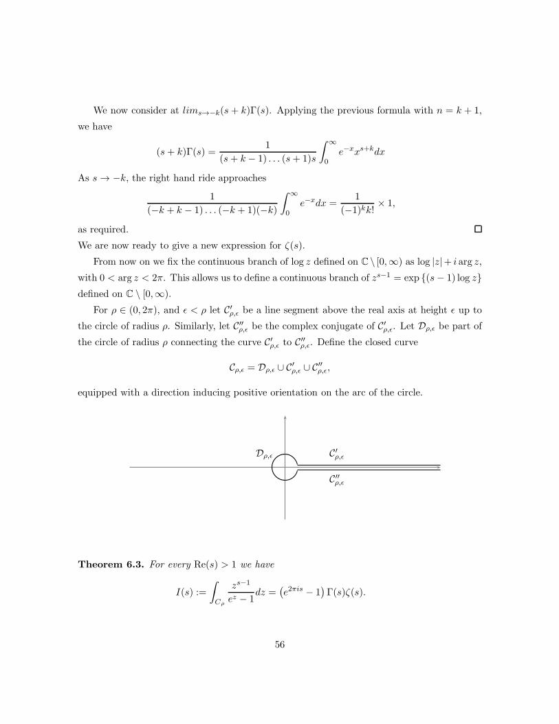
We now consider at lims→−k(s + k)Γ(s). Applying the previous formula with n = k + 1,
we have
(s+ k)Γ(s) =1
(s+ k − 1) . . . (s+ 1)s
ˆ ∞
0e−xxs+kdx
As s→ −k, the right hand ride approaches
1
(−k + k − 1) . . . (−k + 1)(−k)
ˆ ∞
0e−xdx =
1
(−1)kk!× 1,
as required.
We are now ready to give a new expression for ζ(s).
From now on we fix the continuous branch of log z defined on C \ [0,∞) as log |z|+ i arg z,with 0 < arg z < 2π. This allows us to define a continuous branch of zs−1 = exp {(s− 1) log z}defined on C \ [0,∞).
For ρ ∈ (0, 2π), and ǫ < ρ let C′ρ,ǫ be a line segment above the real axis at height ǫ up to
the circle of radius ρ. Similarly, let C′′ρ,ǫ be the complex conjugate of C′
ρ,ǫ. Let Dρ,ǫ be part of
the circle of radius ρ connecting the curve C′ρ,ǫ to C′′
ρ,ǫ. Define the closed curve
Cρ,ǫ = Dρ,ǫ ∪ C′ρ,ǫ ∪ C′′
ρ,ǫ,
equipped with a direction inducing positive orientation on the arc of the circle.
Dρ,ǫ C′ρ,ǫ
C′′ρ,ǫ
Theorem 6.3. For every Re(s) > 1 we have
I(s) :=
ˆ
Cρ
zs−1
ez − 1dz =
(
e2πis − 1)
Γ(s)ζ(s).
56
Proof
The integrand is meromorphic on C \ [0,∞), with poles at 2πin, for every nonzero integer
n. If we vary ρ within the range 0 < ρ < 2π (with ǫ < ρ) the integral does not change, by
Cauchy’s theorem. On Dρ,ǫ we have |z| = ρ and
|ez − 1| =∣
∣
∣
∣
z +z2
2+z3
6+ . . .
∣
∣
∣
∣
= |z|∣
∣
∣1 +z
2+ . . .
∣
∣
∣ ≥ |z|2
=ρ
2,
if ρ is small enough. Moreover
∣
∣zs−1∣
∣ = |exp{(s− 1) log z}| = exp {Re((s− 1) log z)}
= exp {(σ − 1) log |z| − t arg z} ≤ exp {(σ − 1) log ρ+ 2π|t|}
= ρσ−1e2π|t|.
Hence∣
∣
∣
∣
∣
ˆ
Dρ,ǫ
zs−1
ez − 1dz
∣
∣
∣
∣
∣
≤ 2πρρσ−1e2π|t|
12ρ
= 4πρσ−1e2π|t| → 0
as ρ→ 0, since σ > 1. Thus, as ρ and ǫ tend to zero,
I(s) =
ˆ
C′
ρ,ǫ
zs−1
ez − 1dz +
ˆ
C′′
ρ,ǫ
zs−1
ez − 1dz
= −ˆ ∞
0
xs−1
ex − 1dx+ e2πi(s−1)
ˆ ∞
0
xs−1
ex − 1dx,
since on C′′ρ,ǫ, as ǫ→ 0, we have
zs−1 = e(s−1)(log |z|+iarg z)
= e(s−1)(log x+2πi)
= xs−1e2πi(s−1) = e2πis.
Hence
I(s) =(
e2πis − 1)
ˆ ∞
0
xs−1
ex − 1dx.
Finally,1
Y − 1= Y −1 + Y −2 + . . .
57
for Y > 1 so that
ˆ ∞
0
xs−1
ex − 1dx =
ˆ ∞
0xs−1
{
e−x + e−2x + . . .}
dx
=∞∑
n=1
ˆ ∞
0xs−1e−nxdx
providing that we can interchange summation and integration. This is permissible if
∞∑
n=1
ˆ ∞
0
∣
∣xs−1e−nx∣
∣ dx
converges. However
ˆ ∞
0
∣
∣xs−1e−nx∣
∣ dx =
ˆ ∞
0xσ−1e−nxdx = n−σ
ˆ ∞
0yσ−1e−ydy = n−σΓ(σ),
and∑
n−σ <∞, since σ > 1. We are therefore able to deduce that
ˆ ∞
0
xs−1
ex − 1dx =
ˆ ∞
0xs−1
{
e−x + e−2x + . . .}
dx
=∞∑
n=1
ˆ ∞
0xs−1e−nxdx
=
∞∑
n=1
n−sˆ ∞
0ys−1e−ydy
= ζ(s)Γ(s).
The theorem now follows.
Previously we showed how to extend our original definition of ζ(s) from the region σ > 1
to the larger region σ > 0. We can now go much further, by providing a meaningful definition
over the whole complex plane.
Corollary 6.4. The function(
e2πis − 1)
ζ(s)Γ(s) has an analytic continuation as an entire
function on C. Thus ζ(s) has a continuation as a meromorphic function on C, the only
possible poles being the points where(
e2πis − 1)
Γ(s) = 0.
Proof
First we show that the integral I(s) represents a well-defined function of s (with finite complex
58
values). Recall that the value of the integral is independent of the choice of ρ ∈ (0, 2π), so
we may as well work with some value of ρ ≥ 1. Indeed, we show that the integral converges
uniformly in any disc |s| ≤ R.
Fix s ∈ C with |s| ≤ R. Since for z ∈ Cρ,ǫ, |z| ≥ 1, we have
∣
∣
∣
∣
zs−1
ez − 1
∣
∣
∣
∣
≤ |z|σ−1e2π|t|
|ez − 1| ≤ |z|R−1e2πR
|ez − 1| .
Moreover the function |z|R−1e2πR|ez − 1|−1 has a finite integral along the paths
ˆ
Dρ,ǫ
|z|R−1e2πR
|ez − 1| |dz|
andˆ
C′
ρ,ǫ or C′′
ρ,ǫ
|z|R−1e2πR
|ez − 1| |dz| ≤ O(
ˆ ∞
0
xR−1e2πR
ex − 1dx)
are finite.
In general if G(z, s) is an entire function of s that has uniformly bounded integrals´
γ G(z, s) dz on some curve γ ⊂ C, the function H(s) =´
γ G(z, s) dz is an entire function
of s. Here, since zs−1/(ez − 1) is an entire function of s, we conclude that I(s) is entire.
One can check that the function zez−1 + z
2 is an even function of z. Define the Bernoulli
Numbers Bm by
z
ez − 1+
1
2z = 1 +B1
z2
2!−B2
z4
4!+B3
z6
6!− . . . .
We can also check that Bm are all rational numbers and that
B1 =1
6, B2 =
1
30, B3 =
1
42, . . . .
In fact the numbers Bm are all positive. The Bernoulli numbers appear in subjects of combi-
natorics, probability, and number theory.
Corollary 6.5. We have,
a) ζ(0) = −12 ;
b) ζ(−2m) = 0 for all m ∈ N;
59
c) ζ(1− 2m) = (−1)mBm
2m , for all m ∈ N.
Remark. The above result shows in particular that ζ(−k) ∈ Q for all k ∈ Z≥0.
Proof
Take k ∈ Z≥0. By Corollary 6.2 Γ(s) has a singularity of order 1 at −k, with residue (−1)k/k!.
Also e2πis − 1 has a simple zero at −k, with e2πis−1s+k → 2πi as s → −k. Hence as s → −k we
have
Γ(s)(
e2πis − 1)
→ 2πi(−1)k
k!.
Now I(s) = Γ(s)(e2πis − 1)ζ(s) and I(s) is continuous at s = −k, so that
ζ(−k) = k!
2πi(−1)kI(−k).
However
I(−k) =ˆ
Cρ
z−k−1
ez − 1dz
with Cρ as before. Since k is integer, the function z−k−1 extends from C− [0,∞) to C− {0}as a continuous function and
ˆ +ρ
+∞arg z=0
z−k−1
ez − 1dz = −
ˆ +∞
+ρarg z=2π
z−k−1
ez − 1dz.
It follows that
I(−k) =
˛
|z|=ρ
z−k−1
ez − 1dz
=
˛
|z|=ρz−k−2
(
z
ez − 1
)
dz
=
˛
|z|=ρz−k−2
(
1− 1
2z +
B1
2!z2 − B2
4!z4 + . . .
)
dz
= 2πic,
where c is the coefficient of z−1 in
z−k−2
(
1− 1
2z +
B1
2!z2 − B2
4!z4 + . . .
)
.
60
It follows that
c =
−12 , k = 0,
0, k = 2m > 0,
(−1)m−1
(2m!) Bm, k = 2m− 1 > 0.
Hence ζ(−k) = (−1)kk!2πi I(−k), which is −1
2 , or 0 or (−1)m
2m Bm in the three cases.
We next give an alternative evaluation of I(s), which leads to a new connection with the
zeta-function.
Proposition 6.6. If σ < 0 then I(s) = eiπs/2(eiπs − 1)(2π)sζ(1− s).
Proof
Fix ǫ < 1. We define a new contour Cn, for n ∈ N, starting at +∞+ǫi, running to (2n+1)π+ǫi
(above the real axis), along the line segments
(2n + 1)π + ǫi→ (2n+ 1)π(1 + i) → (2n+ 1)π(−1 + i)
→ (2n+ 1)π(−1 − i) → (2n + 1)π(1 − i) → (2n + 1)π − ǫi,
and back to +∞− ǫi just below the real axis. It will be convenient to write Sn for the part
of the contour running around the square from (2n + 1)π + ǫi to (2n + 1)π − ǫi.
We now replace the contour Cρ by Cn. The integrandzs−1
ez−1 has poles at 2πik for k ∈ Z−{0}.Hence, by Cauchy’s residue theorem, we have
I(s) =
ˆ
Cρ
zs−1
ez − 1dz
=
ˆ
Cn
zs−1
ez − 1dz −
∑
1≤|k|≤n2πiRes
(
zs−1
ez − 1; z = 2πik
)
.
However, if k > 0,
Res
(
zs−1
ez − 1; z = 2πik
)
= limz→2πik
zs−1(z − 2πik)
ez − 1=e(s−1)(log 2πk+iπ
2)
1,
and similarly, for k > 0,
Res
(
zs−1
ez − 1; z = −2πik
)
= e(s−1)(log 2πk+3iπ2).
61
It follows that
I(s) =
ˆ
Cn
zs−1
ez − 1− 2πi
n∑
k=1
(2πk)s−1(
e(s−1)iπ/2 + e(s−1)3iπ/2)
=
ˆ
Cn
zs−1
ez − 1− 2πi
(
eiπs/2(−i) + e3iπs/2i)
n∑
1
(2πk)s−1
=
ˆ
Cn
zs−1
ez − 1+ (2π)s
(
eiπs − 1)
eiπs/2n∑
1
ks−1.
We now allow n to tend to infinity. On the contour Cn the function 1ez−1 is bounded from
above independently of n or z, since ez − 1 is bounded away from zero. Moreover
|zs−1| = eRe((s−1) log z) = e(σ−1) log |z|−targ z ≤ e(σ−1) log |z|+2π|t|,
whence |zs−1| ≤ e2π|t||z|σ−1. So on Sn, which was the square part of the contour, we have
|zs−1| = O(nσ−1), whenceˆ
Sn
zs−1
ez − 1dz = O(nnσ−1) = O(nσ).
This tends to zero as n goes to infinity, since σ < 0. Moreover, whether we take arg(z) = 0
or 2π, we will have
ˆ ∞
(2n+1)π
zs−1
ez − 1dz = O
(
ˆ ∞
(2n+1)π|z|σ−1dz
)
= O
(
ˆ ∞
(2n+1)πxσ−1dx
)
= O
(
[
xσ
σ
]∞
(2n+1)π
)
= O (((2n + 1)π)σ) ,
and this also tends to 0 when σ < 0.
We therefore conclude thatˆ
Cn
zs−1
ez − 1dz → 0 as n→ ∞
so that
I(s) = (2π)seiπs/2(
eiπs − 1)
∞∑
1
ks−1.
62
This completes the proof, since∑∞
1 ks−1 = ζ(1− s) for Re(s) < 0.
Corollary 6.7. (The Functional Equation for ζ(s)). We have
ζ(1− s) = 21−sπ−s cos(πs
2
)
Γ(s)ζ(s)
for all s ∈ C − {0}. Moreover ζ(s) is meromorphic on C, with the only singularity being a
simple pole at s = 1.
Proof
If σ < 0 then
ζ(1− s) = (2π)−se−iπs/21
eiπs − 1I(s)
when 12s /∈ Z. According to Theorem 6.3 and Corollary 6.4 we have I(s) =
(
e2πis − 1)
Γ(s)ζ(s)
on the complex plane, so that
ζ(1− s) = (2π)−se−iπs/21
eiπs − 1
(
e2πis − 1)
Γ(s)ζ(s)
= (2π)−s(eπis/2 + e−πis/2)Γ(s)ζ(s)
= 21−sπ−s cos(πs
2)Γ(s)ζ(s),
using the definition cos(z) = (eiz + e−iz)/2 on the complex plane.
Now define f(s) = ζ(1− s)− 21−sπ−s cos πs2 Γ(s)ζ(s). This is meromorphic and it vanishes
on D(−1, 1), for example. Here D(−1, 1) denotes the open disk of radius +1 about −1 within
C. Hence, by the Identity Theorem we have f(s) = 0 for all s ∈ C.
Finally, from Theorem 4.2 we know that ζ(s) is meromorphic for σ > 0, with the only
singularity being a simple pole at s = 1. Thus when σ > 0 the function ζ(s) cos πs2 is holomor-
phic, since cos πs2 has a zero at s = 1. It follows that 21−s cos πs2 Γ(s)ζ(s) is holomorphic for
σ > 0. We deduce that ζ(1−s) is holomorphic for s > 0. This means that ζ(s) is holomorphic
in the region σ < 1. Since ζ(s) is also regular for σ > 0, apart from the pole at s = 1, we
deduce that ζ(s) is regular everywhere, apart from the point s = 1.
Corollary 6.8. If ζ(s) = 0 then either s = −2,−4,−6, . . ., or s lies in the “critical strip”
0 < Re(s) < 1.
63
Proof
If σ ≥ 1, then ζ(s) 6= 0, by Theorem 4.1 (for σ > 1) and Theorem 4.5 (for σ = 1).
If ζ(s) = 0 with σ ≤ 0, then Corollary 6.7 tells us that either ζ(1 − s) vanishes, or
21−sπ−s cos πs2 Γ(s) has a pole. However ζ(1− s) 6= 0 since Re(1 − s) ≥ 1. Moreover the only
possible poles of 21−sπ−s cos πs2 Γ(s) are those of Γ(s), which lie at s = 0,−1,−2, . . .. When
s = −n with n odd, the pole of Γ(s) is cancelled by a zero of cos πs2 , so that the only possibility
left is that s = −n with n > 0 even. According to Corollary 6.5 these points are indeed zeros
of ζ(s).
Going back to the starting argument on the zeros of ζ(s) at the beginning of the section,
of course all this effort would be pointless if ζ(s) had no zeros in the critical strip, but in
fact there are infinitely many such zeros, and they are a fundamental obstruction to our
understanding of the primes.
We can say a little more about the zeros of ζ(s). In particular,
Corollary 6.7 tells us that if s is in the critical strip then ζ(s) = 0 if and only if ζ(1−s) = 0.
However something further is true.
Theorem 6.9. We have ζ(s) = ζ(s) for all s ∈ C− {1}.
Lemma. If f(s) is meromorphic on C, then so is f∗(s) := f(s).
Proof
Easy exercise, using the fact that
limh→0
f∗(s+ h)− f∗(s)h
= f ′(s).
We can now prove Theorem 6.9.
Proof
Set F (s) = ζ(s)− ζ(s), which will be meromorphic on C by the above lemma. When s is real
we have s = σ, and F (σ) = ζ(σ)− ζ(σ) = 0. Thus F (s) vanishes on the real axis, and hence
by the Identity Theorem F (s) = 0 for all s.
64
Corollary 6.10. If ζ(ρ) = 0 with ρ in the critical strip, then each of ρ, 1 − ρ, ρ and 1− ρ is
a zero of ζ(s).
Proof
This follows from Theorem 6.9 and Corollary 6.7.
We conclude with various remarks:- Corollary 6.10 suggests that the zeros occur in groups
of 4, unless ρ is real or Re(ρ) = 1/2. In fact one can show thatζ(s) 6= 0 for real s ∈ (0, 1).
Indeed it appears that all zeros in the critical strip have Re(s) = 1/2 (so that the zeros are
only in pairs, s and 1− s (= s)).
It is known that ζ(s) has infinitely many zeros in the critical strip. Up to height Im(s) = T
there are around T2π log T such zeros.
The first zero is about 12 ± (14.13 . . .)i and the next ones are roughly
1
2± (21.02 . . .)i,
1
2± (25.01 . . .)i,
1
2± (30.42 . . .)i,
1
2± (32.93 . . .)i,
1
2± (37.58 . . .)i.
They are irregularly spaced.
Calculations show that Re(s) = 12 for all zeros in the critical strip with 0 < Im(s) < 1012,
in which range there are over 1013 zeros.
All this evidence points to the following statement, whose proof would have far-reaching
consequences for our knowledge of prime numbers.
The Riemann Hypothesis If ζ(s) = 0 and 0 < Re(s) < 1 then Re(s) = 1/2.
65
7 References
• T. M. Apostol, Introduction to Analytic Number Theory
• H. Davenport, Multiplicative Number Theory
• G. H. Hardy and E. M. Wright, An Introduction to the Theory of Numbers
• I. Niven, H. S. Zuckerman, and H. L. Montgomery, An Introduction to the Theory of
Numbers
• L. V. Ahlfors, complex analysis
• G. B. Foland, Real analysis; modern techniques and their applications
66