Rank-Based Ant Colony Algorithm For A Thermal Generator ... · PDF fileRank-Based Ant Colony...

Rank-Based Ant Colony Algorithm For A Thermal Generator Maintenance Scheduling Problem

ARISTIDIS VLACHOS

Department of Informatics University of Piraeus

80 Karaoli and Dimitriou Street,18534,Piraeus GREECE

Α[email protected]

Abstract:The maintenance scheduling of thermal generators is a large-scale combinatorial optimization problem with constraints. In this paper we introduce the Rank-Based Ant System algorithm based version of the Ant System. This algorithm reinforces local search in neighborhood of the best solution found in each iteration while implementing methods to slow convergence and facilitate exploration.Rank-Based Ant System (RBAS) algorithm has been proved to be very effective in finding optimum solution to hard combinational optimization problems . To show its efficiency and effectiveness, the proposed Rank-Based Ant System algorithm is applied to a real-scale system, and further experimenting leads to results that are commented. Key-Words: thermal generator maintenance scheduling problem; ant colony optimization; ant system,rank-based ant system algorithm

1.Introduction The Thermal Generator Maintenance Scheduling Problem is a complex multivariable problem that is necessary for the reliability and right operation of a generator system, given that the whole production cost is dependent on the maintenance and operation cost. Thus, the maintenance procedure has to be scheduled and complied with the best possible way, minimizing these two costs and at the same time, covering the energy demands, so as every constraint of the problem is satisfied. The problem has been studied in the past with a variety of modeling methods. The initial formulation was made by Gruhl [1], [2]. He presented an umbrella of scheduling problems, one of which was the generator maintenance scheduling problem, with a linear approach. Two years later, Dopazo and Merill [3] developed a model which was claimed to

have the ability of finding the best solution, but this approach was lacking in real-scale problems application, something that Zurn and Quintana [4] later achieved to do using computational methods. In 1983, Yamayee and Sidenblad [5] improved the cost function that was used till then, with great improvements in execution time. In 1991, Satoh and Nara [6] applied for the first time a stochastic method, called Simulated Annealing with very good results in large-scale systems as well, that were impossible to be solved with linear methods in the past. They also investigated the problem with genetic algorithms [7] and tabu-list methods [8] with similar results, but with the ability to solve real-scale problems, too. In 1993, Charest and Ferland [9] tried to modify the linear method with successful results in execution time, while Dahal and McDonald [10] applied a genetic algorithm in Boolean representation [11] which had

WSEAS TRANSACTIONS on CIRCUITS and SYSTEMS Aristidis Vlachos

E-ISSN: 2224-266X 273 Issue 9, Volume 12, September 2013

mailto:Α[email protected]

also some good results. In 1997, Burke and Smith [12] tried to create a hybrid model of the simulated annealing and the tabu-list method without success, following another attempt to make another hybrid model with memetic and tabu-list methods three years later, which resulted in better results, but with a small increase in execution time. In 2010 Y.Yare.,G.K.Venayagamoorthy [13] using multiple swarms-MDPSO framework with good results for Optimal maintenance scheduling of generators problem. In 2011, Saraiva, Pereiva, Mendes, and Sousa [14] solved the generator maintenance scheduling problem using a simulated annealing algorithm. In this paper, we introduce Rank-Based Ant System algorithm [15], an imported version of basic Ant System [16] of the family algorithms: Ant Colony Optimization (ACO) [17], which was inspired by the observation of ant colonies.

2.Ant Colony Optimization 2.1 Generally Analogy The Ant Colony Optimization (ACO) [18] is a metaheuristic to solve combinatorial optimization problems, is motivated by the behavior of real ant colonies. When ants attempt to find short paths between their nest and food sources, they communicate indirectly by using pheromone (pheromone trail) to mark the decisions they made when building their respective paths. Within ACO algorithms, the optimization problem is represented as a complete weighted graph G = (N,A) with N being the set of nodes and A the set of edges fully connecting the nodes N. In the Travelling Salesman Problem (TSP) application, edges have a cost associated (e.g. their length) and the problem is to find a minimal-length closed tour that visits all the nodes once and only once. In order to solve the problem, random walks of a fixed number of ants through the graph take

place. The transition probabilities of each ant are governed by two parameters associated to the edges of the graph: the pheromone values (or pheromone trail) τij, representing the learned desirability of choosing node j when in node i. inverse of the distance between two nodes i and j:

1ij

ij

n =d

where ijd is the distance between

these two nodes. The more distinctive feature of ACO is the management of pheromone trails that are used, in conjunction with the objective function, to construct new solutions. Informally, the pheromone trails are used for exploration and exploitation. Exploration representing the probabilistic choice of the components used to construct a solution. A higher probability is given to elements with a strong pheromone trail. Exploitation is based on the choice of the component that maximizes ablend of pheromone-trail values and partial objective function evaluations. The mathematical formulations of the ACO algorithms presented in this paper named Ant System (AS) and Max-Min Ant System (MMAS), are given in the following sections. 2.2 Ant System Ant System (AS) [19] is the original and most simplistic ACO algorithm. The decision policy used within AS is as follows: The probability with which ant k, currently at node i, chooses to go to node j is given [16] by:

(1) [ ] [ ]

( )1α β

ij ijkij α β

ιl ilkl Ji

τ (t) np (t)=

τ (t) n∈

⋅ ⋅∑

If j є k

iJ and 0 if kij J∉



:kiJ is the feasible neighborhood of ant k,

that is, the set of nodes which ant k has not yet visited.

ijτ (t) : is the concentration of pheromone associated with edge (i,j) in iteration t.

:ijn is the inverse of the length of the edge known as visibility α and β: are parameters that control the relative importance of pheromone intensity versus visibility Upon conclusion of an iteration (i.e. each ant has generated a solution) the pheromone on each edge is updated, according to the following formula: (2) ( )2ij ij ijτ (t)= ρτ (t)+ Δτ (t) Where ρ is the coefficient representing pheromone persistence (0 ≤ ρ < 1), and

ijΔτ , is a function of the solutions found at iteration t, given by:

(3) ( )1

3n

kij ij

k=Δτ = Δτ (t)∑

n: number of ants

:kijΔτ is the quantity per unit of length of

pheromone addition laid on edge (i,j) by the kth ant at the end of iteration t, is given by: Where kT (t) is the tour done by ant k at iteration t, kL (t) , is its length and Q is a constant parameter, used for defining to be of high quality solutions with low cost. (4)

( ), if ( , ) ( )( ) (4) 0, if ( , ) ( )

k kkij

k

QL t i j T tt

i j T tτ

∈∆ = ∉

2.3 Rank-Based Ant System Algorithm (Bullnheimer,Hartl and Strauss) [15],proposed the RBAS algorithm which is a modification of the AS algorithm. The

RBAS algorithm uses a rank idea to update the pheromone trail. The RBAS search mechanism can be divided into :

(1) Initialization. (2) Transition rule. (3) Pheromone update

rule. (1) Initialization. The pheromone initialization strategy is to initialize the pheromone matrix of RBAS algorithm. As elements using a constant value [19,20,21]: (5) ( )0 5ijτ τ , i, j← ∀

(2) Transition rule. Let denote for each arc (i,j) in the TSP-instance graph a heuristic value and pheromone value. Ant k at node I chooses next node j according the following transition rule .

(6) β

iu iu 0u

0

arg max [η ] }, q q

,

kiJ

ifj

J if q q

τ∈

≤= >

And J in kiJ is a node that is randomly

selected according to the probability :

(7) ( ) ( ) [ ]( ) [ ]

( )7α β

iJ iJα β

il il

τ t nkP t =

ij τ t n

⋅ ⋅ ∑

Where q is a random variable uniformly distributed over [0,1], 0q is a parameter



( 00 1q≤ ≤ ) .The value of parameters α and β ( 0α > , 0β > ),determines the relative importance of pheromone and heuristic information (visibility). When 0q is equal to 1, the ants will exploit the known information about the nodes and the pheromone whereas,when 0q is equal to 0,the ants will splore more in the neighborhood of node i. (3) Pheromone update rule. The difference between the Ant System (AS) and Rank-Based Ant System (RBAS) algorithm is : • In the RBAS algorithm each ant

deposits a quantity of pheromone that decreases with rank.

• The amount of pheromone an ant deposits is weighted according to the rank of the ant.

• In its iteration only the Λ = σ – 1 best-ranked ants and the ant that produced are allowed to deposit the pheromone.

In RBAS algorithm the pheromone level is updated as follows: (8) ( ) ( ) ( ) ( )11 8ij ij i

k

τ t+ τ t + σ λL

← − ⋅

Where : kL : is the cost of the solution.

σ : is the weight of the pheromone witch corresponding in the best-so-far tour

iσ λ− : is the weight for iλ th− best ant. Λ = σ - 1: is the number of the best ants that generated the best-so-far tour.. After each iteration of the RBAS algorithm,when all ants have built a route-solution an a local update procedure can be performed reducing the quantity of pheromone in corresponding route using a parameter ξ : 0 1< ξ ≤ according to the expression [9] :

(9) ( ) ( )9ij ijτ t ξ τ← ⋅ Finally, for all routes-solutions the pheromone trail reduces as follows: (10) ( ) ( ) ( ) ( )1 10ij ijτ t τ tρ← − ⋅ The ρ∈(0,1) is called evaporation coefficient. 3.Formulation of the problem The objective of the Thermal Generator Maintenance Scheduling Problem is the maintenance of the energy production units of a system in a given horizon, with the lowest possible cost. The list of symbols that describe the problem is as follows[22,23]: i : Number of generator Ι : Number of generators j : Number of week xi : Maintenance start period; xi ∈ {1,2, …,J} J : Horizon in weeks Xi : Set of proposed maintenance start periods in weeks Mi : Maintenance length in weeks Yij : State variable:

1 , int

0 ,ij

if unit i is in ma enanceat period jotherwise

−Υ =

pij : power output of unit-i at period-j fi : fuel cost coefficient (linear cost function) ci(xi) : maintenance cost of unit-i when the maintenance is committed at period ix Pi : capacity of unit i Dj : anticipated power demand at period-j Rj : required power reserve at period-j The generator maintenance scheduling problem is formulated as shown below: Objective function



The objective is to minimize the objective function which is the sum of the following two terms:

(12) 1 1 1

niI J I

M i ij i ii= j= i=

f p + c (x )

⋅

∑∑ ∑

Where the first term is the production cost and the second is the maintenance cost. Constraints

1) The nominal starting period of maintenance is pre-specified for each generating unit: (13) { }1,2 ...i ix X , ,J∈ ⊆

2) Once the maintenance of unit-i starts, the unit must be in the maintenance state for just iM periods:

(14) 0, 1, 2,..., 11, ,..., 10, ,...,

i i i

i i

j xij j x x M

j x M J

= −Υ = = + − = +

3) If unit- 1i and unit- 2i cannot be

maintained in a given week because of the crew constraint, the following constraint is imposed:

(15) 1 1,2 ...(i1)j (i2)jY +Y , j = , ,J≤

4) If the maintenance of unit- 1i must be finished prior to the starting of that of unit- 2i , the following constraint is added:

(16) i1 i1 i2x + M x≤

5) The generator output must be less than its upper limit; and the output of the generator in maintenance must be equal to zero. Such an operation constraint is expressed by:

(17) 0 1 1,... 1,...ij i ijp P ( y ) , i = ,I, j = ,J≤ ≤ ⋅ −

6) The demand constraint must be met:

(18) 1

1,2 ...I

ij ji=

p = D , j = , ,J∑

7) In order to ensure that the total

available power is greater than the demand jD even when a unit random outage occurs, the reserve constraints are imposed. That is, the total available power from units which are not committed must be greater than the demand plus reserve:

(19) 1

1 1,2 ...I

i ij j ji=

P ( y ) D + R , j = , ,J⋅ − ≥∑ Penalty Function In the generator maintenance scheduling problem, the constraints are classified into two groups; “easy” constraints and “difficult” constraints. The easy constraints are equations (13), (14), (16), (17), the difficult constraints are equations (15), (18), (19). Since the set iX is given, the value of ix can be selected as a member of

iX so that equations (13), (16) are satisfied. Then the value of ijy is directly defined by equation (14), and equation (17) becomes a simple bound on ijp . On the other hand, it is very difficult to find a feasible solution which satisfies equations(15), (18) and (19). So, the artificial variables iz , iu , and iv are introduced corresponding to equations (15), (18) and (19), with associated positive penalty parameters α, β, and γ. Then the problem is re-formulated as follows:



(20)

⋅+⋅+⋅+

+⋅

∑ ∑∑

∑∑∑

= ==

== =

J

j

J

jii

J

ji

i

I

ii

I

ii j

J

ji

vuz

xcpf

M i n1 11

11 1)(

γβα

(21) { }1,2 ...i ix X , ,J∈ ⊆

(22) 0, 1, 2,..., 11, ,..., 10, ,...,

i i i

i i

j xij j x x M

j x M J

= −Υ = = + − = +

(23) 1 1,2 ...(i1)j (i2)j jY +Y z , j = , ,J− ≤ (24) i1 i1 i2x + M x≤ (25) 0 1 1,... 1,...ij i ijp P ( y ) , i = ,I, j = ,J≤ ≤ ⋅ −

(26) 1

1,2 ...I

ij j ji=

p +u = D , j = , ,J∑

(27)

11 1,2 ...

I

i ij j j ji=

P ( y )+v D + R , j = , ,J⋅ − ≥∑

(28) { }0,1nz ∈ (29) 0 1,2 ...j j ju , v , j = , ,J≥ By using the above formulation, once the value of ix is determined, the value of ijy is directly defined, and the value of ijp is calculated through the equal incremental method λ for the economic dispatch problem [24]. Therefore, the value of the objective function can be efficiently evaluated if the value of ix is specified. 4. Implementation of RBAS algorithm for the generator maintenance scheduling

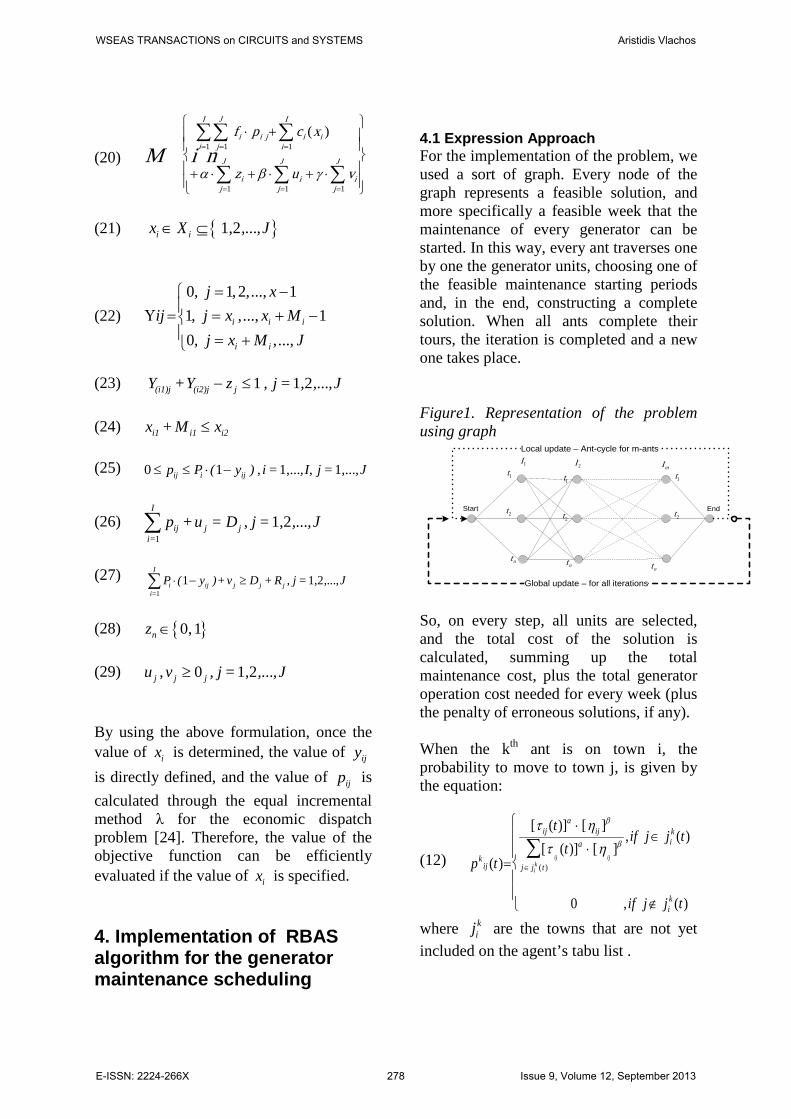
4.1 Expression Approach For the implementation of the problem, we used a sort of graph. Every node of the graph represents a feasible solution, and more specifically a feasible week that the maintenance of every generator can be started. In this way, every ant traverses one by one the generator units, choosing one of the feasible maintenance starting periods and, in the end, constructing a complete solution. When all ants complete their tours, the iteration is completed and a new one takes place. Figure1. Representation of the problem using graph

1I2I

mI1t

Local update – Ant-cycle for m-ants

2t

nt

Start End

1t

2t

1t

2t

ntnt

Global update – for all iterations

So, on every step, all units are selected, and the total cost of the solution is calculated, summing up the total maintenance cost, plus the total generator operation cost needed for every week (plus the penalty of erroneous solutions, if any).

When the kth ant is on town i, the probability to move to town j, is given by the equation:

(12)

pkij (t)=

[τ ij (t)]a ⋅ [ηij ]

β

[τij(t)]a ⋅ [η

ij]β

j ∈ jik (t )

∑,if j ∈ ji

k (t)

0 ,if j ∉ jik (t)

where kij are the towns that are not yet

included on the agent’s tabu list .



As visibility ijη between towns, we will

use the equation 11ij

ij

η (t)=+ PCV (t)

where ij

PCV (t) is a method counting the

total number of the Problem Constraint Violations. We will bias each constraint violation using weights which correspond to the relative importance of each constraint. Thus, each ant will be guided as to not choose the towns that violate the problem’s constraints. 4.2 The Algorithm 1. Define problem parameters for each agent and generator. 2. Calculation of the first solution for each unit. 3.Evaluation of the solution constructed by each ant and classification of the ants according to the solution they found. 4. Renewal of the amount of pheromone from the ants that found the best solutions. 5. Pheromone reduction in the best routes-solutions according to factor ξ. 6. Global pheromone reduction according to factor p. 7. Select a new ant. 8. Repeat the algorithm from step 3 until a specific number of iterations is completed, or a criterion of convergence is satisfied. 5.Case study on a real – scale system of generators The algorithm just described, was implemented on a real scale system of generator units [25] with 22 power generator units that have to be maintained within a 52-week horizon.

The following table shows the parameters that describe every generator unit’s operation and maintenance:



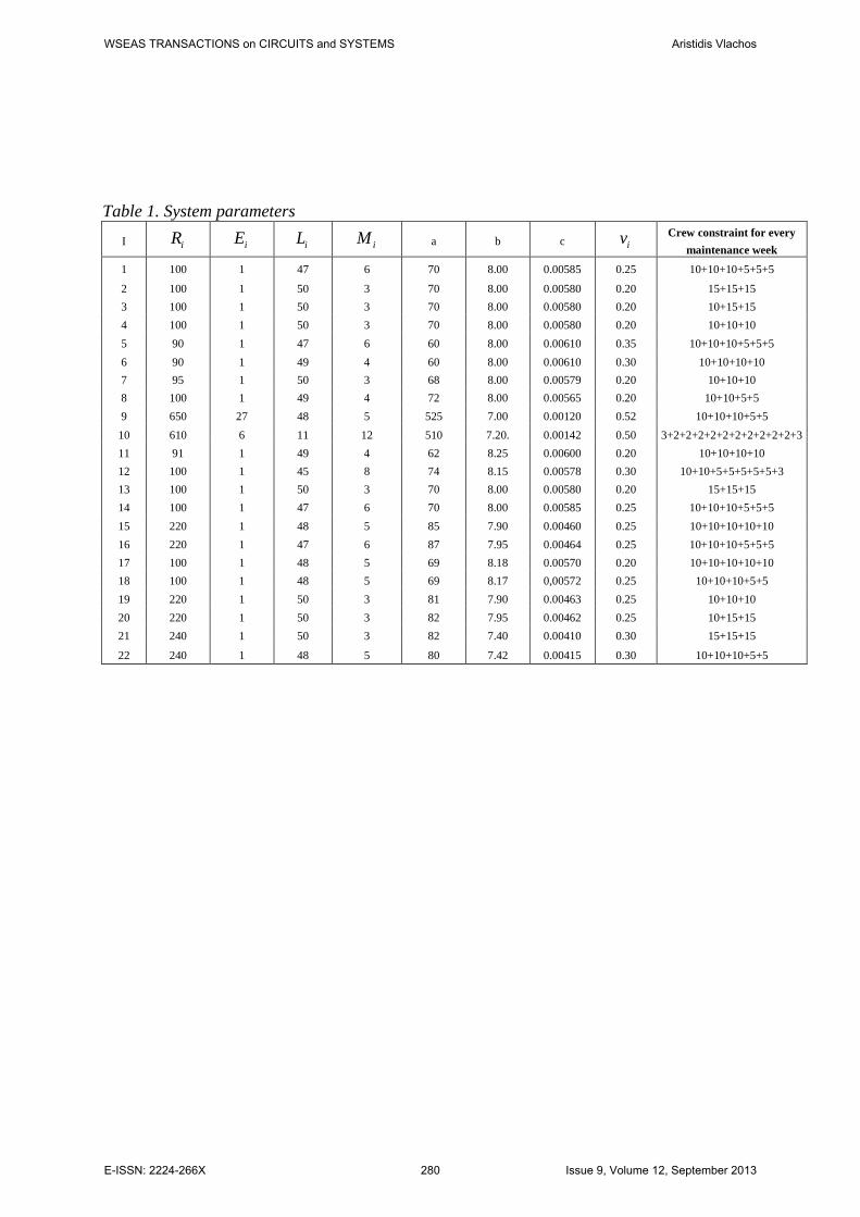
Table 1. System parameters Ι iR iE iL iM a b c iv Crew constraint for every

maintenance week 1 100 1 47 6 70 8.00 0.00585 0.25 10+10+10+5+5+5

2 100 1 50 3 70 8.00 0.00580 0.20 15+15+15 3 100 1 50 3 70 8.00 0.00580 0.20 10+15+15 4 100 1 50 3 70 8.00 0.00580 0.20 10+10+10 5 90 1 47 6 60 8.00 0.00610 0.35 10+10+10+5+5+5 6 90 1 49 4 60 8.00 0.00610 0.30 10+10+10+10 7 95 1 50 3 68 8.00 0.00579 0.20 10+10+10 8 100 1 49 4 72 8.00 0.00565 0.20 10+10+5+5 9 650 27 48 5 525 7.00 0.00120 0.52 10+10+10+5+5

10 610 6 11 12 510 7.20. 0.00142 0.50 3+2+2+2+2+2+2+2+2+2+2+3 11 91 1 49 4 62 8.25 0.00600 0.20 10+10+10+10 12 100 1 45 8 74 8.15 0.00578 0.30 10+10+5+5+5+5+5+3 13 100 1 50 3 70 8.00 0.00580 0.20 15+15+15 14 100 1 47 6 70 8.00 0.00585 0.25 10+10+10+5+5+5 15 220 1 48 5 85 7.90 0.00460 0.25 10+10+10+10+10 16 220 1 47 6 87 7.95 0.00464 0.25 10+10+10+5+5+5 17 100 1 48 5 69 8.18 0.00570 0.20 10+10+10+10+10 18 100 1 48 5 69 8.17 0,00572 0.25 10+10+10+5+5 19 220 1 50 3 81 7.90 0.00463 0.25 10+10+10 20 220 1 50 3 82 7.95 0.00462 0.25 10+15+15 21 240 1 50 3 82 7.40 0.00410 0.30 15+15+15

22 240 1 48 5 80 7.42 0.00415 0.30 10+10+10+5+5



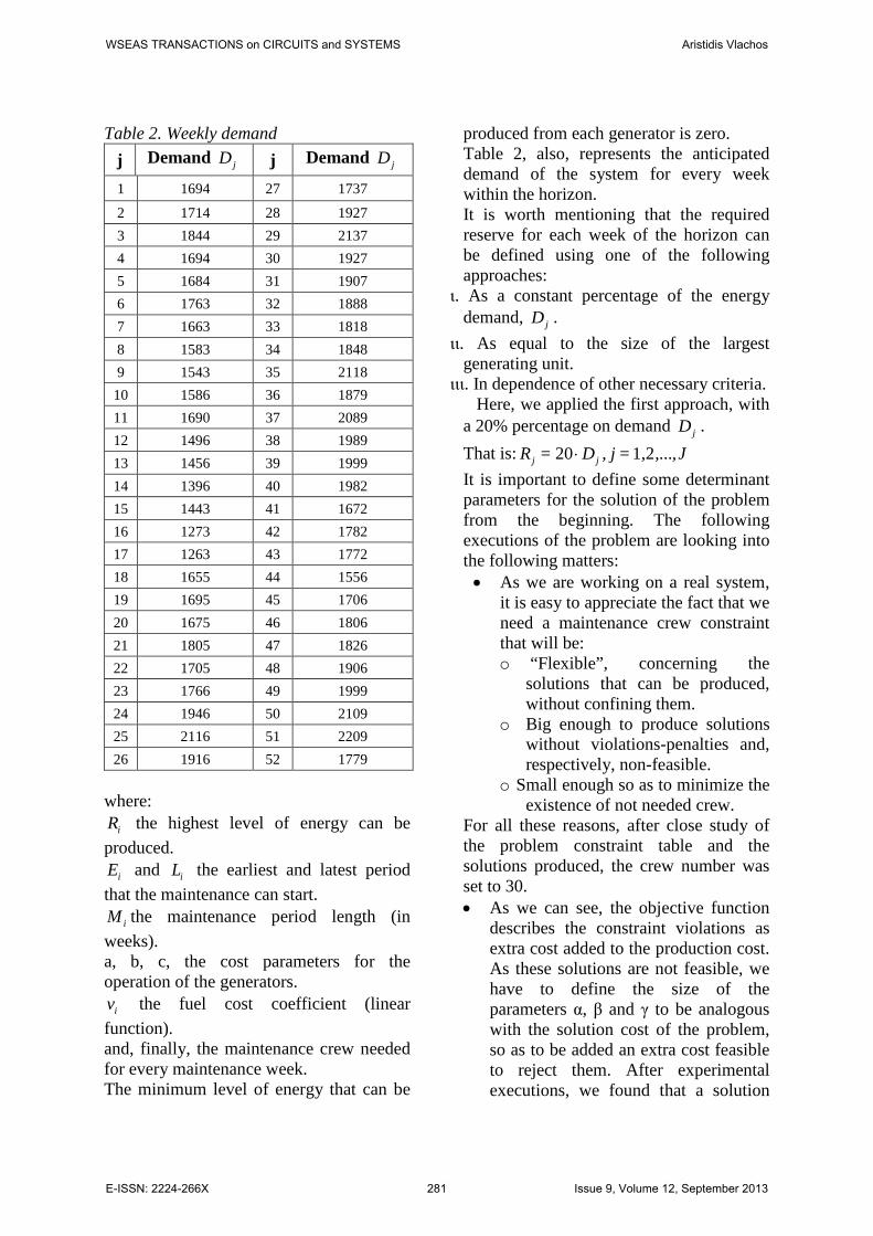
Table 2. Weekly demand j Demand jD j Demand jD

1 1694 27 1737

2 1714 28 1927 3 1844 29 2137 4 1694 30 1927 5 1684 31 1907 6 1763 32 1888 7 1663 33 1818 8 1583 34 1848 9 1543 35 2118

10 1586 36 1879 11 1690 37 2089 12 1496 38 1989 13 1456 39 1999 14 1396 40 1982 15 1443 41 1672 16 1273 42 1782 17 1263 43 1772 18 1655 44 1556 19 1695 45 1706 20 1675 46 1806 21 1805 47 1826 22 1705 48 1906 23 1766 49 1999 24 1946 50 2109 25 2116 51 2209 26 1916 52 1779

where:

iR the highest level of energy can be produced.

iE and iL the earliest and latest period that the maintenance can start.

iM the maintenance period length (in weeks). a, b, c, the cost parameters for the operation of the generators.

iv the fuel cost coefficient (linear function). and, finally, the maintenance crew needed for every maintenance week. The minimum level of energy that can be

produced from each generator is zero. Table 2, also, represents the anticipated demand of the system for every week within the horizon. It is worth mentioning that the required reserve for each week of the horizon can be defined using one of the following approaches:

ι. As a constant percentage of the energy demand, jD .

ιι. As equal to the size of the largest generating unit.

ιιι. In dependence of other necessary criteria. Here, we applied the first approach, with

a 20% percentage on demand jD . That is: 20 1,2 ...j jR = D , j = , ,J⋅ It is important to define some determinant parameters for the solution of the problem from the beginning. The following executions of the problem are looking into the following matters:

• As we are working on a real system, it is easy to appreciate the fact that we need a maintenance crew constraint that will be: o “Flexible”, concerning the

solutions that can be produced, without confining them.

o Big enough to produce solutions without violations-penalties and, respectively, non-feasible.

o Small enough so as to minimize the existence of not needed crew.

For all these reasons, after close study of the problem constraint table and the solutions produced, the crew number was set to 30. • As we can see, the objective function

describes the constraint violations as extra cost added to the production cost. As these solutions are not feasible, we have to define the size of the parameters α, β and γ to be analogous with the solution cost of the problem, so as to be added an extra cost feasible to reject them. After experimental executions, we found that a solution



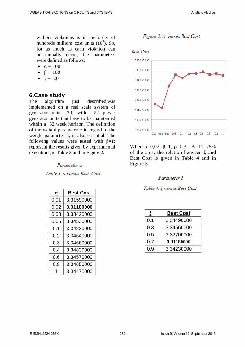
without violations is in the order of hundreds millions cost units (108). So, for as much as each violation can occasionally occur, the parameters were defined as follows: • α = 100 • β = 100 • γ = 20

6.Case study The algorithm just described,was implemented on a real scale system of generator units [20] with 22 power generator units that have to be maintained within a 52 week horizon. The definition of the weight parameter α in regard to the weight parameter β, is also essential. The following values were tested with β=1: represent the results given by experimental executions,in Table 3 and in Figure 2.

α Best Cost 0.01 3.31590000 0.02 3.31180000 0.03 3.33420000 0.05 3.34530000 0.1 3.34230000 0.2 3.34640000 0.3 3.34660000 0.4 3.34830000 0.6 3.34570000 0.8 3.34650000 1 3.34470000

When α=0,02, β=1, ρ=0.3 , Λ=11=25% of the ants, the relation between ξ and Best Cost is given in Table 4 and in Figure 3.

ξ Best Cost

0.1 3.34490000 0.3 3.34560000 0.5 3.32700000 0.7 3.31180000 0.9 3.34230000



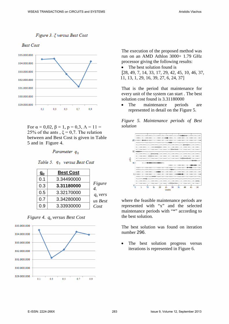
For α = 0,02, β = 1, p = 0,3, Λ = 11 = 25% of the ants , ξ = 0,7. The relation between and Best Cost is given in Table 5 and in Figure 4.

Figure 4.

0q versus Best Cost

Figure 4. 0q versus Best Cost

The execution of the proposed method was run on an AMD Athlon 3000+ 1.79 GHz processor giving the following results: • The best solution found is [28, 49, 7, 14, 33, 17, 29, 42, 45, 10, 46, 37, 11, 13, 1, 29, 16, 39, 27, 6, 24, 37] That is the period that maintenance for every unit of the system can start . The best solution cost found is 3.31180000 • The maintenance periods are

represented in detail on the Figure 5.

Figure 5. Maintenance periods of Best solution

where the feasible maintenance periods are represented with “x” and the selected maintenance periods with “*” according to the best solution. The best solution was found on iteration number 296. • The best solution progress versus

iterations is represented in Figure 6.

qo Best Cost 0.1 3.34490000 0.3 3.31180000 0.5 3.32170000 0.7 3.34280000 0.9 3.33930000



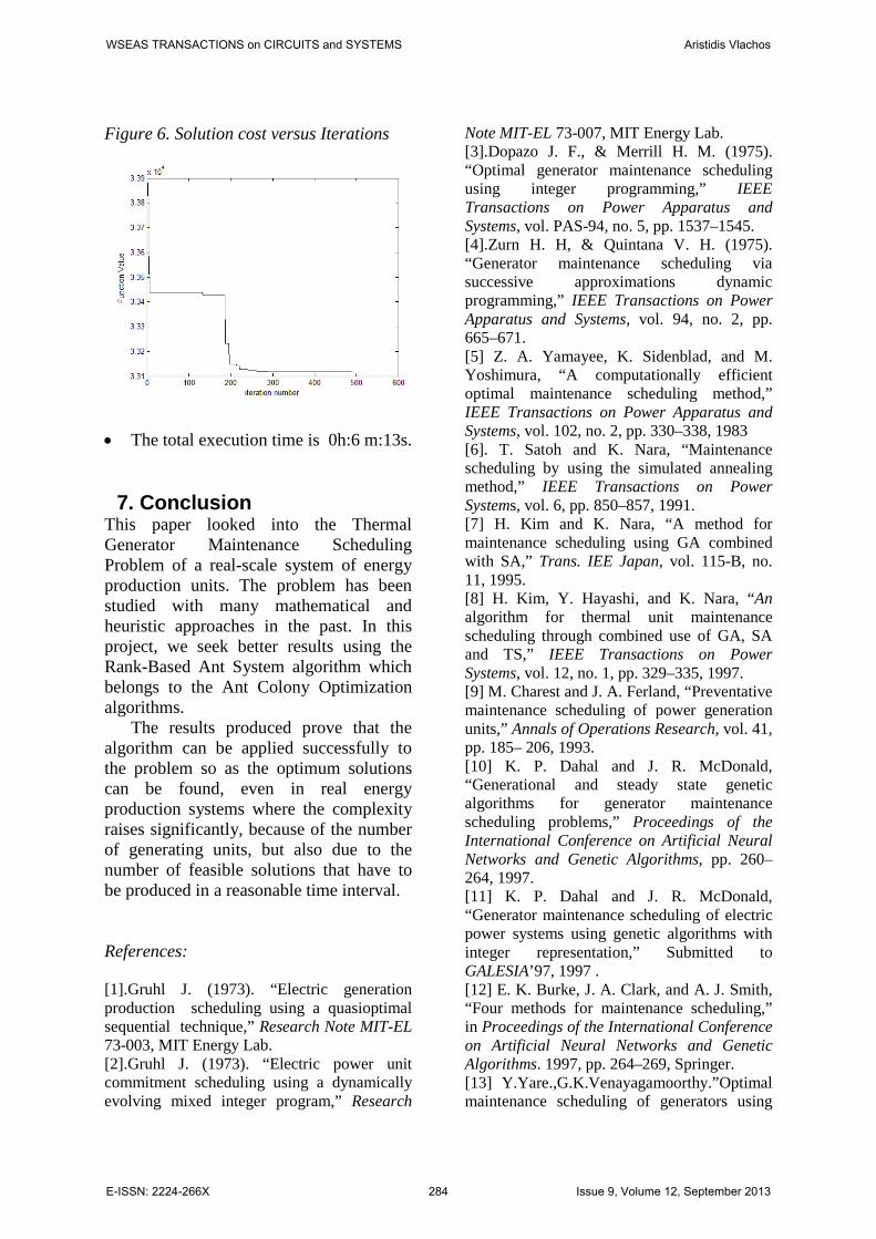
Figure 6. Solution cost versus Iterations

• The total execution time is 0h:6 m:13s.

7. Conclusion

This paper looked into the Thermal Generator Maintenance Scheduling Problem of a real-scale system of energy production units. The problem has been studied with many mathematical and heuristic approaches in the past. In this project, we seek better results using the Rank-Based Ant System algorithm which belongs to the Ant Colony Optimization algorithms.

The results produced prove that the algorithm can be applied successfully to the problem so as the optimum solutions can be found, even in real energy production systems where the complexity raises significantly, because of the number of generating units, but also due to the number of feasible solutions that have to be produced in a reasonable time interval.

References:

[1].Gruhl J. (1973). “Electric generation production scheduling using a quasioptimal sequential technique,” Research Note MIT-EL 73-003, MIT Energy Lab. [2].Gruhl J. (1973). “Electric power unit commitment scheduling using a dynamically evolving mixed integer program,” Research

Note MIT-EL 73-007, MIT Energy Lab. [3].Dopazo J. F., & Merrill H. M. (1975). “Optimal generator maintenance scheduling using integer programming,” IEEE Transactions on Power Apparatus and Systems, vol. PAS-94, no. 5, pp. 1537–1545. [4].Zurn H. H, & Quintana V. H. (1975). “Generator maintenance scheduling via successive approximations dynamic programming,” IEEE Transactions on Power Apparatus and Systems, vol. 94, no. 2, pp. 665–671. [5] Z. A. Yamayee, K. Sidenblad, and M. Yoshimura, “A computationally efficient optimal maintenance scheduling method,” IEEE Transactions on Power Apparatus and Systems, vol. 102, no. 2, pp. 330–338, 1983 [6]. T. Satoh and K. Nara, “Maintenance scheduling by using the simulated annealing method,” IEEE Transactions on Power Systems, vol. 6, pp. 850–857, 1991. [7] H. Kim and K. Nara, “A method for maintenance scheduling using GA combined with SA,” Trans. IEE Japan, vol. 115-B, no. 11, 1995. [8] H. Kim, Y. Hayashi, and K. Nara, “An algorithm for thermal unit maintenance scheduling through combined use of GA, SA and TS,” IEEE Transactions on Power Systems, vol. 12, no. 1, pp. 329–335, 1997. [9] M. Charest and J. A. Ferland, “Preventative maintenance scheduling of power generation units,” Annals of Operations Research, vol. 41, pp. 185– 206, 1993. [10] K. P. Dahal and J. R. McDonald, “Generational and steady state genetic algorithms for generator maintenance scheduling problems,” Proceedings of the International Conference on Artificial Neural Networks and Genetic Algorithms, pp. 260–264, 1997. [11] K. P. Dahal and J. R. McDonald, “Generator maintenance scheduling of electric power systems using genetic algorithms with integer representation,” Submitted to GALESIA’97, 1997 . [12] E. K. Burke, J. A. Clark, and A. J. Smith, “Four methods for maintenance scheduling,” in Proceedings of the International Conference on Artificial Neural Networks and Genetic Algorithms. 1997, pp. 264–269, Springer. [13] Y.Yare.,G.K.Venayagamoorthy.”Optimal maintenance scheduling of generators using



multiple swarms-MDPSO framework”.Egnineering Applications of Artificial Intelligence.23(2010).pp.895-910. [14] J.T.Saraiva,M.L.Pereira,V.T.Mendes,J.C.Sousa.”A simulated Annealing based approach to solve the generator maintenance scheduling problem.Electric Power Systems Research.81(2011).pp.1283-1291. [15].Bullnheimer B., & Hartl R. F., & Strauss C. (1999). A new rank-based version of the ant system: a computational study.Central European Journal for Operations Research and Economics,7(1).pp:25-38. [16].Dorigo M., & Di Caro G., The Ant Colony Optimization Meta-Heuristic, In D.Come, M.Dorigo, and F.Glover, editors, New Ideas in optimization, Mc Graw-Hill.

[17]. Dorigo M., & Gambardella L. M. (1992).

Ant Algorithms for Discrete Optimization, Artificial Life, volume 5, no.2, 137-172.

[18]. Dorigo J. M., & Gambardella L. M. (1997). (2000). Ant colony system:a cooperative learning approach to the Traveling Salesman Problem.IEEE Transaction on Evolutionary computation,1(1),pp:53-66. [19].Bonabeau E. Dorigo M., Theralauz G., 1999 Swarm Intelligence, From Natural to Artificial Systems, a Volume in the Santa Fe Institute Studies in the Sciences of Complexity, Oxford University. [20].Dorigo M and Stutzle T.,Ant Colony Optimization ,The MIT press,2004. [21].Priscila V. S. Z., & Capriles ,Leonardo G.fonseca ,Helio J.C.Barbosa & Afonso C.C.Lemonge. (2007). Rank-based algorithms for truss weight minimization with discrete variables.Communications in numerical methods in engineering ,23,pp:553-575. [22]. Burke E. K., Smith A. J., Hybrid Evolutionary Techniques for the Maintenance Scheduling Problem, IEEE Transactions on Power Systems, 2000, 15(1), pp.1-2. [23] Satoh T., Nara K., Maintenance scheduling by using the simulated annealing method, IEEE Transactions on Power Systems, 1991, 6, p. 850-857. [24] A. J. Wood and B. F. Wood and B. F.

Woolenberg, Power Generation, Operation, and Control, John Wiley, 1984. [25].Ibrahim El-Amin, Salif Duffuaa, Mohammed Abbas, 1998-1999, A tabu search algorithm for maintenance scheduling of generating units, King Fahd University of Petroleum and Minerals.



Rank-Based Ant Colony Algorithm For A Thermal Generator ... · PDF fileRank-Based Ant Colony...

Documents

Transcript of Rank-Based Ant Colony Algorithm For A Thermal Generator ... · PDF fileRank-Based Ant Colony...