ACOUSTIC EMISSION MONITORING OF A WIND …windpower.sandia.gov/asme/AIAA-97-0958.pdf · ACOUSTIC...

1American Institute of Aeronautics and Astronautics

ACOUSTIC EMISSION MONITORING OF A WIND TURBINE BLADE

DURING A FATIGUE TEST∗Ψ

A.G. BeattieDepartment 9742

Sandia National LaboratoryAlbuquerque, NM 87185

∗ This work is supported by the U. S. Department of Energy under Contract DE-AC04-94AL85000.

Ψ This paper is declared a work of the U. S. Government and is not subject to copyright protectionin the United States.

ABSTRACTA fatigue test of a wind turbine blade was conducted

at the National Renewable Energy Laboratory. Acousticemission monitoring of the test was performed, startingwith the second loading level. The acoustic emissiondata showed that this load exceeded the strength of theblade. An oil can type of deformation was seen in twoareas of the upper skin of the blade from the beginningof the second loading. One was near the blade root andthe other was at about 35% of the span. The acousticemission data indicated that no damage was taking placenear the root, but in the deforming area at 35% span,damage occurred from the first cycles of the second load.The test was stopped after approximately one day,although no gross damage had occurred. Several weekslater the test was resumed. Gross damage occurred inapproximately one half hour. The emission data showedevidence of a possible second damage site.

INTRODUCTIONOne of the most common materials used in the

construction of large wind turbine blades is fiberglassreinforced plastic (FRP). A number of failures of suchblades has shown a need for both static and fatiguetesting of new blade designs as well as a betterknowledge of the type and magnitude of real wind loadson the blades. The National Renewable EnergyLaboratory (NREL) has an ongoing program of staticand fatigue load tests on large wind turbine blades. Suchtesting is expensive and can be very time consuming forfatigue tests. Conventional instrumentation on thesetests usually consists of strain gauges. Strainconcentrations in fiber glass blades can be quitelocalized and the number of strain gauges that would beneeded to accurately map out the strain fields on a bladewould be both expensive and complicated. However atest which only determines the static failure load or thenumber of fatigue cycles at a given load and frequency tofailure, while valuable, is only a small part of theinformation which could be obtained. Therefore severalnew methods of instrumentation aimed at acquiring

failure information on critical areas of the blade havebeen tried. These include acoustic emission (AE) andoptical and thermal imaging methods1. This paperdescribes the acoustic emission monitoring of a fatiguetest on a twenty meter blade.

Acoustic emission testing2,3 has been used for yearsto test metallic structures. More recently it has becomethe primary method of testing FRP tanks and structures.Some of the sources of the emission in FRP are matrixcracking, fracture of the matrix-fiber interface andfracture of the fiber. All are present in the failure ofFRP. The two most significant failure mechanisms in awind turbine blade are cracking in the bond between twopieces of the structure, such as a joint between a spar andthe skin, and tears in the skin or a spar. Both involve theprogressive fracture of many fibers. AE has been verysuccessful at detecting all of these failure mechanismsand sometimes identifying them from amplitude analysisof the AE signals. However in large structures, the highacoustic attenuation in FRP precludes amplitude analysisunless the origin of the individual signals can beidentified and corrections for the distances traveledapplied to the signal amplitudes. The usual method oftesting FRP structures has been to apply an array ofsensors spaced so that a moderate amplitude AE signaloccurring midway between them will just barely .triggereach sensor. One then looks at broad areas of damagedefined as the area within the range of each individualsensor. Source location based upon times of signal flightto multiple sensors has seldom been tried on large FRPstructures. Unfortunately, in testing wind turbine blades,one would like a relatively high location accuracy so thatone could determine whether the failure was strictly inthe skin or in the skin-spar bond or a spar failure. In afatigue test, much time could be saved if a region offailure could be identified long before actual failureoccurred. Even when the blade is taken to failure, itwould be extremely valuable to identify other regions,commonly called secondary failure zones, that showeddamage, though of lesser magnitude.

Very little work has been done on AE time of flight


source location or monitoring of fatigue tests of largeFRP structures. Wei and McCarty4 performed fatiguetests on a 7. 5 and a 13 meter wind turbine blade. Theymonitored the AE during static tests between intervals ofat least 10,000 cycles. No monitoring was done duringthe actual fatigue test and only 4 sensors were used in alinear array on the first 20 inches of the blade root.

Working in conjunction with NREL, we have usedAE source location techniques to monitor a static loadtest of a 9 meter blade. The test successfully detectedboth the onset and the location of the failure in real timeand also detected a bond failure between skin and beamwhich was verified when the blade was sectioned. TheFRP skin of this blade had a large frequency dependentattenuation. However, linear AE location wassuccessfully performed by using low frequency (60 KHz)sensors and relatively short intersensor spacings(760mm). Our first attempt to use AE source location onthe surface of a blade during a fatigue test showed thatsource location was possible but not easy. Every sensorsaw a large amount of AE but most of it occurred duringthe maximum rate of load change (rising and falling),not at the peak load. A laboratory study indicated thatmajor damage to the FRP and the resulting AE occurs atthe peak load during the progress of a fatigue test.Therefore, a voltage controlled gate controlled by theload cell signal was used to restrict data acquisition tothe time around the peak load. The time gatingcombined with low frequency sensors and relativelyshort (760mm) sensor spacings did allow AE sourcelocation on the portion of the surface of the bladecovered by the sensor array. Full coverage of bothsurfaces would have required a large number of sensors.Only the critical regions could be covered. With themeasured attenuations and 60 KHz sensors, the area persensor that could be covered using AE source locationwas between 300 and 600 square inches.

TEST DESCRIPTIONThe wind turbine blade in this test was a prototype

of a twenty meter blade. The blade was constructed ofFRP which was bonded to a steel flange at the root. Theblade was mounted horizontally in a flap direction withits root attached to a rigid steel mounting assembly. Theouter 35% of the blade was removed to prevent it fromhitting the roof of the building. The stub was coveredand a hydraulic actuator was attached at the stub end.This actuator was capable of exerting a vertical forceof40% about 28,000 lbs., with a maximum displacementof twenty inches. The actuator was operated sinusoidallyat 0. 75 Hz giving a maximum of 64,800 cycles per day.All tests were run with a positive load only, extendingfrom 10% of peak load to peak load and back.

The acoustic emission was detected with a Physical

Acoustics Corporation (PAC) Spartan AT acousticemission system. This system has 24 data channels.Every channel can measure and record severalparameters for each acoustic emission signal. Parameterscollected in this test were the acoustic emission count,the signal length, the signal rise time, the signal peakamplitude and the area under the signal voltage-timecurve (signal strength or "energy"). The systemmeasures and records the absolute time of signal arrivalat the sensor to within about 0. 25 microseconds andassigns the approximate load at the time of the signal.This load is sampled 100 times per second but assignedto the hit after the data arrives at the main computer.Data pile up can cause the load to be out ofsynchronization with the signal arrival time. Thereforethe "measured" load can be a misleading parameter inthis type of test. This system had the capacity to collect aone gigabyte data file on the hard disk before the datahad to be transferred to storage. Such a file would holdparameters from over 40 million emission signals

PAC R61 sensors were used in this test. Thesesensors have an integral 40 dB preamplifier built intothem, powered from the main system through the signalcable. The peak sensitivity of the sensors is near 60 KHzwith reasonable response to below 30 KHz. The sensorswere applied to the blade with GE Silicone II householdcement, used as both glue and acoustic couplant. Thismaterial is both a good couplant and an excellent gluefor fatigue tests.

The first segment of this test consisted of onemillion cycles at a relatively low peak load. Failure wasnot anticipated at this load so there was no acousticmonitoring of this segment. The load was then increasedby 25%. The blade root region flange was not thought tobe a problem because of extra fiberglass reinforcementaround the first four feet of the blade. One sensor wasplaced on this reinforcement to detect any acousticsignals propagating into the blade from the steelmounting assembly, a problem that had beenencountered in a previous test.

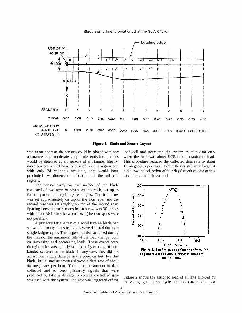
A brief run at the new load showed that an "oilcan" deformation of the upper skin of the blade wastaking place in two areas. The acoustic emission sensorarray was then designed to cover these two areas as wellas the root region just outside of the reinforced region.The complete sensor layout is shown in Figure 1. Sensor24 was placed 60 inches past the top surface array todetect any acoustic signals traveling down the bladefrom the actuator.

The root array consisted of two rows of four sensorseach, one row offset by 45 degrees from the other,covering the region with eight adjacent triangles. Thesensor spacing in a row was 41 inches and the rows were40 inches apart. Because of the high attenuation, this


was as far apart as the sensors could be placed with anyassurance that moderate amplitude emission sourceswould be detected at all sensors of a triangle. Ideally,more sensors would have been used on this region but,with only 24 channels available, that would haveprecluded two-dimensional location in the oil canregions.

The sensor array on the surface of the bladeconsisted of two rows of seven sensors each, set up toform a pattern of adjoining rectangles. The front rowwas set approximately on top of the front spar and thesecond row was set roughly on top of the second spar.Spacing between the sensors in each row was 30 incheswith about 30 inches between rows (the two spars werenot parallel).

A previous fatigue test of a wind turbine blade hadshown that many acoustic signals were detected during asingle fatigue cycle. The largest number occurred duringthe times of the maximum rate of the load change, bothon increasing and decreasing loads. These events werethought to be caused, at least in part, by rubbing of non-bonded surfaces in the blade. In any case, they did notarise from fatigue damage in the previous test. For thisblade, initial measurements showed a data rate of about40 megabytes per hour. To reduce the amount of datacollected and to keep primarily signals that wereproduced by fatigue damage, a voltage controlled gatewas used with the system. The gate was triggered off the

load cell and permitted the system to take data onlywhen the load was above 90% of the maximum load.This procedure reduced the collected data rate to about10 megabytes per hour. While this is still very large, itdid allow the collection of four days' worth of data at thisrate before the disk was full.

Figure 2 shows the assigned load of all hits allowed bythe voltage gate on one cycle. The loads are plotted as a


function of test time. The two located events on thiscycle are given as circled crosses. The approximate loadcurve is shown as a solid line. It is apparent that theassigned loads were close to the actual loads, but boththe quantization errors and some scatter are present.Both located events occur very close to the peak load aswas expected.

SUMMARY OF TEST PROCEDUREThe test proceeded in four stages. In the first stage,

three and a half minutes of data was taken to determinethe initial data rate. Well over an hour of running timewas then used in getting the voltage-controlled gate set.The second stage was to be the start of the main run.This proceeded for an hour and eighteen minutes, atwhich time it was stopped because of problems with theloading equipment. The third stage was started the nextmorning and was continued for 23 hours. It was stoppedbecause the blade surface in one of the oil can regionsappeared to be disintegrating and loud noises wereoccurring on every cycle. The fourth stage was startedseveral weeks later. This test lasted for a total of 36minutes of running time with several stops to examinethe blade. The upper skin in the suspect oil can regionbuckled and pulled away from the front spar. Theloading was stopped and a tear in the skin along theedge of the spar was examined. Loading was restartedand continued for another six minutes when the skinbuckled and tore perpendicular to the spar with apparentdamage to the spar. This ended the test.

DATA ANALYSISIn the analysis of this data, several terms describing

the acoustic emission will be used. An event is thelocalized damage occurring in the blade which producesthe acoustic pulse or burst. A hit is defined when theacoustic burst arrives at and is detected by a sensor. Oneevent usually produces hits on several sensors. An eventis defined by the software when all sensors of a triangleor rectangle are hit within the time it takes an acousticsignal to travel the longest distance between two sensorson the polygon. This time is defined by the acousticvelocity which was roughly measured at 3. 6 mm permicrosecond. Some anisotropy was seen in the velocityand there is always some uncertainty as to which cycle ofthe acoustic signal was detected first. Therefore thistime is increased by about 20% so as to include as manyreal events as possible. Inconsistent data sets (sets withwrong sensors or relative arrival times which did notcorrespond to an event located on the surface) wererejected in the Sandia location calculation. Thedefinition of an event for the root region was that allthree sensors at the comers of a triangle are hit within a400 microsecond span and for the blade, all four sensors

at the comers of a rectangle must be hit within a timespan of 350 microseconds. To be kept as a located event,the calculated location must lie no more than 10%outside of the boundaries of the triangle or rectangle.The Spartan AT location algorithm used a similar logicfor event definition but did not restrict the location towithin the polygon defined by the hit sensors.

Post test analysis of the data was performed by alocation program written at Sandia. This programdirectly read the binary Spartan AT data files. Tocalculate the location, the program used a non-linearleast squares routine. For the blade array, an overdetermined data set was used which included the arrivaltimes from all four corner sensors of the rectangle.While locations could be calculated from only the firstthree sensors hit, this approach produced a very largenumber of located events. Restricting the definition of anevent to four sensors hit, insured that the event wouldhave a large amplitude and relatively low signaldistortion. Experience by many practitioners3 suggeststhat such an event is more likely to be caused by fiberbreakage than lower amplitude sources such as matrixcrazing or rupture of the fiber matrix bond. One morecriteria was applied to the calculated locations. Sincethe data was an over determined set, any errors in thetime measurements would result in a less than perfect fitof the calculated location to the data. The non-linearleast squares fitting program calculates a parameterwhich is an indication of the goodness of the fit. Anydata set which did not produce a reasonable value of thisparameter was discarded. The rejection criteria wasdetermined after extensive experimentation with theprogram on a variety of data sets. There were more thansufficient data points remaining to show just where thedamage was located. At most, discarding these pointswould give an underestimate of the intensity of thedamage. With the magnitude of the damage that wasoccurring in this blade, a small fraction of the totalnumber of emissions is more than capable of definingthe damaged regions.

Examination of the raw data showed many setsfrom individual sensors which had signal rise times ofonly a few microseconds (for this system, the signal risetime is defined as the time between the first detection ofthe signal and the time of occurrence of the peakamplitude). The frequency dependent attenuation offiberglass is such that only very large events will havefrequency components above 100 KHz. Typical acousticemission signals which have propagated from growingflaws will take several cycles of their dominantfrequency to reach their peak amplitude. One cycle of a50 KHz wave lasts 20 microseconds. Therefore, allsignals with rise times less than 20 microseconds weredeclared invalid for source location. This does not mean


that the signals were not real acoustic emission. Whatusually happens is that the system rearms itself to takenew data in the middle of a signal and immediatelytriggers so that the signal actually started before the starttime assigned it by the system. Thus such a signal, whileproduced by real damage, is useless in determining thelocation of the signal source.

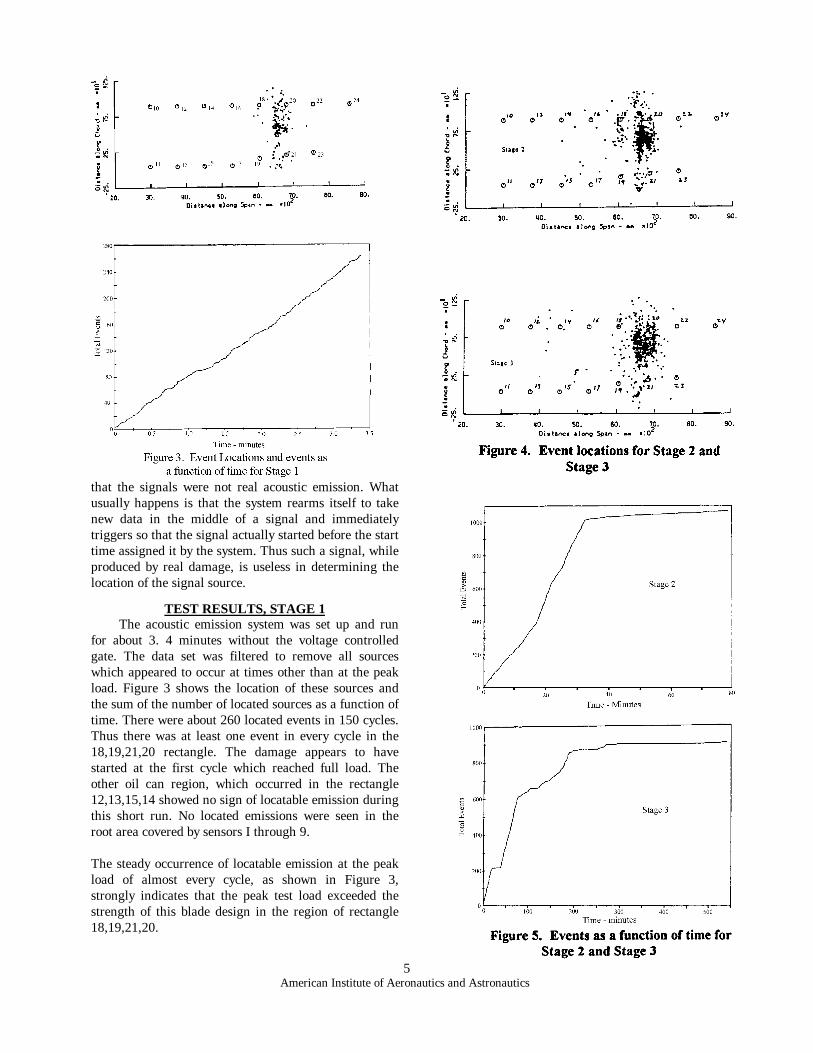
TEST RESULTS, STAGE 1The acoustic emission system was set up and run

for about 3. 4 minutes without the voltage controlledgate. The data set was filtered to remove all sourceswhich appeared to occur at times other than at the peakload. Figure 3 shows the location of these sources andthe sum of the number of located sources as a function oftime. There were about 260 located events in 150 cycles.Thus there was at least one event in every cycle in the18,19,21,20 rectangle. The damage appears to havestarted at the first cycle which reached full load. Theother oil can region, which occurred in the rectangle12,13,15,14 showed no sign of locatable emission duringthis short run. No located emissions were seen in theroot area covered by sensors I through 9.

The steady occurrence of locatable emission at the peakload of almost every cycle, as shown in Figure 3,strongly indicates that the peak test load exceeded thestrength of this blade design in the region of rectangle18,19,21,20.


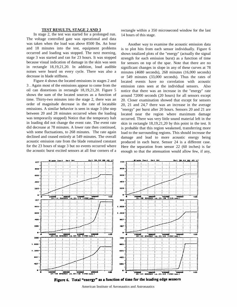
TEST RESULTS, STAGE 2 AND 3In stage 2, the test was started for a prolonged run.

The voltage controlled gate was operational and datawas taken when the load was above 8500 lbs. An hourand 18 minutes into the test, equipment problemsoccurred and loading was stopped. The next morning,stage 3 was started and ran for 23 hours. It was stoppedbecause visual indication of damage in the skin was seenin rectangle 18,19,21,20. In addition, loud audiblenoises were heard on every cycle. There was also adecrease in blade stiffness.

Figure 4 shows the located emissions in stages 2 and3 . Again most of the emissions appear to come from theoil can distortions in rectangle 18,19,21,20. Figure 5shows the sum of the located sources as a function oftime. Thirty-two minutes into the stage 2, there was anorder of magnitude decrease in the rate of locatableemissions. A similar behavior is seen in stage 3 (the stepbetween 20 and 28 minutes occurred when the loadingwas temporarily stopped) Notice that the temporary haltin loading did not change the event rate. The event ratedid decrease at 78 minutes. A lower rate then continued,with some fluctuations, to 268 minutes. The rate againdeclined and ceased entirely at 549 minutes. The overallacoustic emission rate from the blade remained constantfor the 23 hours of stage 3 but no events occurred wherethe acoustic burst excited sensors at all four corners of a

rectangle within a 350 microsecond window for the last14 hours of this stage.

Another way to examine the acoustic emission datais to plot hits from each sensor individually. Figure 6shows totalized plots of the "energy" (actually the signalstrength for each emission burst) as a function of timefor sensors on top of the spar. Note that there are nosignificant changes in slope in any of these curves at 78minutes (4680 seconds), 268 minutes (16,000 seconds)or 549 minutes (33,000 seconds). Thus the rates oflocated events have no correlation with acousticemission rates seen at the individual sensors. Alsonotice that there was an increase in the "energy" ratearound 72000 seconds (20 hours) for all sensors except20. Closer examination showed that except for sensors20, 21 and 24,7 there was an increase in the average"energy" per burst after 20 hours. Sensors 20 and 21 arelocated near the region where maximum damageoccurred. There was very little sound material left in theskin in rectangle 18,19,21,20 by this point in the test. Itis probable that this region weakened, transferring moreload to the surrounding regions. This should increase thedamage and lead to more acoustic energy beingproduced in each burst. Sensor 24 is a different case.Here the separation from sensor 22 (60 inches) is farenough so that the attenuation would allow few, if any,


signals to excite both sensors. The increase here wasmuch larger, proportionally, than that seen in othersensors. The sensor was positioned to tiy to detect anydamage occurring near the loading point on the bladeand such damage is probably what is being seen. Theaverage "energy" per burst decreased for sensor 24beyond the 20 hour point which reinforces theassumption that this is a different mechanism from thatseen in the other sensors.

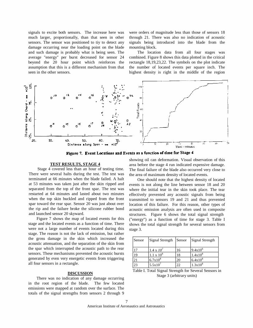
TEST RESULTS, STAGE 4Stage 4 covered less than an hour of testing time.

There were several halts during the test. The test wasterminated at 66 minutes when the blade failed. A haltat 53 minutes was taken just after the skin ripped andseparated from the top of the front spar. The test wasrestarted at 64 minutes and lasted about two minuteswhen the top skin buckled and ripped from the frontspar toward the rear spar. Sensor 20 was just about overthe rip and the failure broke the silicone rubber bondand launched sensor 20 skyward.

Figure 7 shows the map of located events for thisstage and the located events as a function of time. Therewere not a large number of events located during thisstage. The reason is not the lack of emission, but ratherthe gross damage in the skin which increased theacoustic attenuation, and the separation of the skin fromthe spar which interrupted the acoustic path to the rearsensors. These mechanisms prevented the acoustic burstsgenerated by even very energetic events from triggeringall four sensors in a rectangle.

DISCUSSIONThere was no indication of any damage occurring

in the root region of the blade. The few locatedemissions were mapped at random over the surface. Thetotals of the signal strengths from sensors 2 through 9

were orders of magnitude less than those of sensors 18through 21. There was also no indication of acousticsignals being introduced into the blade from themounting block.

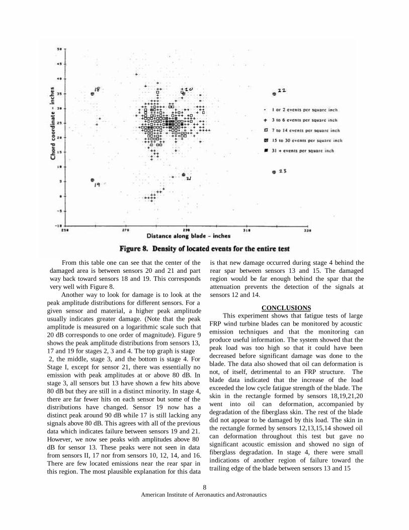
The location data from all four stages wascombined. Figure 8 shows this data plotted in the criticalrectangle 18,19,23,22. The symbols on the plot indicatethe number of located events per square inch. Thehighest density is right in the middle of the region

showing oil can deformation. Visual observation of thisarea before the stage 4 run indicated expensive damage.The final failure of the blade also occurred very close tothe area of maximum density of located events.

One should note that the highest density of locatedevents is not along the line between sensor 18 and 20where the initial tear in the skin took place. The teareffectively prevented any acoustic signals from beingtransmitted to sensors 19 and 21 and thus preventedlocation of this failure. For this reason, other types ofacoustic emission analysis are often used in compositestructures. Figure 6 shows the total signal strength("energy") as a function of time for stage 3. Table Ishows the total signal strength for several sensors fromstage 3.

Sensor Signal Strength Sensor Signal Strength

17 1.4 x 107 16 9.4x106

19 1.1 x 108 18 1.4x108

21 6.7x108 20 6.4x108

23 5.5x107 22 1.3x108

Table I. Total Signal Strength for Several Sensors inStage 3 (arbitrary units)


From this table one can see that the center of thedamaged area is between sensors 20 and 21 and partway back toward sensors 18 and 19. This correspondsvery well with Figure 8.

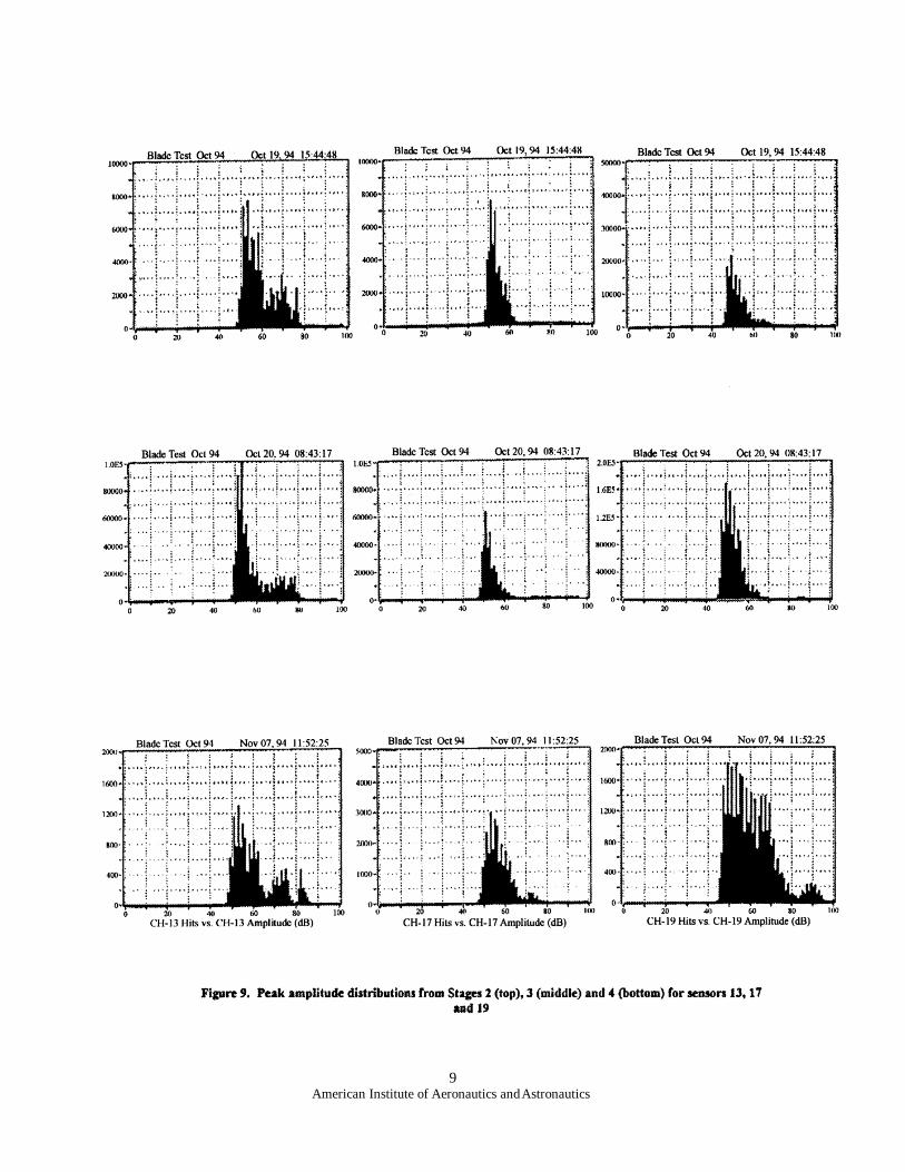
Another way to look for damage is to look at thepeak amplitude distributions for different sensors. For agiven sensor and material, a higher peak amplitudeusually indicates greater damage. (Note that the peakamplitude is measured on a logarithmic scale such that20 dB corresponds to one order of magnitude). Figure 9shows the peak amplitude distributions from sensors 13,17 and 19 for stages 2, 3 and 4. The top graph is stage 2, the middle, stage 3, and the bottom is stage 4. ForStage I, except for sensor 21, there was essentially noemission with peak amplitudes at or above 80 dB. Instage 3, all sensors but 13 have shown a few hits above80 dB but they are still in a distinct minority. In stage 4,there are far fewer hits on each sensor but some of thedistributions have changed. Sensor 19 now has adistinct peak around 90 dB while 17 is still lacking anysignals above 80 dB. This agrees with all of the previousdata which indicates failure between sensors 19 and 21.However, we now see peaks with amplitudes above 80dB for sensor 13. These peaks were not seen in datafrom sensors II, 17 nor from sensors 10, 12, 14, and 16.There are few located emissions near the rear spar inthis region. The most plausible explanation for this data

is that new damage occurred during stage 4 behind therear spar between sensors 13 and 15. The damagedregion would be far enough behind the spar that theattenuation prevents the detection of the signals atsensors 12 and 14.

CONCLUSIONSThis experiment shows that fatigue tests of large

FRP wind turbine blades can be monitored by acousticemission techniques and that the monitoring canproduce useful information. The system showed that thepeak load was too high so that it could have beendecreased before significant damage was done to theblade. The data also showed that oil can deformation isnot, of itself, detrimental to an FRP structure. Theblade data indicated that the increase of the loadexceeded the low cycle fatigue strength of the blade. Theskin in the rectangle formed by sensors 18,19,21,20went into oil can deformation, accompanied bydegradation of the fiberglass skin. The rest of the bladedid not appear to be damaged by this load. The skin inthe rectangle formed by sensors 12,13,15,14 showed oilcan deformation throughout this test but gave nosignificant acoustic emission and showed no sign offiberglass degradation. In stage 4, there were smallindications of another region of failure toward thetrailing edge of the blade between sensors 13 and 15


ACKNOWLEDGEMENTThe author would like to thank Jim Johnson, Mike

Jenks and all the personnel of the NREL wind turbinetesting facility for their valuable help and consultation.He would also like to thank Herb Sutherland of Sandiaand Walt Musial of NREL for a critical review of thisPaper.

REFERENCES1. H. Sutherland, A. Beattie, B. Hansche, W.

Musial, J. Allread, J. Johnson and M. Summers (1994),"The Application of Non-destructive Techniques to theTesting of a Wind Turbine Blade", Sandia NationalLaboratories Report SAND93-1380

2. A. G. Beattie (1983), "Acoustic Emission,Principals and Instrumentation", Journal of AcousticEmission, 2(l-2):95-128

3. ASNT (1987), Nondestructive TestingHandbook, Volume 5, Acoustic Emission Testing, R. K.Miller and PMcIntireed. ASNT

4. J. Wei and J. McCarty (1993), "AcousticEmission Evaluation of Composite Wind Turbine BladesDuring Fatigue Testing", Wind Engineering 17(6):266-274

ACOUSTIC EMISSION MONITORING OF A WIND …windpower.sandia.gov/asme/AIAA-97-0958.pdf · ACOUSTIC...

Documents

Transcript of ACOUSTIC EMISSION MONITORING OF A WIND …windpower.sandia.gov/asme/AIAA-97-0958.pdf · ACOUSTIC...