05 Dynamics
40
Robotics Dynamics 1D point mass, damping & oscillation, PID, dynamics of mechanical systems, Euler-Lagrange equation, Newton-Euler recursion, general robot dynamics, joint space control, reference trajectory following, operational space control Marc Toussaint U Stuttgart
-
Upload
xzax-tornadox -
Category
Documents
-
view
15 -
download
0
description
dynamic
Transcript of 05 Dynamics
Robotics
Dynamics
1D point mass, damping & oscillation, PID,dynamics of mechanical systems,
Euler-Lagrange equation, Newton-Eulerrecursion, general robot dynamics, joint space
control, reference trajectory following,operational space control
Marc ToussaintU Stuttgart
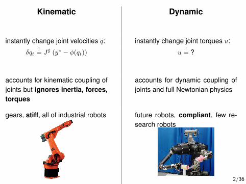
Kinematic Dynamic
instantly change joint velocities q: instantly change joint torques u:
δqt!= J] (y∗ − φ(qt)) u
!= ?
accounts for kinematic coupling ofjoints but ignores inertia, forces,torques
accounts for dynamic coupling ofjoints and full Newtonian physics
gears, stiff, all of industrial robots future robots, compliant, few re-search robots
2/36
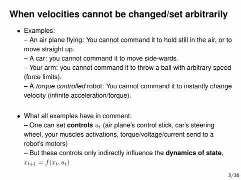
When velocities cannot be changed/set arbitrarily
• Examples:– An air plane flying: You cannot command it to hold still in the air, or tomove straight up.– A car: you cannot command it to move side-wards.– Your arm: you cannot command it to throw a ball with arbitrary speed(force limits).– A torque controlled robot: You cannot command it to instantly changevelocity (infinite acceleration/torque).
• What all examples have in comment:– One can set controls ut (air plane’s control stick, car’s steeringwheel, your muscles activations, torque/voltage/current send to arobot’s motors)– But these controls only indirectly influence the dynamics of state,xt+1 = f(xt, ut)
3/36
Dynamics
• The dynamics of a system describes how the controls ut influence thechange-of-state of the system
xt+1 = f(xt, ut)
– The notation xt refers to the dynamic state of the system: e.g., jointpositions and velocities xt = (qt, qt).– f is an arbitrary function, often smooth
4/36
Outline
• We start by discussing a 1D point mass for 3 reasons:– The most basic force-controlled system with inertia– We can introduce and understand PID control– The behavior of a point mass under PID control is a reference that we can
also follow with arbitrary dynamic robots (if the dynamics are known)
• We discuss computing the dynamics of general robotic systems– Euler-Lagrange equations– Euler-Newton method
• We derive the dynamic equivalent of inverse kinematics:– operational space control
5/36
PID and a 1D point mass
6/36
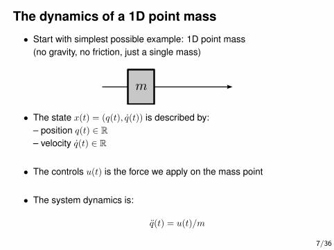
The dynamics of a 1D point mass
• Start with simplest possible example: 1D point mass(no gravity, no friction, just a single mass)
• The state x(t) = (q(t), q(t)) is described by:– position q(t) ∈ R– velocity q(t) ∈ R
• The controls u(t) is the force we apply on the mass point
• The system dynamics is:
q(t) = u(t)/m
7/36
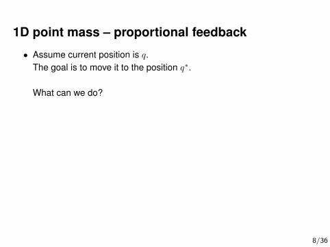
1D point mass – proportional feedback
• Assume current position is q.The goal is to move it to the position q∗.
What can we do?
• Idea 1:“Always pull the mass towards the goal q∗:”
u = Kp (q∗ − q)
8/36
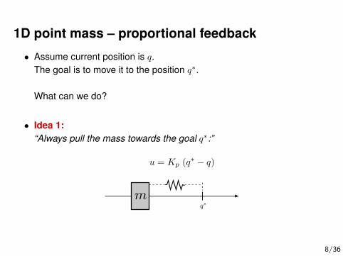
1D point mass – proportional feedback
• Assume current position is q.The goal is to move it to the position q∗.
What can we do?
• Idea 1:“Always pull the mass towards the goal q∗:”
u = Kp (q∗ − q)
8/36
1D point mass – proportional feedback
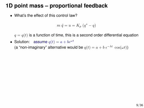
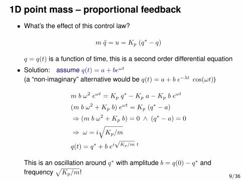
• What’s the effect of this control law?
m q = u = Kp (q∗ − q)
q = q(t) is a function of time, this is a second order differential equation
• Solution: assume q(t) = a+ beωt
(a “non-imaginary” alternative would be q(t) = a+ b ε−λt cos(ωt))
m b ω2 eωt = Kp q∗ −Kp a−Kp b e
ωt
(m b ω2 +Kp b) eωt = Kp (q∗ − a)
⇒ (m b ω2 +Kp b) = 0 ∧ (q∗ − a) = 0
⇒ ω = i√Kp/m
q(t) = q∗ + b ei√Kp/m t
This is an oscillation around q∗ with amplitude b = q(0)− q∗ andfrequency
√Kp/m!
9/36
1D point mass – proportional feedback
• What’s the effect of this control law?
m q = u = Kp (q∗ − q)
q = q(t) is a function of time, this is a second order differential equation
• Solution: assume q(t) = a+ beωt
(a “non-imaginary” alternative would be q(t) = a+ b ε−λt cos(ωt))
m b ω2 eωt = Kp q∗ −Kp a−Kp b e
ωt
(m b ω2 +Kp b) eωt = Kp (q∗ − a)
⇒ (m b ω2 +Kp b) = 0 ∧ (q∗ − a) = 0
⇒ ω = i√Kp/m
q(t) = q∗ + b ei√Kp/m t
This is an oscillation around q∗ with amplitude b = q(0)− q∗ andfrequency
√Kp/m!
9/36
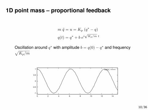
1D point mass – proportional feedback
m q = u = Kp (q∗ − q)
q(t) = q∗ + b ei√Kp/m t
Oscillation around q∗ with amplitude b = q(0)− q∗ and frequency√Kp/m
-1
-0.5
0
0.5
1
0 2 4 6 8 10 12 14
cos(x)
10/36
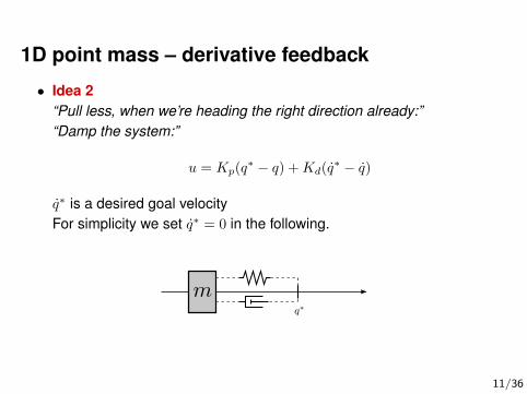
1D point mass – derivative feedback
• Idea 2“Pull less, when we’re heading the right direction already:”“Damp the system:”
u = Kp(q∗ − q) +Kd(q
∗ − q)
q∗ is a desired goal velocityFor simplicity we set q∗ = 0 in the following.
11/36
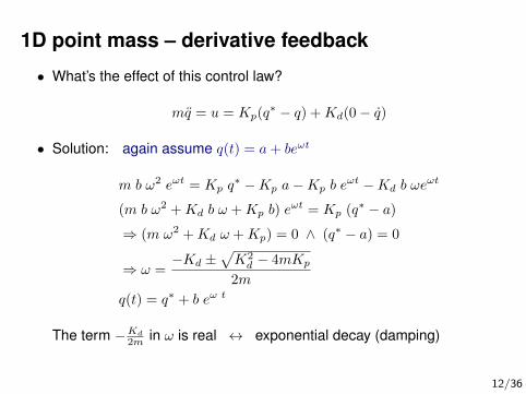
1D point mass – derivative feedback
• What’s the effect of this control law?
mq = u = Kp(q∗ − q) +Kd(0− q)
• Solution: again assume q(t) = a+ beωt
m b ω2 eωt = Kp q∗ −Kp a−Kp b e
ωt −Kd b ωeωt
(m b ω2 +Kd b ω +Kp b) eωt = Kp (q∗ − a)
⇒ (m ω2 +Kd ω +Kp) = 0 ∧ (q∗ − a) = 0
⇒ ω =−Kd ±
√K2d − 4mKp
2m
q(t) = q∗ + b eω t
The term −Kd
2m in ω is real ↔ exponential decay (damping)
12/36
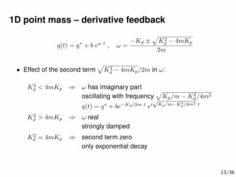
1D point mass – derivative feedback
q(t) = q∗ + b eω t , ω =−Kd ±
√K2d − 4mKp
2m
• Effect of the second term√K2d − 4mKp/2m in ω:
K2d < 4mKp ⇒ ω has imaginary part
oscillating with frequency√Kp/m−K2
d/4m2
q(t) = q∗ + be−Kd/2m t ei√Kp/m−K2
d/4m2 t
K2d > 4mKp ⇒ ω real
strongly damped
K2d = 4mKp ⇒ second term zero
only exponential decay
13/36
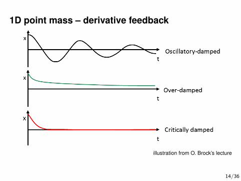
1D point mass – derivative feedback
illustration from O. Brock’s lecture
14/36
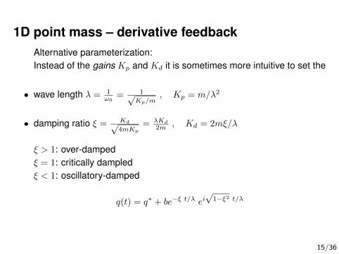
1D point mass – derivative feedbackAlternative parameterization:Instead of the gains Kp and Kd it is sometimes more intuitive to set the
• wave length λ = 1ω0
= 1√Kp/m
, Kp = m/λ2
• damping ratio ξ = Kd√4mKp
= λKd
2m , Kd = 2mξ/λ
ξ > 1: over-dampedξ = 1: critically dampledξ < 1: oscillatory-damped
q(t) = q∗ + be−ξ t/λ ei√
1−ξ2 t/λ
15/36
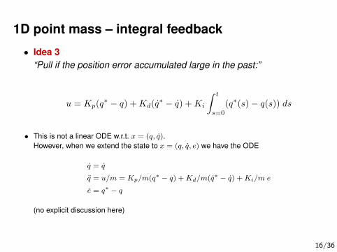
1D point mass – integral feedback
• Idea 3“Pull if the position error accumulated large in the past:”
u = Kp(q∗ − q) +Kd(q
∗ − q) +Ki
∫ t
s=0
(q∗(s)− q(s)) ds
• This is not a linear ODE w.r.t. x = (q, q).However, when we extend the state to x = (q, q, e) we have the ODE
q = q
q = u/m = Kp/m(q∗ − q) +Kd/m(q∗ − q) +Ki/m e
e = q∗ − q
(no explicit discussion here)
16/36
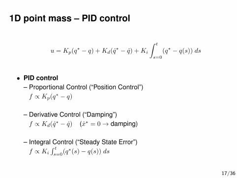
1D point mass – PID control
u = Kp(q∗ − q) +Kd(q
∗ − q) +Ki
∫ t
s=0
(q∗ − q(s)) ds
• PID control– Proportional Control (“Position Control”)f ∝ Kp(q
∗ − q)
– Derivative Control (“Damping”)f ∝ Kd(q
∗ − q) (x∗ = 0→ damping)
– Integral Control (“Steady State Error”)f ∝ Ki
∫ ts=0
(q∗(s)− q(s)) ds
17/36
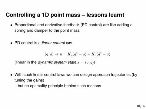
Controlling a 1D point mass – lessons learnt
• Proportional and derivative feedback (PD control) are like adding aspring and damper to the point mass
• PD control is a linear control law
(q, q) 7→ u = Kp(q∗ − q) +Kd(q
∗ − q)
(linear in the dynamic system state x = (q, q))
• With such linear control laws we can design approach trajectories (bytuning the gains)– but no optimality principle behind such motions
18/36
Dynamics of mechanical systems
19/36
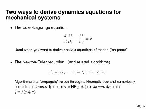
Two ways to derive dynamics equations formechanical systems
• The Euler-Lagrange equation
d
dt
∂L
∂q− ∂L
∂q= u
Used when you want to derive analytic equations of motion (“on paper”)
• The Newton-Euler recursion (and related algorithms)
fi = mvi , ui = Iiw + w × Iw
Algorithms that “propagate” forces through a kinematic tree and numericallycompute the inverse dynamics u = NE(q, q, q) or forward dynamicsq = f(q, q, u).
20/36
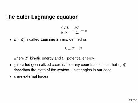
The Euler-Lagrange equation
d
dt
∂L
∂q− ∂L
∂q= u
• L(q, q) is called Lagrangian and defined as
L = T − U
where T=kinetic energy and U=potential energy.
• q is called generalized coordinate – any coordinates such that (q, q)
describes the state of the system. Joint angles in our case.
• u are external forces
21/36
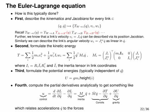
The Euler-Lagrange equation• How is this typically done?• First, describe the kinematics and Jacobians for every link i:
(q, q) 7→ {TW→i(q), vi, wi}
Recall TW→i(q) = TW→A TA→A′ (q) TA′→B TB→B′ (q) · · ·Further, we know that a link’s velocity vi = Jiq can be described via its position Jacobian.Similarly we can describe the link’s angular velocity wi = Jw
i q as linear in q.
• Second, formulate the kinetic energy
T =∑i
1
2miv
2i +
1
2w>i Iiwi =
∑i
1
2q>Miq , Mi =
JiJwi
>miI3 0
0 Ii
JiJwi
where Ii = RiIiR>i and Ii the inertia tensor in link coordinates
• Third, formulate the potential energies (typically independent of q)
U = gmiheight(i)
• Fourth, compute the partial derivatives analytically to get something like
u︸︷︷︸control
=d
dt
∂L
∂q− ∂L
∂q= M︸︷︷︸
inertia
q + Mq − ∂T
∂q︸ ︷︷ ︸Coriolis
+∂U
∂q︸︷︷︸gravity
which relates accelerations q to the forces 22/36
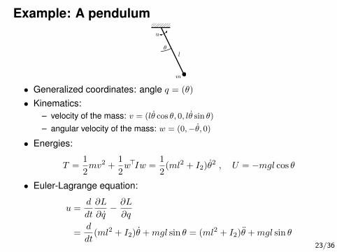
Example: A pendulum
• Generalized coordinates: angle q = (θ)
• Kinematics:– velocity of the mass: v = (lθ cos θ, 0, lθ sin θ)
– angular velocity of the mass: w = (0,−θ, 0)
• Energies:
T =1
2mv2 +
1
2w>Iw =
1
2(ml2 + I2)θ2 , U = −mgl cos θ
• Euler-Lagrange equation:
u =d
dt
∂L
∂q− ∂L
∂q
=d
dt(ml2 + I2)θ +mgl sin θ = (ml2 + I2)θ +mgl sin θ
23/36
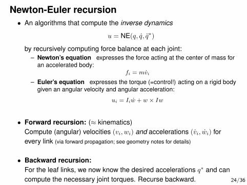
Newton-Euler recursion• An algorithms that compute the inverse dynamics
u = NE(q, q, q∗)
by recursively computing force balance at each joint:– Newton’s equation expresses the force acting at the center of mass for
an accelerated body:fi = mvi
– Euler’s equation expresses the torque (=control!) acting on a rigid bodygiven an angular velocity and angular acceleration:
ui = Iiw + w × Iw
• Forward recursion: (≈ kinematics)Compute (angular) velocities (vi, wi) and accelerations (vi, wi) forevery link (via forward propagation; see geometry notes for details)
• Backward recursion:For the leaf links, we now know the desired accelerations q∗ and cancompute the necessary joint torques. Recurse backward. 24/36
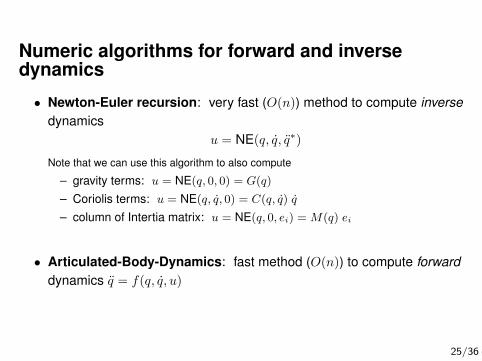
Numeric algorithms for forward and inversedynamics
• Newton-Euler recursion: very fast (O(n)) method to compute inversedynamics
u = NE(q, q, q∗)
Note that we can use this algorithm to also compute
– gravity terms: u = NE(q, 0, 0) = G(q)
– Coriolis terms: u = NE(q, q, 0) = C(q, q) q
– column of Intertia matrix: u = NE(q, 0, ei) = M(q) ei
• Articulated-Body-Dynamics: fast method (O(n)) to compute forwarddynamics q = f(q, q, u)
25/36
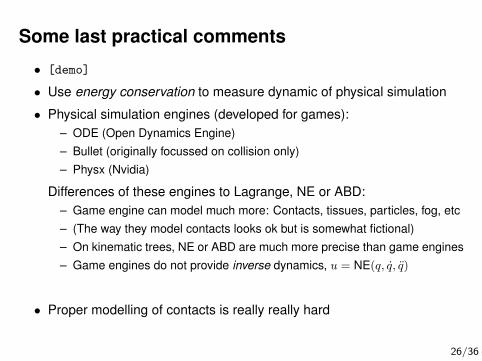
Some last practical comments
• [demo]
• Use energy conservation to measure dynamic of physical simulation
• Physical simulation engines (developed for games):– ODE (Open Dynamics Engine)– Bullet (originally focussed on collision only)– Physx (Nvidia)
Differences of these engines to Lagrange, NE or ABD:– Game engine can model much more: Contacts, tissues, particles, fog, etc– (The way they model contacts looks ok but is somewhat fictional)– On kinematic trees, NE or ABD are much more precise than game engines– Game engines do not provide inverse dynamics, u = NE(q, q, q)
• Proper modelling of contacts is really really hard
26/36
Dynamic control of a robot
27/36
• We previously learnt the effect of PID control on a 1D point mass
• Robots are not a 1D point mass– Neither is each joint a 1D point mass– Applying separate PD control in each joint neglects force coupling
(Poor solution: Apply very high gains separately in each joint↔ makejoints stiff, as with gears.)
• However, knowing the robot dynamics we can transfer ourunderstanding of PID control of a point mass to general systems
28/36
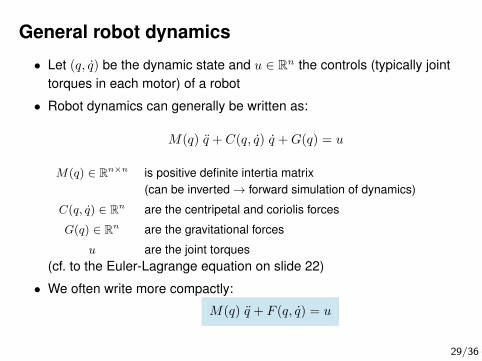
General robot dynamics
• Let (q, q) be the dynamic state and u ∈ Rn the controls (typically jointtorques in each motor) of a robot
• Robot dynamics can generally be written as:
M(q) q + C(q, q) q +G(q) = u
M(q) ∈ Rn×n is positive definite intertia matrix(can be inverted→ forward simulation of dynamics)
C(q, q) ∈ Rn are the centripetal and coriolis forces
G(q) ∈ Rn are the gravitational forces
u are the joint torques(cf. to the Euler-Lagrange equation on slide 22)
• We often write more compactly:
M(q) q + F (q, q) = u
29/36
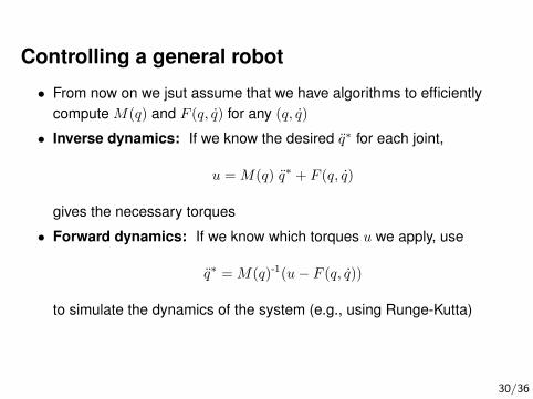
Controlling a general robot
• From now on we jsut assume that we have algorithms to efficientlycompute M(q) and F (q, q) for any (q, q)
• Inverse dynamics: If we know the desired q∗ for each joint,
u = M(q) q∗ + F (q, q)
gives the necessary torques
• Forward dynamics: If we know which torques u we apply, use
q∗ = M(q)-1(u− F (q, q))
to simulate the dynamics of the system (e.g., using Runge-Kutta)
30/36
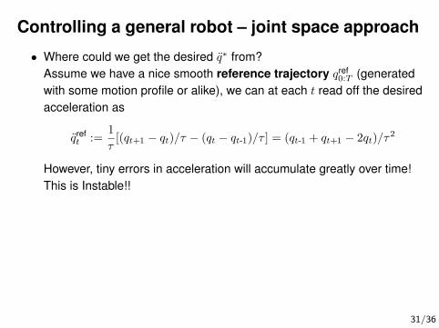
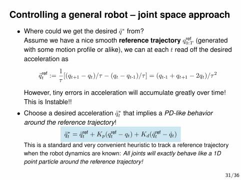
Controlling a general robot – joint space approach
• Where could we get the desired q∗ from?Assume we have a nice smooth reference trajectory qref
0:T (generatedwith some motion profile or alike), we can at each t read off the desiredacceleration as
qreft :=
1
τ[(qt+1 − qt)/τ − (qt − qt-1)/τ ] = (qt-1 + qt+1 − 2qt)/τ
2
However, tiny errors in acceleration will accumulate greatly over time!This is Instable!!
• Choose a desired acceleration q∗t that implies a PD-like behavioraround the reference trajectory!
q∗t = qreft +Kp(q
reft − qt) +Kd(q
reft − qt)
This is a standard and very convenient heuristic to track a reference trajectorywhen the robot dynamics are known: All joints will exactly behave like a 1Dpoint particle around the reference trajectory!
31/36
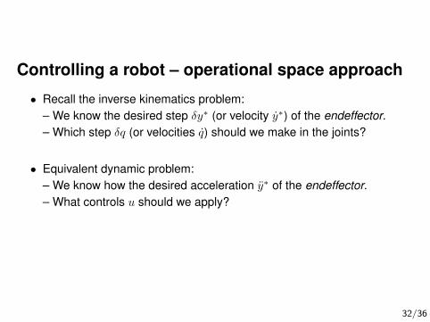
Controlling a robot – operational space approach
• Recall the inverse kinematics problem:– We know the desired step δy∗ (or velocity y∗) of the endeffector.– Which step δq (or velocities q) should we make in the joints?
• Equivalent dynamic problem:– We know how the desired acceleration y∗ of the endeffector.– What controls u should we apply?
32/36
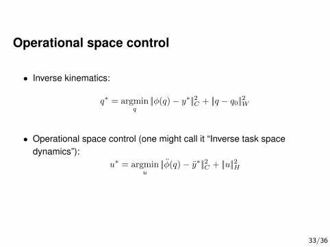
Operational space control
• Inverse kinematics:
q∗ = argminq||φ(q)− y∗||2C + ||q − q0||2W
• Operational space control (one might call it “Inverse task spacedynamics”):
u∗ = argminu||φ(q)− y∗||2C + ||u||2H
33/36
Operational space control
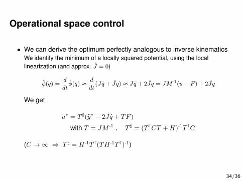
• We can derive the optimum perfectly analogous to inverse kinematicsWe identify the minimum of a locally squared potential, using the locallinearization (and approx. J = 0)
φ(q) =d
dtφ(q) ≈ d
dt(Jq + Jq) ≈ Jq + 2J q = JM -1(u− F ) + 2J q
We get
u∗ = T ](y∗ − 2J q + TF )
with T = JM -1 , T ] = (T>CT +H)-1T>C
(C →∞ ⇒ T ] = H -1T>(TH -1T>)-1)
34/36
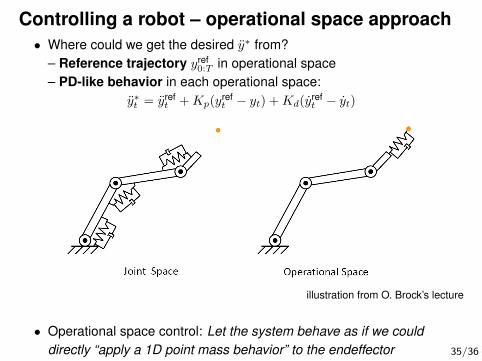
Controlling a robot – operational space approach• Where could we get the desired y∗ from?
– Reference trajectory yref0:T in operational space
– PD-like behavior in each operational space:y∗t = yref
t +Kp(yreft − yt) +Kd(y
reft − yt)
illustration from O. Brock’s lecture
• Operational space control: Let the system behave as if we coulddirectly “apply a 1D point mass behavior” to the endeffector 35/36
Multiple tasks
• Recall trick last time: we defined a “big kinematic map” Φ(q) such that
q∗ = argminq||q − q0||2W + ||Φ(q)||2
• Works analogously in the dynamic case:
u∗ = argminu||u||2H + ||Φ(q)||2
36/36