Angular Momentum

Angular Momentum About Spin Axis

Ω

𝜙

r

rAM (per unit mass) = velocity × moment arm

M = (r? + u)r?

r? = a cos

(f +

¯)v = f (1 Ro)v 0

Ro = ¯/f ! 1

h gH 0

t

2a2

0h

1/2

max

(H 0t

0h)

5/2

3a

Thin-shell approximation: take distance from any point in atmosphere to planet’s barycenterequal to constant radius a

Length of Day

Year

ΔL

OD

(m

s)

1965 1975 1985 1995 2005 2015−2

0

2

4

Year

ΔL

OD

(m

s)

2010 2012 2014

−1

0

1

2

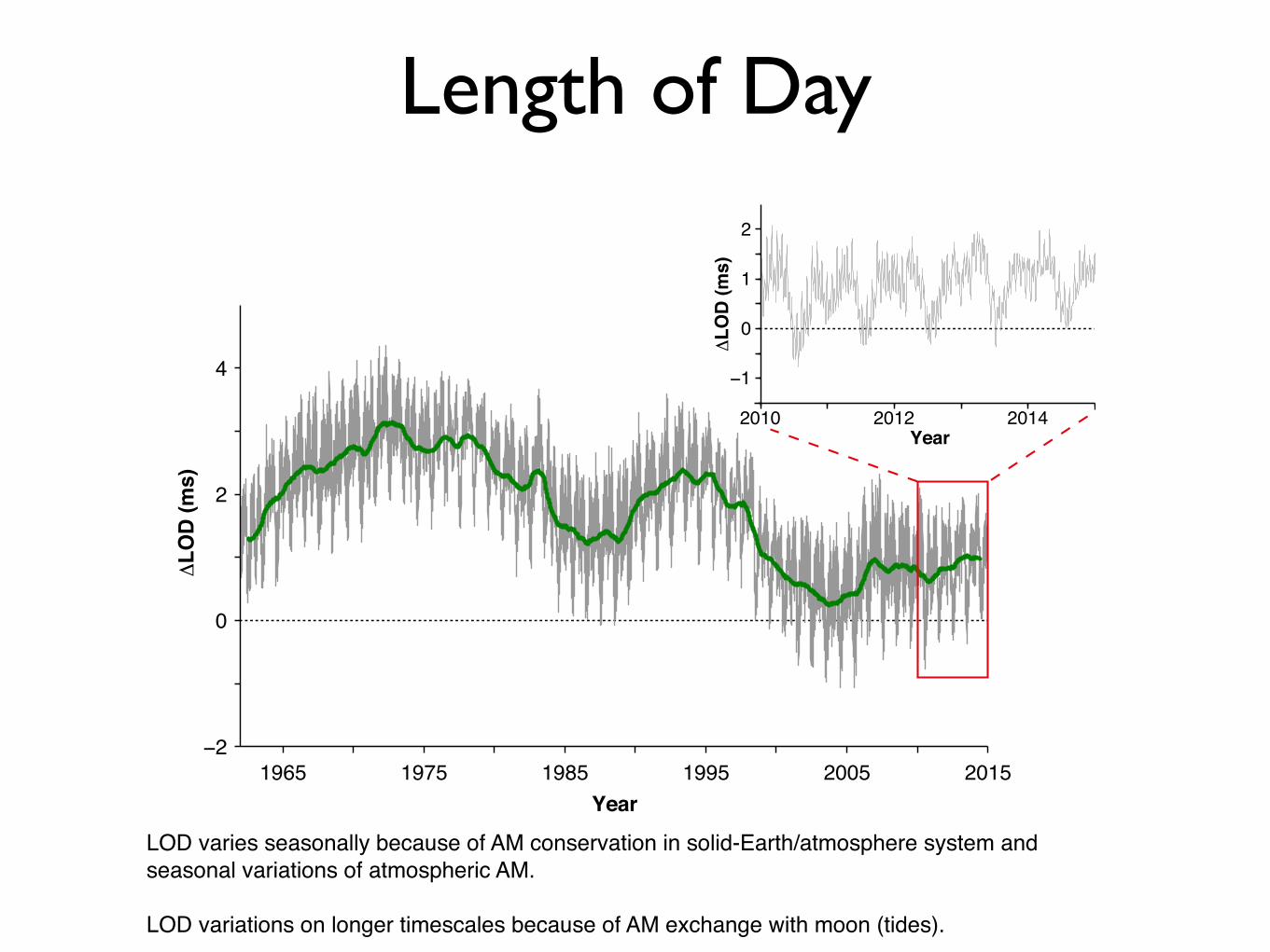
LOD varies seasonally because of AM conservation in solid-Earth/atmosphere system and seasonal variations of atmospheric AM.

LOD variations on longer timescales because of AM exchange with moon (tides).

Angular Momentum in Atmosphere

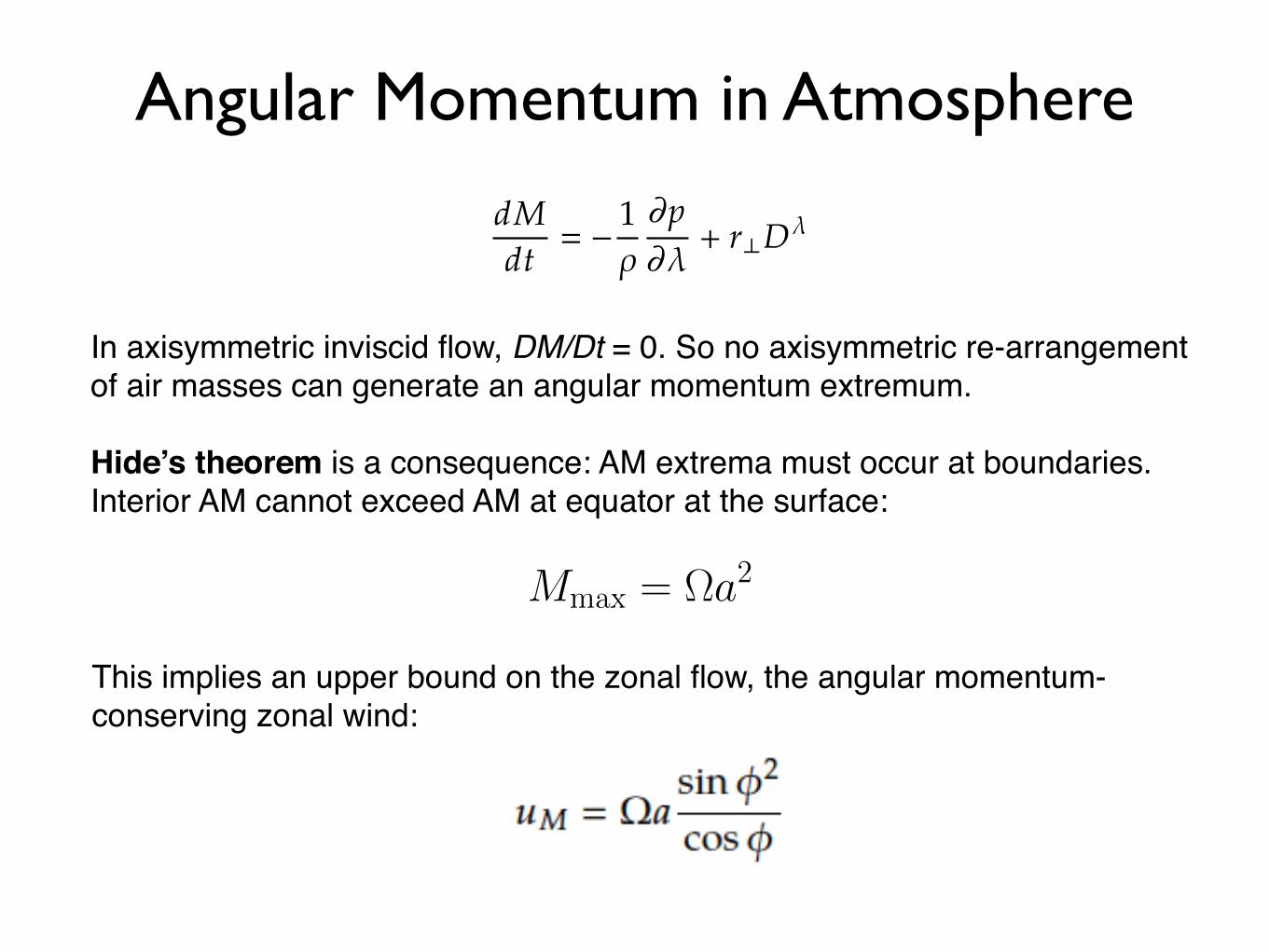
In axisymmetric inviscid flow, DM/Dt = 0. So no axisymmetric re-arrangement of air masses can generate an angular momentum extremum.

Hide’s theorem is a consequence: AM extrema must occur at boundaries. Interior AM cannot exceed AM at equator at the surface:

M = (r? + u)r?

r? = a cos

Mmax

= a2

(f +

¯)v = f (1 Ro)v 0

Ro = ¯/f ! 1

h gH 0

t

2a2

0h

1/2

max

(H 0t

0h)

5/2

3a

This implies an upper bound on the zonal flow, the angular momentum-conserving zonal wind:

FUNDAMENTAL LAWS AND SCALES

GCA_Book December 3, 2014 6x9

15

no gravitational acceleration in the zonal direction. The inertial-frame acceler-ations can then be specied as

dMdt

1@p@

+ r?D . (1.22)

No r? multiplies the pressure derivative here, because the azimuthal compo-nent of the pressure gradient in spherical coordinates, r1

? @, contains an r?factor in the denominator, which cancels the r? factor from the moment arm(see Appendix B).

We can expand this further by substituting the denition of the specic an-gular momentum and expanding the material derivative. Since the only explic-itly time-dependent term is the zonal velocity u in Mu ur?, we obtain

r?@t u + u ·rM + u ·rMu 1@p@

+ r?D . (1.23)

On the left-hand side, the rst term represents the local rate of increase @t Muof the relative angular momentum Mu , associated with local acceleration @t u ofthe zonal ow u. The second term represents the advection of planetary angularmomentum M, and the third term advection of relative angular momentumMu . The advection of planetary angular momentum we can unpack further asu · rM u · r(r2

?) 2u · r? by the same manipulations that lead tothe centrifugal potential (1.15). This we recognize as being proportional to thezonal component of the Coriolis acceleration,

u ·rM 2r?( u) · e . (1.24)

Thus, the advection of planetary angular momentum M by the atmosphericow u represents the Coriolis torque per unit mass in the zonal direction.

The equation (1.23) for the angular momentum component about the spinaxis is an equation for local accelerations @t u of the zonal ow. On the onehand, it can be used to relate such local accelerations to advection of planetaryand relative angular momentum about the spin axis (second and third term onthe left-hand side), and to pressure gradients and drag (right-hand side). Onthe other hand, if zonal ow accelerations can be neglected (e.g., in a statisticallysteady state in the mean), it relates the advection of angular momentum aboutthe spin axis to pressure gradients and drag. We will use it in both ways in thefollowing chapters. We will also use it in the ux form

r?@t (u) + r · u(M + Mu ) @p@

+ r?D , (1.25)

which is more convenient for averaging than the advective form.

1.7.2 Angular Momentum Perpendicular to Spin Axis

The second angular momentum component of interest to us is the componentaround an axis perpendicular to the spin axis, N L · e?, where e? is a unit

AM and Hadley cell

20 60 100140 220 300

AM-conserving zonal wind (m s-1)

15°N 30°N 45°N 60°N 75°N 90°N0°

Latitude

30

20

10

−10

11090 70

40 20 −10−30

30

20

10

−10

11090 70

40 20 −10−30

15°N 30°N 45°N 60°N 75°N 90°N0°

Latitude

100

200

300

500

800

1000Streamfunction (Sv)

100

200

300

500

800

1000

Pres

sure

(hPa

)

Zonal wind (m s-1)

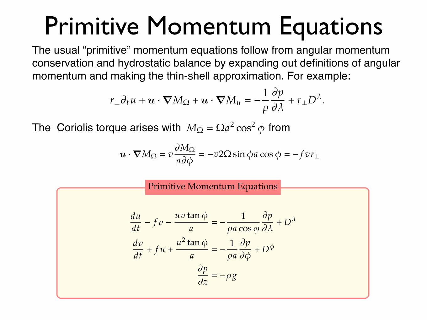
Primitive Momentum EquationsThe usual “primitive” momentum equations follow from angular momentum conservation and hydrostatic balance by expanding out definitions of angular momentum and making the thin-shell approximation. For example:

The Coriolis torque arises with from

16


CHAPTER 1

vector perpendicular to the spin axis, in the equatorial plane, which rotates withthe planet around its spin axis. This angular momentum component involvesow along meridians. It has no planetary component. It is the specic angularmomentum N (r u) · e? obtained by multiplying the moment arm r? bythe meridional velocity v, dened to be positive for northward ow:

N vr?.

To transform the material derivative of the angular momentum componentperpendicular to the spin axis from the inertial reference frame to the rotatingreference frame, the transformation rule (1.20) needs to applied,

da (Ne?)dt

d(Ne?)

dt+ Ne?.

1.8 SCALES AND NONDIMENSIONALIZATION

1.9 HYDROSTATIC BALANCE

1.10 THIN-ATMOSPHERE APPROXIMATION

In the thin atmosphere approximation, we approximate the distance r from anypoint in the atmosphere to the planet’s center by the constant a, the mean radiusof the planet. In approximating equations of motion, we generally want the ap-proximate equations to preserve important physical principles in approximateform. For example, we want the approximate equations to possess a balanceequation for angular momentum, which reduces to a conservation law whenangular momentum is conserved (no torques act on the ow). To ensure thatthis is the case, we start with approximating angular momentum by settingr? r cos a cos for the moment arm. The specic angular momentumcomponent about the spin axis then becomes M M + Mu with

M a2 cos2 and Mu ua cos. (1.26)

The specic angular momentum component about the equatorial plane becomes

N (1.27)

Coriolis torque

u ·rM v@Ma@

v2 sina cos f vr? (1.28)

with Coriolis parameter f 2 sin.4

16


CHAPTER 1

vector perpendicular to the spin axis, in the equatorial plane, which rotates withthe planet around its spin axis. This angular momentum component involvesow along meridians. It has no planetary component. It is the specic angularmomentum N (r u) · e? obtained by multiplying the moment arm r? bythe meridional velocity v, dened to be positive for northward ow:

N vr?.

To transform the material derivative of the angular momentum componentperpendicular to the spin axis from the inertial reference frame to the rotatingreference frame, the transformation rule (1.20) needs to applied,

da (Ne?)dt

d(Ne?)

dt+ Ne?.

1.8 SCALES AND NONDIMENSIONALIZATION

1.9 HYDROSTATIC BALANCE

1.10 THIN-ATMOSPHERE APPROXIMATION

In the thin atmosphere approximation, we approximate the distance r from anypoint in the atmosphere to the planet’s center by the constant a, the mean radiusof the planet. In approximating equations of motion, we generally want the ap-proximate equations to preserve important physical principles in approximateform. For example, we want the approximate equations to possess a balanceequation for angular momentum, which reduces to a conservation law whenangular momentum is conserved (no torques act on the ow). To ensure thatthis is the case, we start with approximating angular momentum by settingr? r cos a cos for the moment arm. The specic angular momentumcomponent about the spin axis then becomes M M + Mu with

M a2 cos2 and Mu ua cos. (1.26)

The specic angular momentum component about the equatorial plane becomes

N (1.27)

Coriolis torque

u ·rM v@Ma@

v2 sina cos f vr? (1.28)

with Coriolis parameter f 2 sin.4



17

dudt f v uv tan

a 1a cos

@p@

+ D

dvdt

+ f u +u2 tan

a 1a@p@

+ D

@p@z

g

Primitive Momentum Equations

1.11 GEOSTROPHIC BALANCE

1.12 THERMAL WIND BALANCE

FURTHER READING

Many books cover the derivation of the laws of uid dynamics in greater detail, among them:Batchelor, G. K., 2000: An Introduction to Fluid Mechanics, Cambridge UP

A classic and thorough introduction to uid mechanics.Landau, L. D., and Lifshitz, E. M., 1987: Fluid Mechanics, 2nd. ed., Pergamon Press

Part of a celebrated series of theoretical physics textbooks by the authors.More detailed introductions to the laws of atmosphere and ocean dynamics are given by

Olbers, D., Willebrand, J, and Eden, C., 2012: Ocean Dynamics, SpringerContains detailed derivations of the equations of motion in uids.

Vallis, G. K., 2006: Atmospheric and Oceanic Fluid Dynamics, Cambridge UP

Notes

1. The planet’s center of mass experiences accelerations, e.g., gravitational accelerations towardthe host star, and thus would not be considered the origin of an inertial reference frame when, forexample, studying orbital motion. It is natural to view accelerations of the planet’s center of mass(e.g., gravitational accelerations of Earth toward the sun) and associated apparent accelerations thatappear in a reference frame co-moving with the planet’s center (e.g., the centrifugal acceleration as-sociated with Earth’s orbital motion around the sun) as included in the inertial-frame accelerationsFi . For example, the gravitational acceleration toward the host star and the centrifugal accelerationof the orbital motion balance in the center of mass, so that in the atmosphere away from the centerof mass, only small residuals (e.g., tidal accelerations) enter Fi .2. Earth’s spin angular velocity also uctuates seasonally, but only by a factor of order 108, lead-ing to length-of-day uctuations of order 1 ms. These uctuations are negligible for our purposes.3. To see that r? 0.5rr2

?, write the radial vector as r? r?(i + j), with orthogonal Cartesianunit vectors i and j in the equatorial plane. Then, rr2

? 2r?(i + j) 2r?.4. Coriolis torques involving vertical velocities do not appear in the thin-atmosphere approxima-tion. Dropping them is sometimes referred to as the “traditional approximation.” However, thisshould not be viewed as an approximation separate from the thin-atmosphere approximation be-cause, as we have seen here, they naturally do not arise when angular momentum is consistently



15


dMdt

1@p@

+ r?D . (1.22)




r?@t u + u ·rM + u ·rMu 1@p@

+ r?D . (1.23)



u ·rM 2r?( u) · e . (1.24)



r?@t (u) + r · u(M + Mu ) @p@

+ r?D , (1.25)




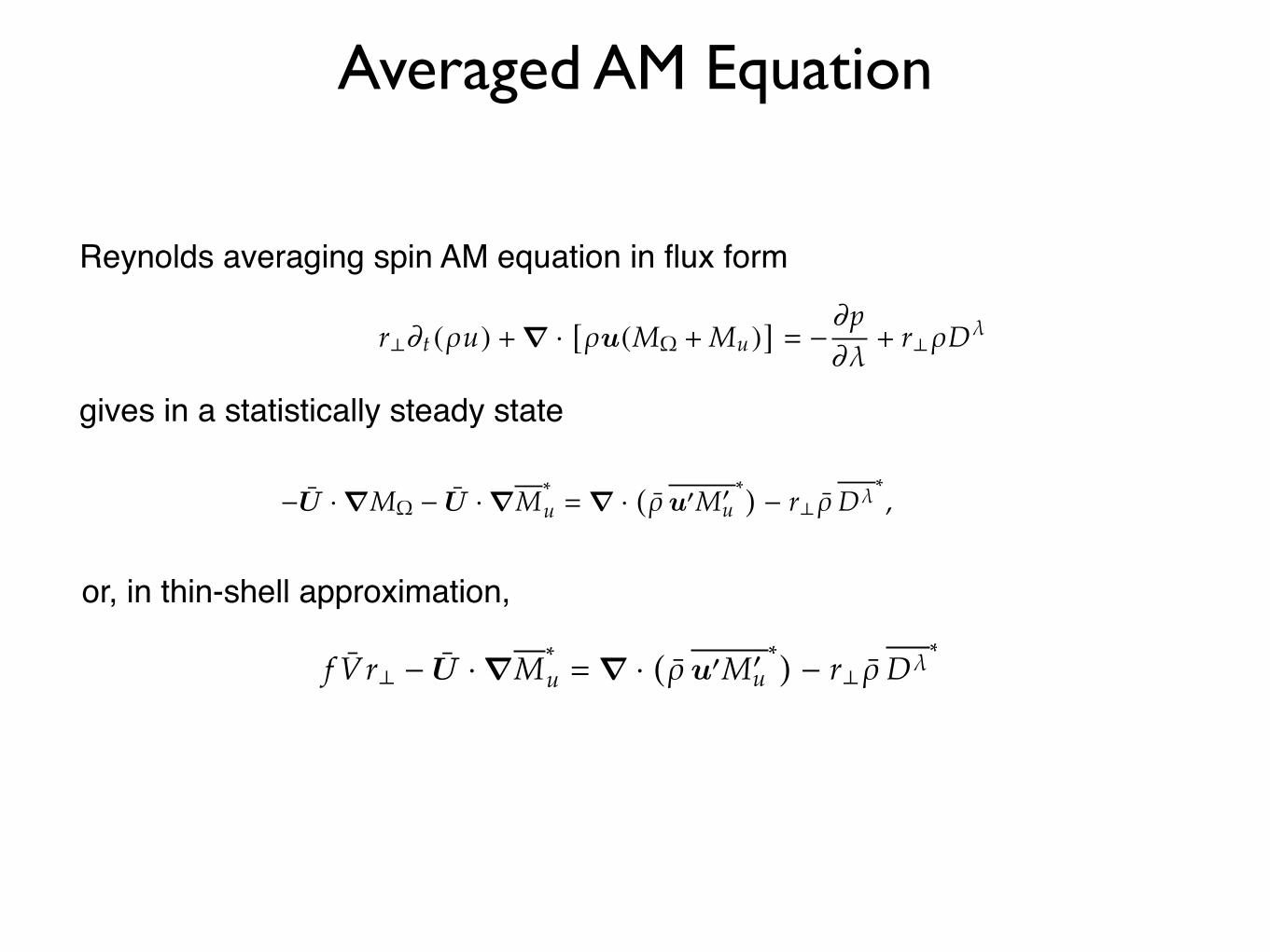
Averaged AM Equation

Reynolds averaging spin AM equation in flux form

gives in a statistically steady state



15


dMdt

1@p@

+ r?D . (1.22)




r?@t u + u ·rM + u ·rMu 1@p@

+ r?D . (1.23)



u ·rM 2r?( u) · e . (1.24)



r?@t (u) + r · u(M + Mu ) @p@

+ r?D , (1.25)




20


CHAPTER 2

Reynolds Averaging

• Eddy uxes of angular momentum in upper branches of circulations, whichextend to tropopause.

2.3 MEAN ANGULAR MOMENTUM BALANCE

density-weighted mean

(·) (·)

(2.1)

mean mass uxesU (U , V , W ) u u

In statistically steady state

U ·rM U ·rMu r · u0M0

u r?D

, (2.2a)

or, in thin-atmosphere approximation,

f V r? U ·rMu r · u0M0

u r?D

, (2.2b)

2.3.1 Free Atmosphere

low Rossby numberU ·rM r · u0M0

u

(2.3a)


f V r? r · u0M0u

(2.3b)

Coriolis torque on mean meridional ow balances eddy angular momentumux divergence where drag is weak.

2.3.2 Near Surface

low Rossby numberU ·rM r?D

, (2.4a)


f V D, (2.4b)

or, in thin-shell approximation,

20


CHAPTER 2

Reynolds Averaging




(·) (·)

(2.1)




u r?D

, (2.2a)



u r?D

, (2.2b)



u

(2.3a)


f V r? r · u0M0u

(2.3b)


2.3.2 Near Surface


, (2.4a)


f V D, (2.4b)

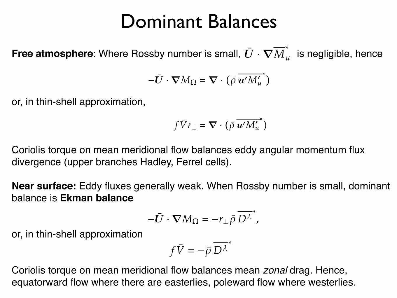
Dominant BalancesFree atmosphere: Where Rossby number is small, is negligible, hence

or, in thin-shell approximation,

Coriolis torque on mean meridional flow balances eddy angular momentum flux divergence (upper branches Hadley, Ferrel cells).

Near surface: Eddy fluxes generally weak. When Rossby number is small, dominant balance is Ekman balance

or, in thin-shell approximation

Coriolis torque on mean meridional flow balances mean zonal drag. Hence, equatorward flow where there are easterlies, poleward flow where westerlies.

20


CHAPTER 2

Reynolds Averaging




(·) (·)

(2.1)




u r?D

, (2.2a)



u r?D

, (2.2b)



u

(2.3a)


f V r? r · u0M0u

(2.3b)


2.3.2 Near Surface


, (2.4a)


f V D, (2.4b)

20


CHAPTER 2

Reynolds Averaging




(·) (·)

(2.1)




u r?D

, (2.2a)



u r?D

, (2.2b)



u

(2.3a)


f V r? r · u0M0u

(2.3b)


2.3.2 Near Surface


, (2.4a)


f V D, (2.4b)

20


CHAPTER 2

Reynolds Averaging




(·) (·)

(2.1)




u r?D

, (2.2a)



u r?D

, (2.2b)



u

(2.3a)


f V r? r · u0M0u

(2.3b)


2.3.2 Near Surface


, (2.4a)


f V D, (2.4b)

20


CHAPTER 2

Reynolds Averaging




(·) (·)

(2.1)




u r?D

, (2.2a)



u r?D

, (2.2b)



u

(2.3a)


f V r? r · u0M0u

(2.3b)


2.3.2 Near Surface


, (2.4a)


f V D, (2.4b)

20


CHAPTER 2

Reynolds Averaging




(·) (·)

(2.1)




u r?D

, (2.2a)



u r?D

, (2.2b)



u

(2.3a)


f V r? r · u0M0u

(2.3b)


2.3.2 Near Surface


, (2.4a)


f V D, (2.4b)

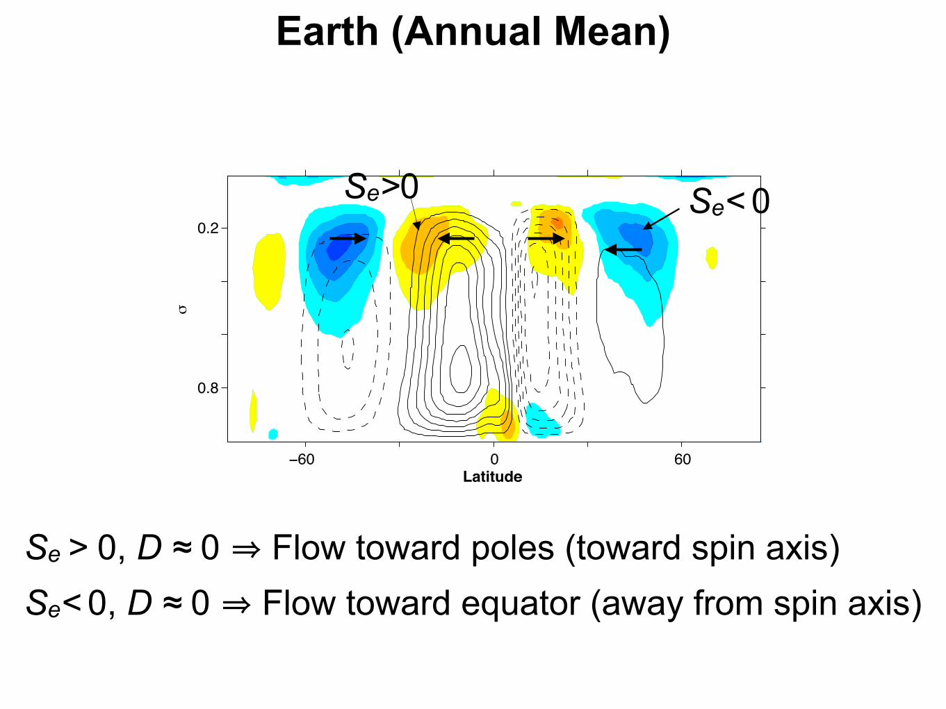
Earth (Annual Mean)

Latitude

σ

−60 0 60

0.2

0.8

Se > 0, D ≈ 0 ⇒ Flow toward poles (toward spin axis) Se< 0, D ≈ 0 ⇒ Flow toward equator (away from spin axis)

Se< 0Se>0

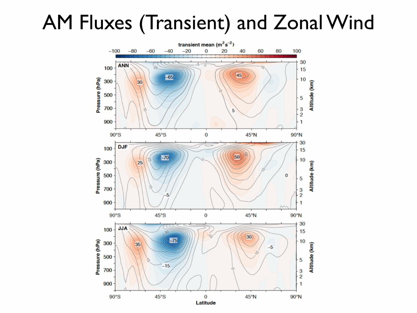
AM Fluxes (Transient) and Zonal Wind

Seasonal Cycle

(Schneider et al. 2010)climate changes only via changes in the eddy momentumflux divergence S, and possibly via changes in the width ofthe Hadley cells that can affect the relevant value of theCoriolis parameter f near their center. In this limit, changesin thermal driving affect the Hadley circulation strength onlyinsofar as they affect the eddy momentum flux divergence Sor the relevant value of the Coriolis parameter f. The localRossby number Ro above the center of a Hadley cell is anondimensional measure of how close the upper branch is tothe angular momentum–conserving limit. In the limit Ro→ 1,nonlinear momentum advection by the mean meridionalcirculation, f Ro v = v (a cos !)−1∂! (u cos !), where u is themean zonal velocity, dominates over eddy momentum fluxdivergence. In the limit Ro → 0, eddy momentum fluxdivergence dominates over nonlinear momentum advectionby the mean meridional circulation.[28] For intermediate local Rossby numbers 0 < Ro < 1,

the Hadley circulation strength can respond to climatechanges both via changes in the eddy momentum fluxdivergence and via changes in the local Rossby number. Thezonal momentum balance (10) implies that a small fractionalchange dv/v in the strength of the upper tropospheric meanmeridional mass flux must be met by changes in the eddymomentum flux divergence, dS, in the local Rossby num-ber, dRo, and in the relevant value of the Coriolis parameter,df, satisfying

"vv! "S

S þ "Ro1# Ro

# "ff: ð11Þ

For example, if Ro = 0.2 and if we neglect changes in therelevant value of the Coriolis parameter near the center of

the Hadley cells, a 10% increase in the strength of the meanmeridional mass flux requires a 10% increase in S, anincrease in Ro of dRo = 0.08 or 40%, or a combination ofthese two kinds of changes. A 40% increase in Ro impliesthe same increase in the relative vorticity (meridional shearof the zonal wind) and hence a similarly strong increase inupper tropospheric zonal winds. Such a strong increase inzonal winds would almost certainly affect the eddymomentum flux divergence S substantially. For example,according to the scaling laws described by Schneider andWalker [2008], the eddy momentum flux divergencescales at least with the square root of meridional surfacetemperature gradients and thus upper tropospheric zonalwinds (by thermal wind balance). So for small Ro in general,changes in S are strongly implicated in any changes inHadley circulation strength. Conversely, if Ro = 0.8 underthe same assumptions, a 10% increase in the strength of themean meridional mass flux requires an increase in Ro ofonly dRo = 0.02 or 2.5%, implying much subtler changes inupper tropospheric zonal winds with a weaker effect oneddy momentum fluxes. So for large Ro in general, changesin S play a reduced role in changes in Hadley circulationstrength, which therefore can respond more directly toclimate changes via changes in energetic and hydrologicbalances.[29] Earth’s Hadley cells most of the year exhibit rela-

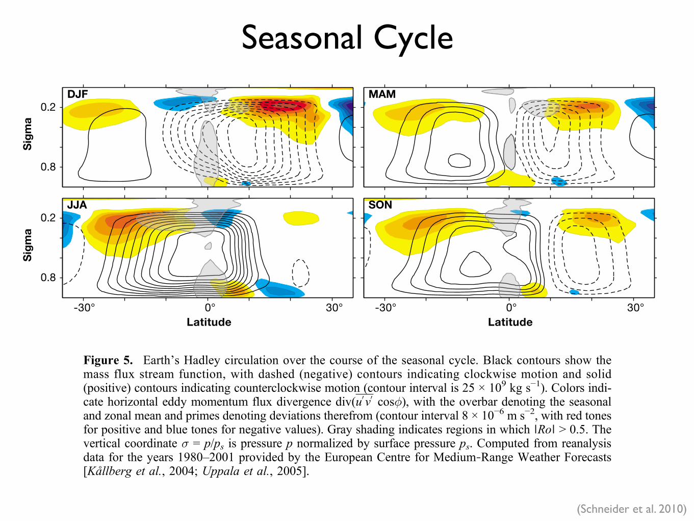
tively small local Rossby numbers in their upper branches,but local Rossby numbers and the degree to which theHadley cells are influenced by eddy momentum fluxes varyover the course of the seasonal cycle. Figure 5 showsEarth’s Hadley circulation and the horizontal eddy momen-tum flux divergence for December‐January‐February (DJF),

Figure 5. Earth’s Hadley circulation over the course of the seasonal cycle. Black contours show themass flux stream function, with dashed (negative) contours indicating clockwise motion and solid(positive) contours indicating counterclockwise motion (contour interval is 25 × 109 kg s−1). Colors indi-cate horizontal eddy momentum flux divergence div(u0v0 cos!), with the overbar denoting the seasonaland zonal mean and primes denoting deviations therefrom (contour interval 8 × 10−6 m s−2, with red tonesfor positive and blue tones for negative values). Gray shading indicates regions in which ∣Ro∣ > 0.5. Thevertical coordinate s = p/ps is pressure p normalized by surface pressure ps. Computed from reanalysisdata for the years 1980–2001 provided by the European Centre for Medium‐Range Weather Forecasts[Kållberg et al., 2004; Uppala et al., 2005].

Schneider et al.: WATER VAPOR AND CLIMATE CHANGE RG3001RG3001

9 of 22

climate changes only via changes in the eddy momentumflux divergence S, and possibly via changes in the width ofthe Hadley cells that can affect the relevant value of theCoriolis parameter f near their center. In this limit, changesin thermal driving affect the Hadley circulation strength onlyinsofar as they affect the eddy momentum flux divergence Sor the relevant value of the Coriolis parameter f. The localRossby number Ro above the center of a Hadley cell is anondimensional measure of how close the upper branch is tothe angular momentum–conserving limit. In the limit Ro→ 1,nonlinear momentum advection by the mean meridionalcirculation, f Ro v = v (a cos !)−1∂! (u cos !), where u is themean zonal velocity, dominates over eddy momentum fluxdivergence. In the limit Ro → 0, eddy momentum fluxdivergence dominates over nonlinear momentum advectionby the mean meridional circulation.[28] For intermediate local Rossby numbers 0 < Ro < 1,

the Hadley circulation strength can respond to climatechanges both via changes in the eddy momentum fluxdivergence and via changes in the local Rossby number. Thezonal momentum balance (10) implies that a small fractionalchange dv/v in the strength of the upper tropospheric meanmeridional mass flux must be met by changes in the eddymomentum flux divergence, dS, in the local Rossby num-ber, dRo, and in the relevant value of the Coriolis parameter,df, satisfying

"vv! "S

S þ "Ro1# Ro

# "ff: ð11Þ

For example, if Ro = 0.2 and if we neglect changes in therelevant value of the Coriolis parameter near the center of

the Hadley cells, a 10% increase in the strength of the meanmeridional mass flux requires a 10% increase in S, anincrease in Ro of dRo = 0.08 or 40%, or a combination ofthese two kinds of changes. A 40% increase in Ro impliesthe same increase in the relative vorticity (meridional shearof the zonal wind) and hence a similarly strong increase inupper tropospheric zonal winds. Such a strong increase inzonal winds would almost certainly affect the eddymomentum flux divergence S substantially. For example,according to the scaling laws described by Schneider andWalker [2008], the eddy momentum flux divergencescales at least with the square root of meridional surfacetemperature gradients and thus upper tropospheric zonalwinds (by thermal wind balance). So for small Ro in general,changes in S are strongly implicated in any changes inHadley circulation strength. Conversely, if Ro = 0.8 underthe same assumptions, a 10% increase in the strength of themean meridional mass flux requires an increase in Ro ofonly dRo = 0.02 or 2.5%, implying much subtler changes inupper tropospheric zonal winds with a weaker effect oneddy momentum fluxes. So for large Ro in general, changesin S play a reduced role in changes in Hadley circulationstrength, which therefore can respond more directly toclimate changes via changes in energetic and hydrologicbalances.[29] Earth’s Hadley cells most of the year exhibit rela-

tively small local Rossby numbers in their upper branches,but local Rossby numbers and the degree to which theHadley cells are influenced by eddy momentum fluxes varyover the course of the seasonal cycle. Figure 5 showsEarth’s Hadley circulation and the horizontal eddy momen-tum flux divergence for December‐January‐February (DJF),

Figure 5. Earth’s Hadley circulation over the course of the seasonal cycle. Black contours show themass flux stream function, with dashed (negative) contours indicating clockwise motion and solid(positive) contours indicating counterclockwise motion (contour interval is 25 × 109 kg s−1). Colors indi-cate horizontal eddy momentum flux divergence div(u0v0 cos!), with the overbar denoting the seasonaland zonal mean and primes denoting deviations therefrom (contour interval 8 × 10−6 m s−2, with red tonesfor positive and blue tones for negative values). Gray shading indicates regions in which ∣Ro∣ > 0.5. Thevertical coordinate s = p/ps is pressure p normalized by surface pressure ps. Computed from reanalysisdata for the years 1980–2001 provided by the European Centre for Medium‐Range Weather Forecasts[Kållberg et al., 2004; Uppala et al., 2005].

Schneider et al.: WATER VAPOR AND CLIMATE CHANGE RG3001RG3001

9 of 22

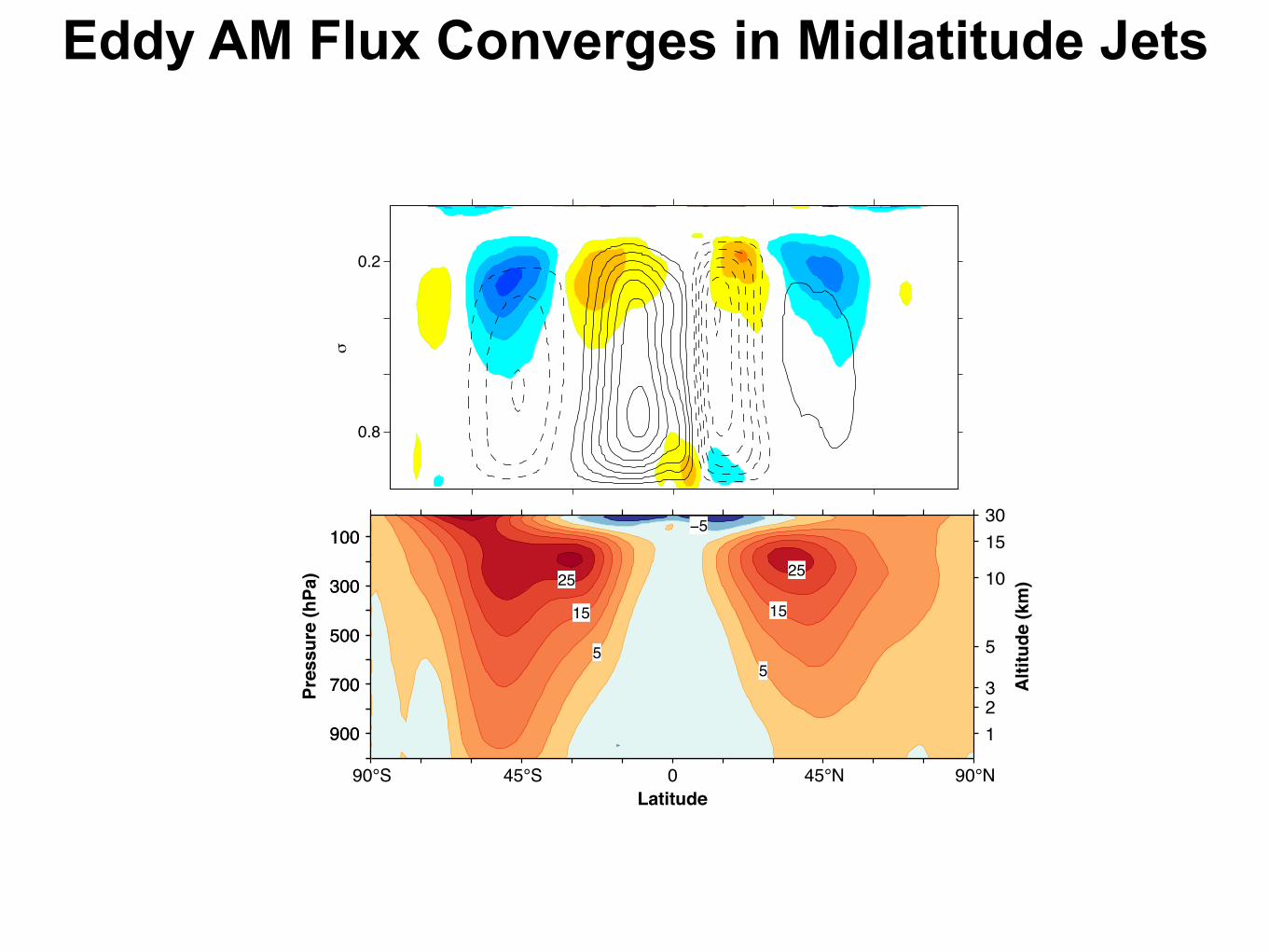
Eddy AM Flux Converges in Midlatitude Jets

Latitude

σ

−60 0 60

0.2

0.8

Latitude

Pres

sure

(hPa

) 25

15

5

25

15

5

−5

90°S 45°S 0 45°N 90°N

100

300

500

700

900

Zonal wind (m s−1)−15 −5 5 15 25 35

25

15

5

25

15

5

−5

100

300

500

700

900

Alti

tude

(km

)

123

5

10

1530

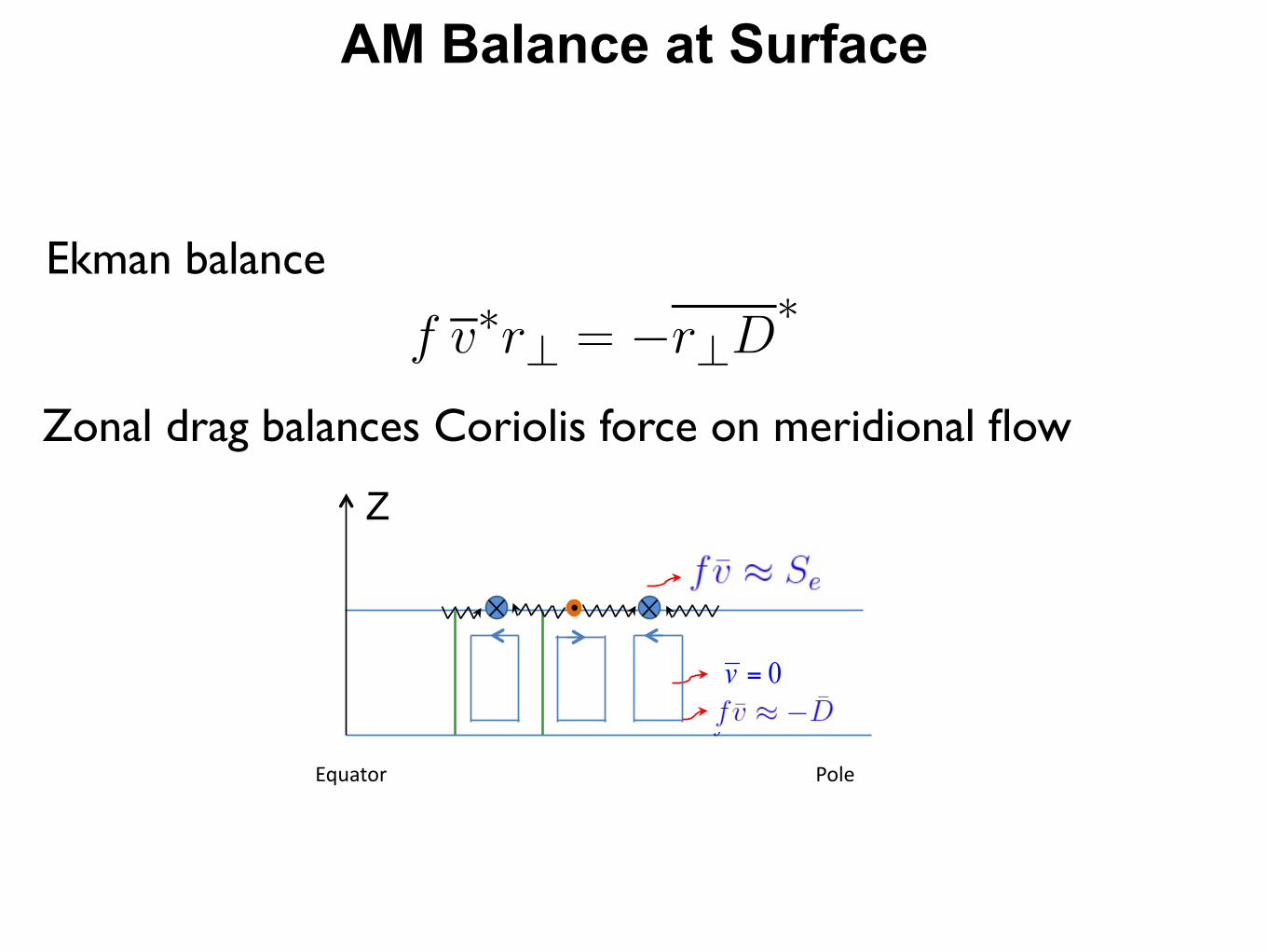
AM Balance at Surface

F = ma

a = F/m

DM

Dt= r?F

@tM + u ·rM = 1 @p + r?D

M = M

+Mu

= r2? + ur?r? = r cos

@tM +rh ·vM

+ @z

wM

= r?D

v·rhM

= rh·v0M 0

u+r?D

+O(Ro)

r? = a cos, a = const

f vr? = rh ·u0v0

r? r?D

f vr? = r?D

u ·rpM

= r?fv, f = 2 sin

Ekman balance

Zonal drag balances Coriolis force on meridional flowAngular momentum in thin atmospheres

Z

!"#$%&'( )&*+(

Away from equator, : :

In free atmosphere, eddy AM flux convergence balances Coriolis torque on mean meridional flow:

Where eddy AM flux convergence vanishes, no meridional flow (across AM contours):

Circulation must close where there is drag (or opposite AM flux convergence):

Thursday, January 7, 2010

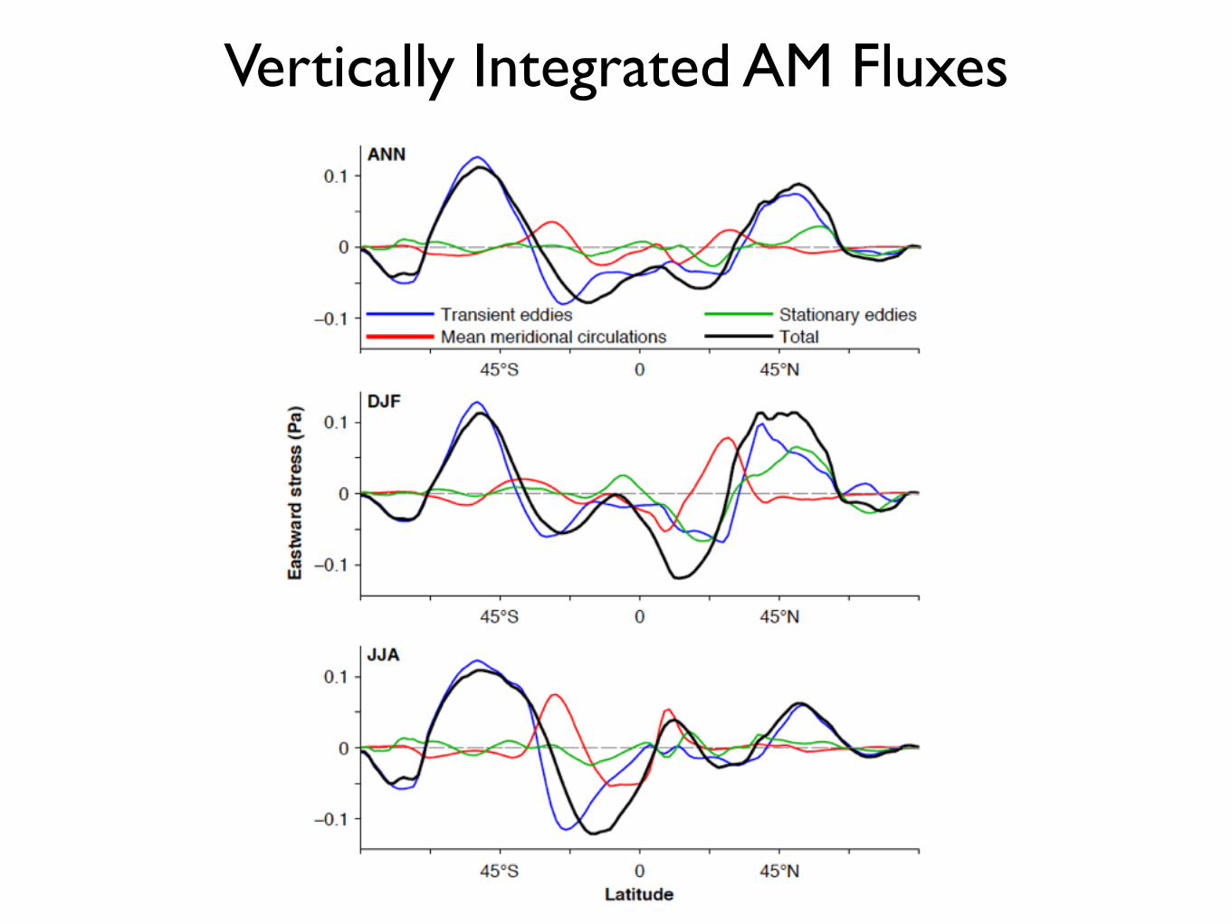
Vertically Integrated AM Fluxes

Angular Momentum - Climate Dynamics...

Documents

Transcript of Angular Momentum - Climate Dynamics...