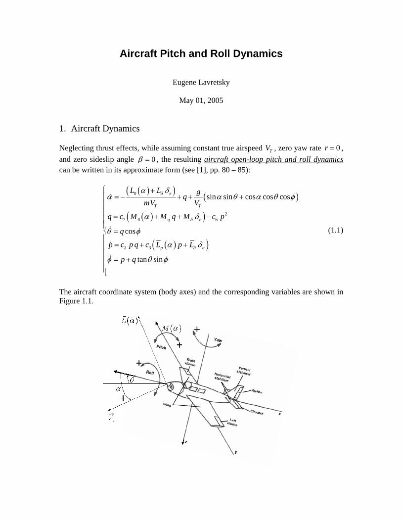
Aircraft Pitch and Roll Dynamics

Eugene Lavretsky

May 01, 2005

1. Aircraft Dynamics Neglecting thrust effects, while assuming constant true airspeed , zero yaw rate TV 0r = , and zero sideslip angle 0β = , the resulting aircraft open-loop pitch and roll dynamics can be written in its approximate form (see [1], pp. 80 – 85):

( )( ) ( )

( )( )

( )( )

0

27 0 6

2 3

sin sin cos cos cos

cos

tan sin

e

T T

q e

p a

L L gqmV V

q c M M q M c p

q

p c p q c L p L

p q

δ

δ

δ

α δα α θ α θ φ

α δ

θ φ

α δ

φ θ φ

⎧ += − + + +⎪

⎪⎪ = + + −⎪⎪

=⎨⎪

= + +⎪⎪

= +⎪⎪⎩

(1.1)

The aircraft coordinate system (body axes) and the corresponding variables are shown in Figure 1.1.

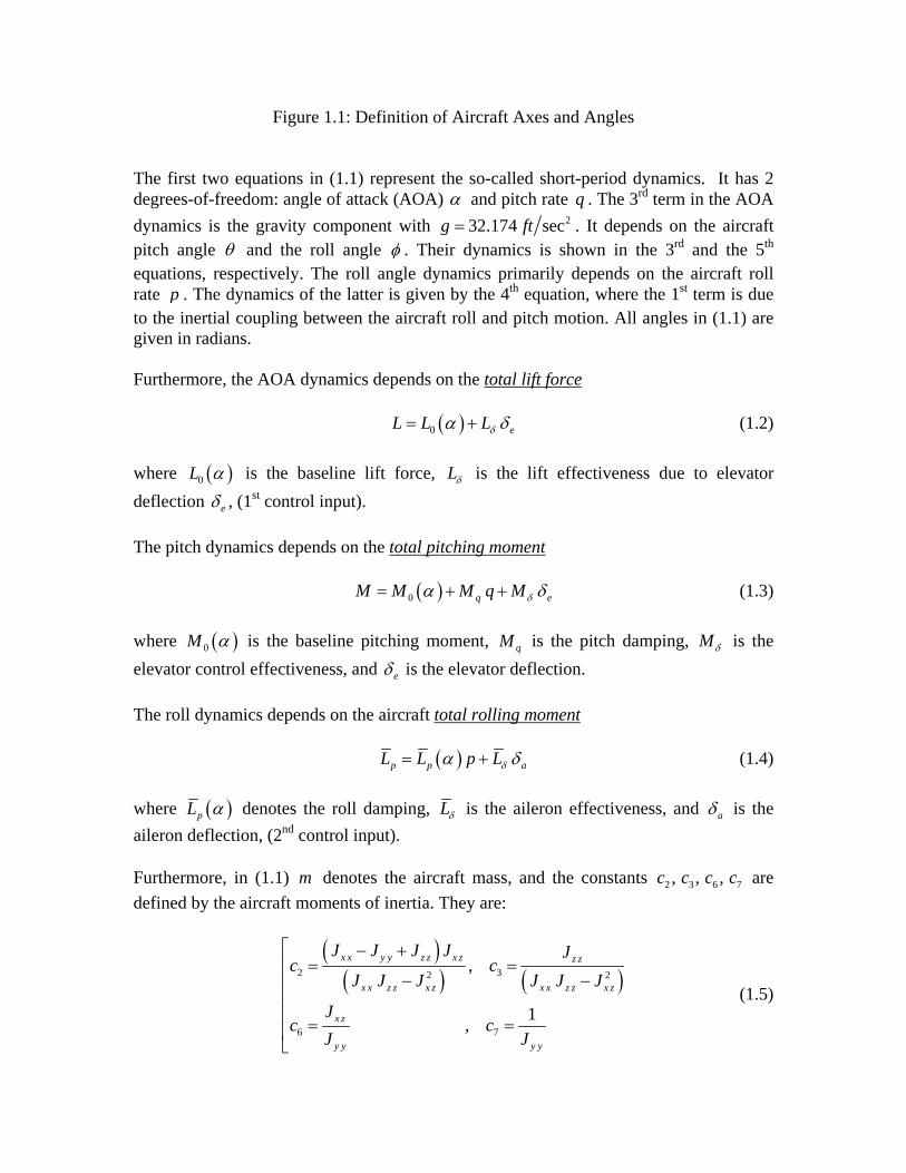
Figure 1.1: Definition of Aircraft Axes and Angles The first two equations in (1.1) represent the so-called short-period dynamics. It has 2 degrees-of-freedom: angle of attack (AOA) α and pitch rate . The 3q rd term in the AOA dynamics is the gravity component with 232.174 secg ft= . It depends on the aircraft pitch angle θ and the roll angle φ . Their dynamics is shown in the 3rd and the 5th equations, respectively. The roll angle dynamics primarily depends on the aircraft roll rate p . The dynamics of the latter is given by the 4th equation, where the 1st term is due to the inertial coupling between the aircraft roll and pitch motion. All angles in (1.1) are given in radians. Furthermore, the AOA dynamics depends on the total lift force ( )0 eL L Lδα δ= + (1.2) where ( )0L α is the baseline lift force, Lδ is the lift effectiveness due to elevator deflection eδ , (1st control input). The pitch dynamics depends on the total pitching moment ( )0 qM M M q Mδ eα δ= + + (1.3) where ( )0M α is the baseline pitching moment, qM is the pitch damping, Mδ is the elevator control effectiveness, and eδ is the elevator deflection. The roll dynamics depends on the aircraft total rolling moment ( )p pL L p Lδ aα δ= + (1.4) where ( )pL α denotes the roll damping, Lδ is the aileron effectiveness, and aδ is the aileron deflection, (2nd control input). Furthermore, in (1.1) denotes the aircraft mass, and the constants are defined by the aircraft moments of inertia. They are:

m 2 3 6 7, , ,c c c c

( )( ) ( )2 32 2

6 7

,

1,

x x y y z z x z z z

x x z z x z x x z z x z

x z

y y y y

J J J J Jc c

J J J J J J

Jc c

J J

⎡ − +⎢ = =

− −⎢⎢⎢ = =⎢⎣

(1.5)

From the state space point of view, the aircraft model (1.1) represents a 5 – dimensional nonlinear dynamical system, whose state vector ( T

px q p )α θ φ= (1.6) is assumed to be available / measurable on-line. In addition, the system is driven by the 2 – dimensional control input ( T

e a )δ δ δ= (1.7) Aircraft vertical load factor (incremental, positive up, g-s) and the roll angle zn∆ φ are the two output signals to be controlled. ( T

zy n )φ= (1.8) Neglecting thrust effects, the equation used for can be written as [2]: zn

( )sin coscos cosz

D Ln

g mα α

θ φ+

= − (1.9)

where is the aircraft D total drag force. Note that in a steady-state wings-level flight and assuming small angles, ( ) ( ) ( ) )0t t tα θ φ≈ ≈ ≈( , aircraft total lift force equals to the gross weight m g , and consequently the vertical load factor becomes approximately zero.

L

1 0zLn

g m≈ − =

Remark 1.1 The system (1.1) defines the aircraft motion starting at an equilibrium. In that sense, the dynamics is incremental relative to a trimmed AOA value ( )0α and a trimmed elevator

deflection . The model initial conditions needs to be chosen such that ( )0eδ ( ) ( )0 0α θ=

and starting with the trimmed elevator deflection ( )0eδ . The rest of the states can be initialized arbitrarily. Remark 1.2 Suppose that the roll damping pL is constant. Also suppose that the roll angle φ is zero. Then the aircraft dynamics reduces to a nonlinear model for longitudinal-only motion.

( )( ) ( )

( )( )

0

7 0

cose

T T

q e

L L gqmV V

q c M M q M

q

δ

δ

α δα θ α

α δ

θ

⎧ += − + + −⎪

⎪⎪ = + +⎨⎪

=⎪⎪⎩

(1.10)

Note that in (1.10), the quantity γ θ α= − is called the flight path angle. This is the angle between the aircraft true velocity vector TV and the horizon. Remark 1.3 Suppose that the roll damping pL does not depend strongly on α . Assume that initially,

the weight of the aircraft is balanced by its lift force, that is: ( )( )0L α = m g , and the

trimmed pitching moment is zero, that is: ( )( )0 0M α 0= . In addition, suppose that the

angles ( , , )α θ φ and the angular rates ( ),p q are sufficiently small. Introduce the lift force and the pitching moment slopes:

( )( )

( )( )0 0

,L M

L Mα αα α α α

α αα α

= =

∂ ∂= =

∂ ∂ (1.11)

Then the nonlinear aircraft model (1.1) decouples into two well-known linear pitch and roll dynamics.

( )

( )

( )

( ) ( )

7

3

Linear Pitch Dynamics :

Linear Roll Dynamics :

e

T

q e

p a

L Lq

mV

q c M M q M

q

p c L p L

p

α δ

α δ

δ

α δα

α δ

θ

δ

φ

+⎧= − +⎪

⎪⎪ = + +⎨⎪

=⎪⎪⎩

⎧ = +⎪⎨

=⎪⎩

(1.12)

Note that the two models are valid only near a trimmed flight condition, for small angles, and for small angular rates. Often the two models in (1.12) are used to perform pitch and roll control designs, independently of each other.

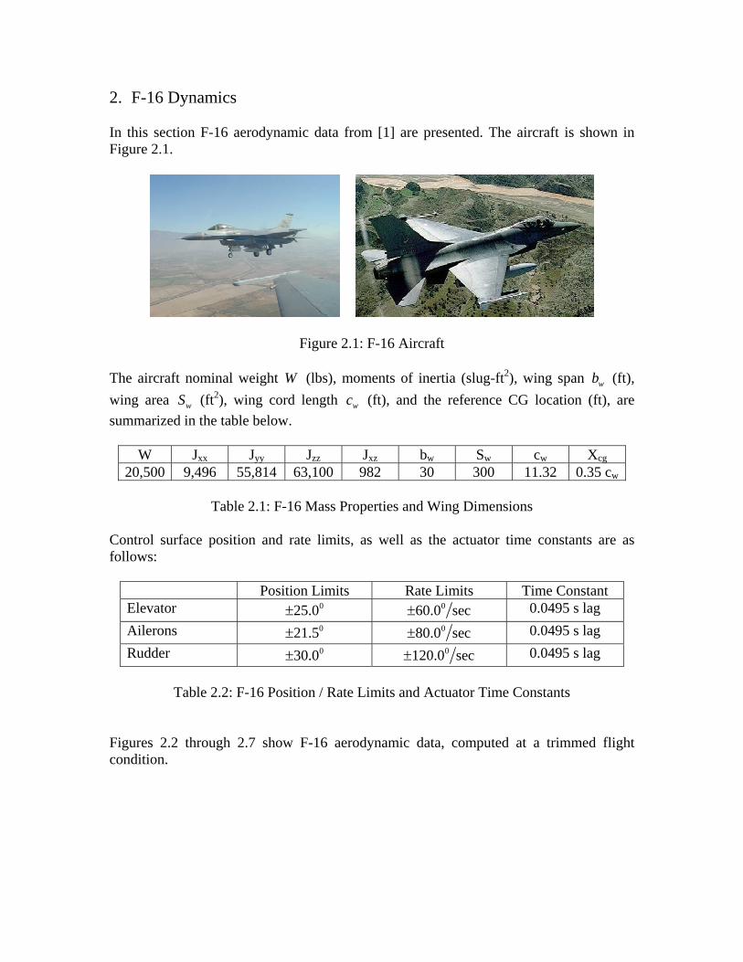
2. F-16 Dynamics In this section F-16 aerodynamic data from [1] are presented. The aircraft is shown in Figure 2.1.

Figure 2.1: F-16 Aircraft The aircraft nominal weight W (lbs), moments of inertia (slug-ft2), wing span (ft), wing area (ft

wb

wS 2), wing cord length (ft), and the reference CG location (ft), are summarized in the table below.

wc

W Jxx Jyy Jzz Jxz bw Sw cw Xcg

20,500 9,496 55,814 63,100 982 30 300 11.32 0.35 cw

Table 2.1: F-16 Mass Properties and Wing Dimensions Control surface position and rate limits, as well as the actuator time constants are as follows:

Position Limits Rate Limits Time Constant Elevator 025.0± 060.0 sec± 0.0495 s lag Ailerons 021.5± 080.0 sec± 0.0495 s lag Rudder 030.0± 0120.0 sec± 0.0495 s lag

Table 2.2: F-16 Position / Rate Limits and Actuator Time Constants

Figures 2.2 through 2.7 show F-16 aerodynamic data, computed at a trimmed flight condition.

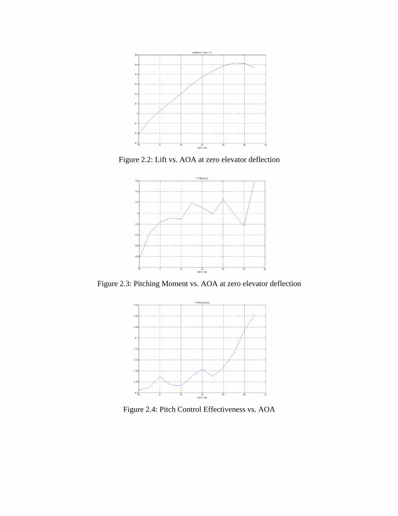
Figure 2.2: Lift vs. AOA at zero elevator deflection

Figure 2.3: Pitching Moment vs. AOA at zero elevator deflection

Figure 2.4: Pitch Control Effectiveness vs. AOA

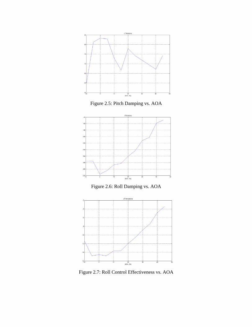
Figure 2.5: Pitch Damping vs. AOA

Figure 2.6: Roll Damping vs. AOA

Figure 2.7: Roll Control Effectiveness vs. AOA

3. Control Tracking Design Tasks The aircraft control task can be formulated as follows: Find elevator and aileron deflections (1.7) such that the vertical load factor (1.9) and the roll angle

znφ track their desired bounded commands, while the rest of the signals in

the system remain bounded. More specifically, using the F-16 data from Section 2, the following control subtasks need to be executed: a) Design a baseline controller for the system described by (1.1) to track constant and zn

φ commands, using aircraft nominal parameter values. The baseline controller can be designed using classical, linear, gain scheduled, or any other nonlinear design approach. Simulate the closed-loop tracking performance for various commanded sequences of steps in both the commanded load factor and the commanded roll angle

cmdzn

cmdφ . b) Introduce uncertainties into the aircraft aerodynamic parameters such that the baseline

closed-loop performance degrades significantly. c) Design a direct adaptive model reference control augmentation to the baseline

controller. Demonstrate benefits of the adaptive augmentation, (using simulation), such as tracking performance recovery in the presence of the system uncertainties, measurement noise, and unknown unstructured bounded disturbances.

d) Add 2nd order elevator / aileron actuator dynamics. Test and simulate closed-loop

system tracking performance. e) Simulate closed-loop system performance in the presence of control time-delays. References: [1] Stevens, B.L., Lewis F.L., Aircraft Control and Simulation, John Wiley &Sons, Inc., 1992. [2] Brumbaugh, R.W., Aircraft Model for the AIAA Controls Design Challenge, Journal of Guidance, Control, and Dynamics, Vol. 17., No. 4, July – August, 1994.