THE CFD SIMULATION OF THE FLOW AROUND THE … CFD SIMULATION OF THE FLOW AROUND THE AIRCRAFT USING...

5th

ANSA & μETA International Conference

THE CFD SIMULATION OF THE FLOW AROUND THE AIRCRAFT USING OPENFOAM AND ANSA Adam Kosík Evektor s.r.o., Czech Republic KEYWORDS – CFD simulation, mesh generation, OpenFOAM, ANSA ABSTRACT – In this paper we describe the complete process of modeling and simulation of computational fluid dynamics (CFD) problems that occur in engineering practice. We focus mainly on the simulation of the airflow around the aircraft. The fluid flow simulations are obtained with the open source CFD software package OpenFOAM. We use the solver based on the Semi-Implicit Method for Pressure-Linked Equations (SIMPLE). The important part is the preparation of the model with the software ANSA. We will describe the preprocessing including the creation and modification of the surface mesh in ANSA and the three-dimensional volume grid generation. We discuss the generation of the three-dimensional grid by the snappyHexMesh tool, which is included in the OpenFOAM package. Furthermore, we present a way of analyzing the results and some of the interesting outputs of the simulations and following analysis. The CFD simulations were performed on the computational model of the twin turboprop aircraft EV-55 Outback. We made comparison between computations made by OpenFOAM, ANSYS Fluent and measurements in a wind tunnel. The computations were performed for different model settings and computational grids. It means, that we considered laminar and turbulent flow and several combinations of the angle of attack and inlet velocity. TECHNICAL PAPER - 1. INTRODUCTION

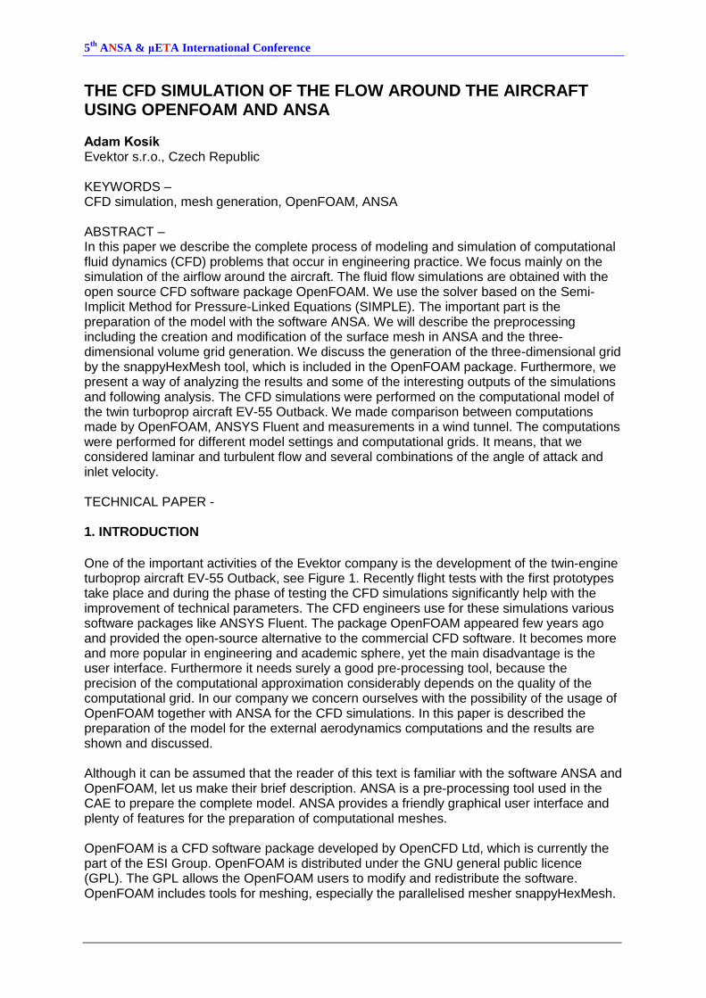
One of the important activities of the Evektor company is the development of the twin-engine turboprop aircraft EV-55 Outback, see Figure 1. Recently flight tests with the first prototypes take place and during the phase of testing the CFD simulations significantly help with the improvement of technical parameters. The CFD engineers use for these simulations various software packages like ANSYS Fluent. The package OpenFOAM appeared few years ago and provided the open-source alternative to the commercial CFD software. It becomes more and more popular in engineering and academic sphere, yet the main disadvantage is the user interface. Furthermore it needs surely a good pre-processing tool, because the precision of the computational approximation considerably depends on the quality of the computational grid. In our company we concern ourselves with the possibility of the usage of OpenFOAM together with ANSA for the CFD simulations. In this paper is described the preparation of the model for the external aerodynamics computations and the results are shown and discussed. Although it can be assumed that the reader of this text is familiar with the software ANSA and OpenFOAM, let us make their brief description. ANSA is a pre-processing tool used in the CAE to prepare the complete model. ANSA provides a friendly graphical user interface and plenty of features for the preparation of computational meshes. OpenFOAM is a CFD software package developed by OpenCFD Ltd, which is currently the part of the ESI Group. OpenFOAM is distributed under the GNU general public licence (GPL). The GPL allows the OpenFOAM users to modify and redistribute the software. OpenFOAM includes tools for meshing, especially the parallelised mesher snappyHexMesh.

5th


The mesher snappyHexMesh is used for complex geometries, it meshes to surfaces from CAD.

Figure 1 – The twin turboprop aircraft EV-55 Outback. From theoretical point of view the fluid dynamics is described by the equations for pressure, density, components of velocity and thermodynamical quantities based on conservation laws. The solver included in software like OpenFOAM is nothing more than a solver of these equations. In our computations we consider the steady-state problem. The solver contained in OpenFOAM for this problem uses the SIMPLE algorithm (Semi-Implicit Method for Pressure-Linked Equations). In order to get realistic solutions, we have to consider the turbulence. Therefore it is required to choose the suitable turbulence model. The whole computational process contains several steps. Taking into account the problem of external aerodynamics we start with the definition of the geometry of the domain occupied by the fluid flow. The domain has to be fulfilled with a suitable computational grid containing hexahedras or tetrahedras in general. Further the boundary conditions should be set, the solver options chosen and physical properties given. The results of the computation are then analyzed. We are interested about the drag and lift coefficients, the velocity streamlines and the pressure distribution. This was just a brief description of the problem and the computational process. In following paragraphs we expand the introduced subjects. 2. THEORY OF CFD AND PROBLEM DESCRIPTION The physical problem of fluid flow is described by the Navier-Stokes equations. These general equations can be simplified by specific assumptions. In our case we consider a steady-state incompressible flow. The system for steady-state incompressible flow contains a continuity equation for incompressible flow and a steady flow momentum equation. We search the velocity field and the kinematic pressure, i. e. pressure divided by the density. The density is constant by the assumption of incompressibility. Under the condition of low Mach number, i.e. the flow velocity divided by the speed of sound in fluid, even compressible fluids can be modeled as an incompressible flow. We take into account the turbulence. For the

5th


simulation of turbulent flows the formulation of the Navier-Stokes equations is modified. The OpenFOAM solver uses one of the known approaches, the time-averaged equations the Reynolds-averaged Navier-Stokes equations (RANS), supplemented with turbulence models. We solve a problem of external aerodynamics. Our task is to determine the aerodynamic characteristics of the model of the aircraft EV-55 Outback. We can compare them with the gained results from measurements on a scale model in a wind tunnel, measurements during the flight tests and the simulation results obtained using ANSYS Fluent. A general task contains information about the geometry of the aircraft, angle of attack, velocity, density and viscosity of air. The aim is to determine drag and lift coefficients of the aircraft and to create some graphical output of the pressure and velocity distribution. We use the simpleFoam solver, which is a steady-state solver for incompressible, turbulent flow. This solver uses the SIMPLE algorithm. The iterative process of this algorithm consists of several steps, that are iteratively repeated till the convergence. The steps performed by this algorithm in every iteration are following. First the boundary conditions are set. Then is obtained an approximation of the velocity field by solving the momentum equation. The mass fluxes at the cells faces are computed. The pressure equation is formulated and solved in order to obtain the pressure distribution and the underrelaxation is applied. The mass fluxes at the cell faces are corrected and so are corrected the velocities on the basis of the actual approximation of the pressure. The boundary conditions are updated and finally the convergence condition is checked. 3. PRE-PROCESSING

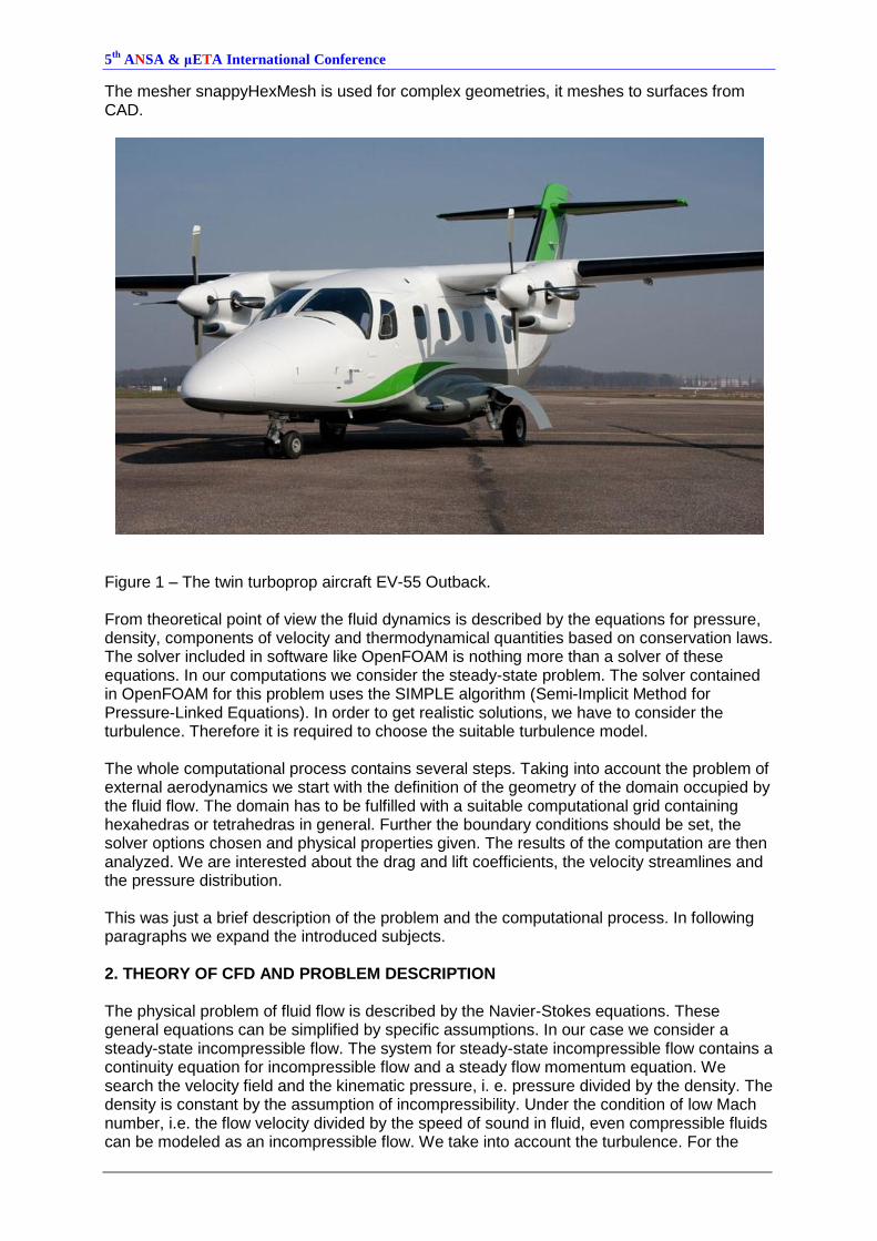
Figure 2 – The surface mesh of the whole aircraft. Mesh generation Each preparation of a CFD simulation starts with the generation of computational mesh. In the case of external aerodynamics we start from the geometry of a body and the definition of the surrounding area. The first task is to obtain a high quality surface mesh of the body. It needs to be as smooth as possible without any humps. We use ANSA for the creation and modification of the surface mesh. The surface mesh is made up of triangles. Ideally, they should all be nearly equilateral triangles. The distance between two vertices should not be too small in the scale of the whole model. This is applied to both vertices of a single triangle

5th


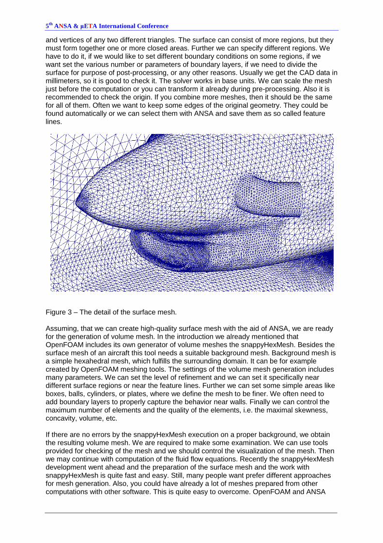
and vertices of any two different triangles. The surface can consist of more regions, but they must form together one or more closed areas. Further we can specify different regions. We have to do it, if we would like to set different boundary conditions on some regions, if we want set the various number or parameters of boundary layers, if we need to divide the surface for purpose of post-processing, or any other reasons. Usually we get the CAD data in millimeters, so it is good to check it. The solver works in base units. We can scale the mesh just before the computation or you can transform it already during pre-processing. Also it is recommended to check the origin. If you combine more meshes, then it should be the same for all of them. Often we want to keep some edges of the original geometry. They could be found automatically or we can select them with ANSA and save them as so called feature lines.

Figure 3 – The detail of the surface mesh. Assuming, that we can create high-quality surface mesh with the aid of ANSA, we are ready for the generation of volume mesh. In the introduction we already mentioned that OpenFOAM includes its own generator of volume meshes the snappyHexMesh. Besides the surface mesh of an aircraft this tool needs a suitable background mesh. Background mesh is a simple hexahedral mesh, which fulfills the surrounding domain. It can be for example created by OpenFOAM meshing tools. The settings of the volume mesh generation includes many parameters. We can set the level of refinement and we can set it specifically near different surface regions or near the feature lines. Further we can set some simple areas like boxes, balls, cylinders, or plates, where we define the mesh to be finer. We often need to add boundary layers to properly capture the behavior near walls. Finally we can control the maximum number of elements and the quality of the elements, i.e. the maximal skewness, concavity, volume, etc. If there are no errors by the snappyHexMesh execution on a proper background, we obtain the resulting volume mesh. We are required to make some examination. We can use tools provided for checking of the mesh and we should control the visualization of the mesh. Then we may continue with computation of the fluid flow equations. Recently the snappyHexMesh development went ahead and the preparation of the surface mesh and the work with snappyHexMesh is quite fast and easy. Still, many people want prefer different approaches for mesh generation. Also, you could have already a lot of meshes prepared from other computations with other software. This is quite easy to overcome. OpenFOAM and ANSA

5th


also offers a wide range of converters from other formats. Namely as example we can convert from the files of ANSYS, CFX4, Fluent, Gambit, GMSH, or STAR-CD. Case settings Let's describe the settings of solved cases. We consider steady-state incompressible viscous turbulent flow. For the computations we used different geometries of the turboprop aircraft EV-55 Outback, because one set of computations is with model with landing gear retracted and the other with landing gear extended. In presented computations we consider just the initial position of flaps. The meshes were generated with the aid of ANSA and the snappyHexMesh tool or with TGrid. The fluid is considered to be air. Because of the

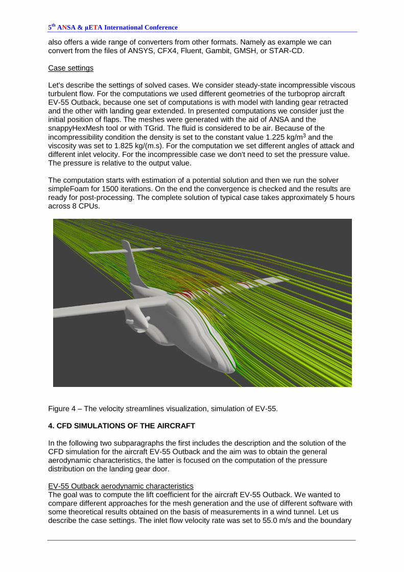
incompressibility condition the density is set to the constant value 1.225 kg/m3 and the viscosity was set to 1.825 kg/(m.s). For the computation we set different angles of attack and different inlet velocity. For the incompressible case we don't need to set the pressure value. The pressure is relative to the output value. The computation starts with estimation of a potential solution and then we run the solver simpleFoam for 1500 iterations. On the end the convergence is checked and the results are ready for post-processing. The complete solution of typical case takes approximately 5 hours across 8 CPUs.

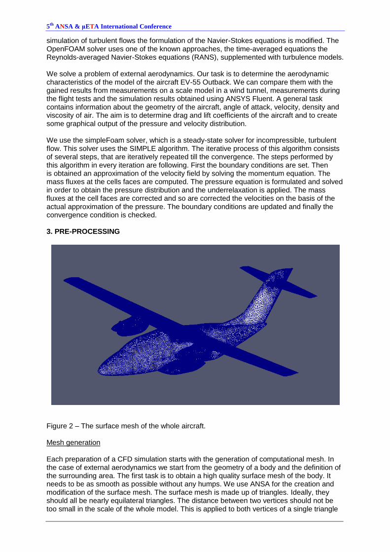
Figure 4 – The velocity streamlines visualization, simulation of EV-55. 4. CFD SIMULATIONS OF THE AIRCRAFT In the following two subparagraphs the first includes the description and the solution of the CFD simulation for the aircraft EV-55 Outback and the aim was to obtain the general aerodynamic characteristics, the latter is focused on the computation of the pressure distribution on the landing gear door. EV-55 Outback aerodynamic characteristics The goal was to compute the lift coefficient for the aircraft EV-55 Outback. We wanted to compare different approaches for the mesh generation and the use of different software with some theoretical results obtained on the basis of measurements in a wind tunnel. Let us describe the case settings. The inlet flow velocity rate was set to 55.0 m/s and the boundary

5th


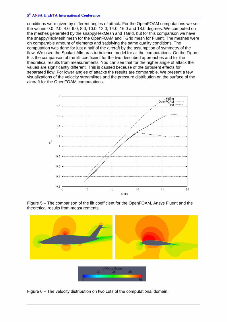
conditions were given by different angles of attack. For the OpenFOAM computations we set the values 0.0, 2.0, 4.0, 6.0, 8.0, 10.0, 12.0, 14.0, 16.0 and 18.0 degrees. We computed on the meshes generated by the snappyHexMesh and TGrid, but for this comparison we have the snappyHexMesh mesh for the OpenFOAM and TGrid mesh for Fluent. The meshes were on comparable amount of elements and satisfying the same quality conditions. The computation was done for just a half of the aircraft by the assumption of symmetry of the flow. We used the Spalart-Allmaras turbulence model for all the computations. On the Figure 5 is the comparison of the lift coefficient for the two described approaches and for the theoretical results from measurements. You can see that for the higher angle of attack the values are significantly different. This is caused because of the turbulent effects for separated flow. For lower angles of attacks the results are comparable. We present a few visualizations of the velocity streamlines and the pressure distribution on the surface of the aircraft for the OpenFOAM computations.

Figure 5 – The comparison of the lift coefficient for the OpenFOAM, Ansys Fluent and the theoretical results from measurements.

Figure 6 – The velocity distribution on two cuts of the computational domain.

5th


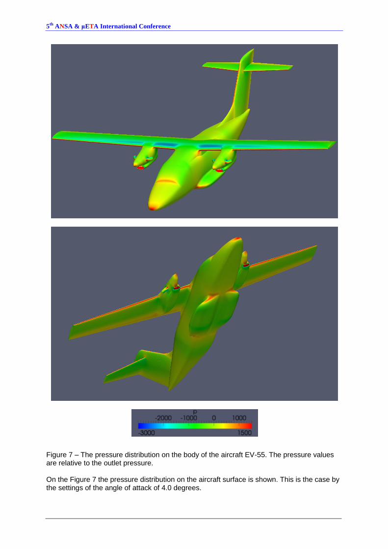
Figure 7 – The pressure distribution on the body of the aircraft EV-55. The pressure values are relative to the outlet pressure. On the Figure 7 the pressure distribution on the aircraft surface is shown. This is the case by the settings of the angle of attack of 4.0 degrees.

5th


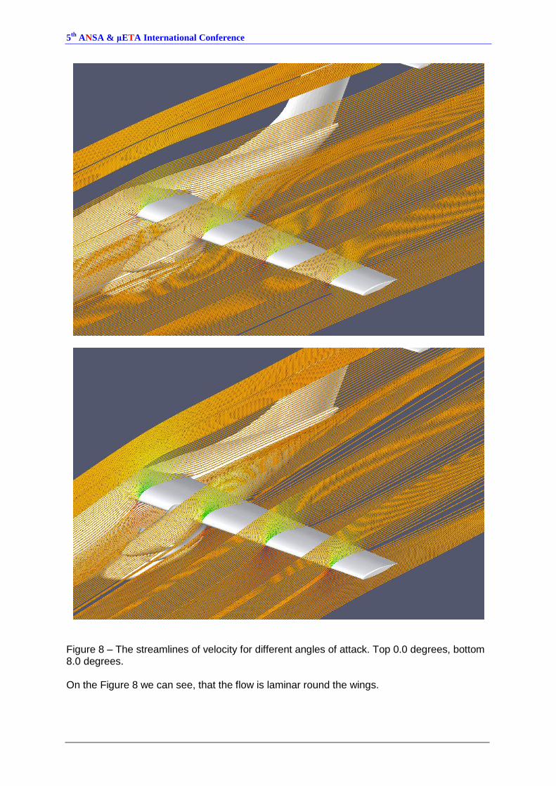
Figure 8 – The streamlines of velocity for different angles of attack. Top 0.0 degrees, bottom 8.0 degrees. On the Figure 8 we can see, that the flow is laminar round the wings.

5th


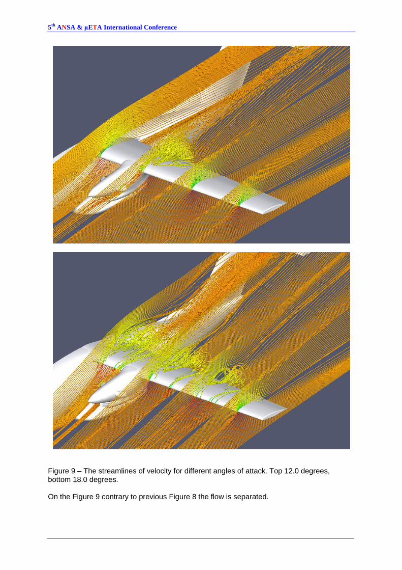
Figure 9 – The streamlines of velocity for different angles of attack. Top 12.0 degrees, bottom 18.0 degrees. On the Figure 9 contrary to previous Figure 8 the flow is separated.

5th


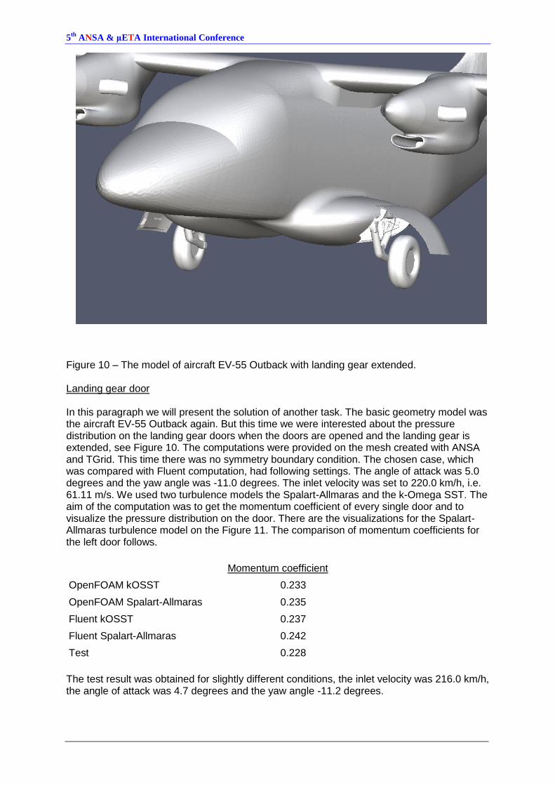
Figure 10 – The model of aircraft EV-55 Outback with landing gear extended. Landing gear door In this paragraph we will present the solution of another task. The basic geometry model was the aircraft EV-55 Outback again. But this time we were interested about the pressure distribution on the landing gear doors when the doors are opened and the landing gear is extended, see Figure 10. The computations were provided on the mesh created with ANSA and TGrid. This time there was no symmetry boundary condition. The chosen case, which was compared with Fluent computation, had following settings. The angle of attack was 5.0 degrees and the yaw angle was -11.0 degrees. The inlet velocity was set to 220.0 km/h, i.e. 61.11 m/s. We used two turbulence models the Spalart-Allmaras and the k-Omega SST. The aim of the computation was to get the momentum coefficient of every single door and to visualize the pressure distribution on the door. There are the visualizations for the Spalart-Allmaras turbulence model on the Figure 11. The comparison of momentum coefficients for the left door follows.

Momentum coefficient

OpenFOAM kOSST 0.233

OpenFOAM Spalart-Allmaras 0.235

Fluent kOSST 0.237

Fluent Spalart-Allmaras 0.242

Test 0.228

The test result was obtained for slightly different conditions, the inlet velocity was 216.0 km/h, the angle of attack was 4.7 degrees and the yaw angle -11.2 degrees.

5th


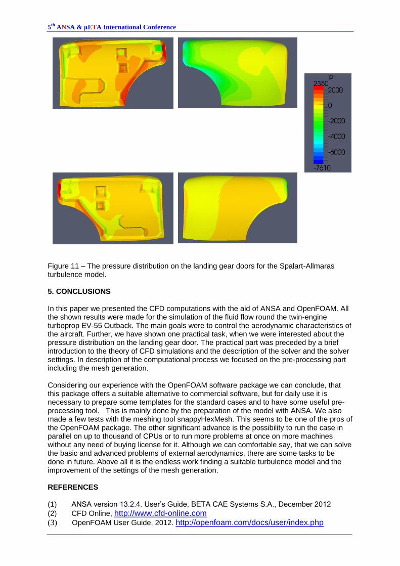
Figure 11 – The pressure distribution on the landing gear doors for the Spalart-Allmaras turbulence model. 5. CONCLUSIONS In this paper we presented the CFD computations with the aid of ANSA and OpenFOAM. All the shown results were made for the simulation of the fluid flow round the twin-engine turboprop EV-55 Outback. The main goals were to control the aerodynamic characteristics of the aircraft. Further, we have shown one practical task, when we were interested about the pressure distribution on the landing gear door. The practical part was preceded by a brief introduction to the theory of CFD simulations and the description of the solver and the solver settings. In description of the computational process we focused on the pre-processing part including the mesh generation. Considering our experience with the OpenFOAM software package we can conclude, that this package offers a suitable alternative to commercial software, but for daily use it is necessary to prepare some templates for the standard cases and to have some useful pre-processing tool. This is mainly done by the preparation of the model with ANSA. We also made a few tests with the meshing tool snappyHexMesh. This seems to be one of the pros of the OpenFOAM package. The other significant advance is the possibility to run the case in parallel on up to thousand of CPUs or to run more problems at once on more machines without any need of buying license for it. Although we can comfortable say, that we can solve the basic and advanced problems of external aerodynamics, there are some tasks to be done in future. Above all it is the endless work finding a suitable turbulence model and the improvement of the settings of the mesh generation. REFERENCES (1) ANSA version 13.2.4. User’s Guide, BETA CAE Systems S.A., December 2012

(2) CFD Online, http://www.cfd-online.com

(3) OpenFOAM User Guide, 2012. http://openfoam.com/docs/user/index.php

http://www.cfd-online.com/

http://openfoam.com/docs/user/index.php

THE CFD SIMULATION OF THE FLOW AROUND THE … CFD SIMULATION OF THE FLOW AROUND THE AIRCRAFT USING...

Documents

Transcript of THE CFD SIMULATION OF THE FLOW AROUND THE … CFD SIMULATION OF THE FLOW AROUND THE AIRCRAFT USING...