Kernels and Support Vector Machines
28
Seminar 2 Kernels and Support Vector Machines Edgar Marca Supervisor: DSc. André M.S. Barreto Petrópolis, Rio de Janeiro - Brazil September 2nd, 2015 1 / 28
-
Upload
edgar-marca -
Category
Science
-
view
416 -
download
0
Transcript of Kernels and Support Vector Machines
Seminar 2Kernels
andSupport Vector Machines
Edgar Marca
Supervisor: DSc. André M.S. Barreto
Petrópolis, Rio de Janeiro - BrazilSeptember 2nd, 2015
1 / 28
Kernels
Kernels
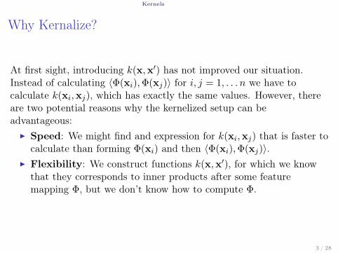
Why Kernalize?
At first sight, introducing k(x,x′) has not improved our situation.Instead of calculating ⟨Φ(xi),Φ(xj)⟩ for i, j = 1, . . . n we have tocalculate k(xi,xj), which has exactly the same values. However, thereare two potential reasons why the kernelized setup can beadvantageous:
▶ Speed: We might find and expression for k(xi,xj) that is faster tocalculate than forming Φ(xi) and then ⟨Φ(xi),Φ(xj)⟩.
▶ Flexibility: We construct functions k(x,x′), for which we knowthat they corresponds to inner products after some featuremapping Φ, but we don’t know how to compute Φ.
3 / 28
Kernels
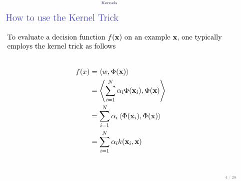
How to use the Kernel Trick
To evaluate a decision function f(x) on an example x, one typicallyemploys the kernel trick as follows
f(x) = ⟨w,Φ(x)⟩
=
⟨N∑i=1
αiΦ(xi),Φ(x)
⟩
=
N∑i=1
αi ⟨Φ(xi),Φ(x)⟩
=
N∑i=1
αik(xi,x)
4 / 28
How to proof that a functionis a kernel?
Kernels
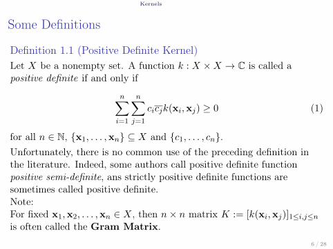
Some Definitions
Definition 1.1 (Positive Definite Kernel)Let X be a nonempty set. A function k : X ×X → C is called apositive definite if and only if
n∑i=1
n∑j=1
cicjk(xi,xj) ≥ 0 (1)
for all n ∈ N, {x1, . . . ,xn} ⊆ X and {c1, . . . , cn}.Unfortunately, there is no common use of the preceding definition inthe literature. Indeed, some authors call positive definite functionpositive semi-definite, ans strictly positive definite functions aresometimes called positive definite.Note:For fixed x1,x2, . . . ,xn ∈ X, then n× n matrix K := [k(xi,xj)]1≤i,j≤n
is often called the Gram Matrix.
6 / 28
Kernels
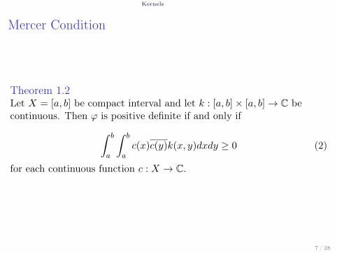
Mercer Condition
Theorem 1.2Let X = [a, b] be compact interval and let k : [a, b]× [a, b] → C becontinuous. Then φ is positive definite if and only if∫ b
a
∫ b
ac(x)c(y)k(x, y)dxdy ≥ 0 (2)
for each continuous function c : X → C.
7 / 28
Kernels
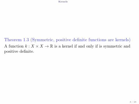
Theorem 1.3 (Symmetric, positive definite functions are kernels)A function k : X ×X → R is a kernel if and only if is symmetric andpositive definite.
8 / 28

Kernels
Theorem 1.4Let k1, k2 . . . are arbitrary positive definite kernels in X ×X, where Xis not an empty set.
▶ The set of positive definite kernels is a closed convex cone, that is,1. If α1, α2 ≥ 0, then α1k1 + α2k2 is positive definitive.2. If k(x,x′) := lim
n→∞kn(x,x
′) exists for all x,x′ then k is positivedefinitive.
▶ The product k1.k2 is positive definite kernel.▶ Assume that for i = 1, 2 ki is a positive definite kernel on Xi ×Xi,
where Xi is a nonempty set. Then the tensor product k1 ⊗ k2 andthe direct sum k1 ⊕ k2 are positive definite kernels on(X1 ×X2)× (X1 ×X2).
▶ Suppose that Y is not an empty set and let f : Y → X anyarbitrary function then k(x,y) = k1(f(x), f(y)) is a positivedefinite kernel over Y × Y .
9 / 28

Kernel Families
Kernels Kernel Families
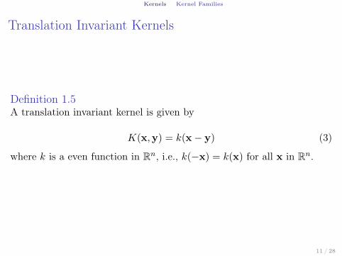
Translation Invariant Kernels
Definition 1.5A translation invariant kernel is given by
K(x,y) = k(x− y) (3)
where k is a even function in Rn, i.e., k(−x) = k(x) for all x in Rn.
11 / 28
Kernels Kernel Families
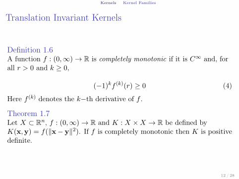
Translation Invariant Kernels
Definition 1.6A function f : (0,∞) → R is completely monotonic if it is C∞ and, forall r > 0 and k ≥ 0,
(−1)kf (k)(r) ≥ 0 (4)
Here f (k) denotes the k−th derivative of f .
Theorem 1.7Let X ⊂ Rn, f : (0,∞) → R and K : X ×X → R be defined byK(x,y) = f(∥x− y∥2). If f is completely monotonic then K is positivedefinite.
12 / 28
Kernels Kernel Families
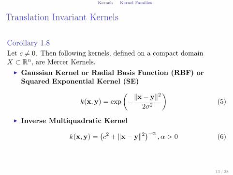
Translation Invariant Kernels
Corollary 1.8Let c ̸= 0. Then following kernels, defined on a compact domainX ⊂ Rn, are Mercer Kernels.
▶ Gaussian Kernel or Radial Basis Function (RBF) orSquared Exponential Kernel (SE)
k(x,y) = exp
(−∥x− y∥2
2σ2
)(5)
▶ Inverse Multiquadratic Kernel
k(x,y) =(c2 + ∥x− y∥2
)−α, α > 0 (6)
13 / 28
Kernels Kernel Families
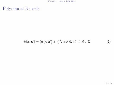
Polynomial Kernels
k(x,x′) = (α⟨x,x′⟩+ c)d, α > 0, c ≥ 0, d ∈ Z (7)
14 / 28
Kernels Kernel Families
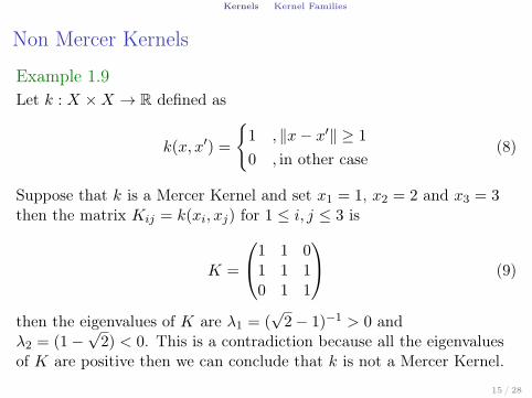
Non Mercer Kernels
Example 1.9Let k : X ×X → R defined as
k(x, x′) =
{1 , ∥x− x′∥ ≥ 1
0 , in other case(8)
Suppose that k is a Mercer Kernel and set x1 = 1, x2 = 2 and x3 = 3then the matrix Kij = k(xi, xj) for 1 ≤ i, j ≤ 3 is
K =
1 1 01 1 10 1 1
(9)
then the eigenvalues of K are λ1 = (√2− 1)−1 > 0 and
λ2 = (1−√2) < 0. This is a contradiction because all the eigenvalues
of K are positive then we can conclude that k is not a Mercer Kernel.
15 / 28
Kernels Kernel Families
References for Kernels
[3] C. Berg, J. Reus, and P. Ressel. Harmonic Analysis onSemigroups: Theory of Positive Definite and Related Functions.Springer Science+Business Media, LLV, 1984.
[9] Felipe Cucker and Ding Xuan Zhou. Learning Theory.Cambridge University Press, 2007.
[47] Ingo Steinwart and Christmannm Andreas. Support VectorMachines. 2008.
16 / 28
Support Vector Machines
Applications SVM
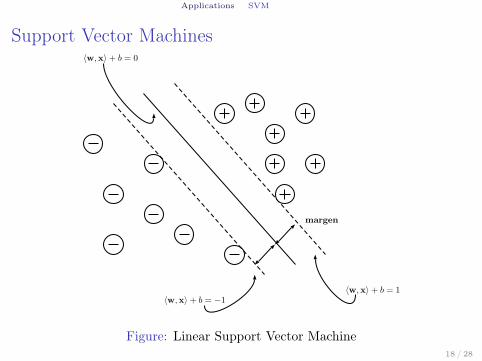
Support Vector Machines
〈w,x〉 + b = 1
〈w,x〉 + b = −1
〈w,x〉 + b = 0
margen
Figure: Linear Support Vector Machine18 / 28
Applications SVM
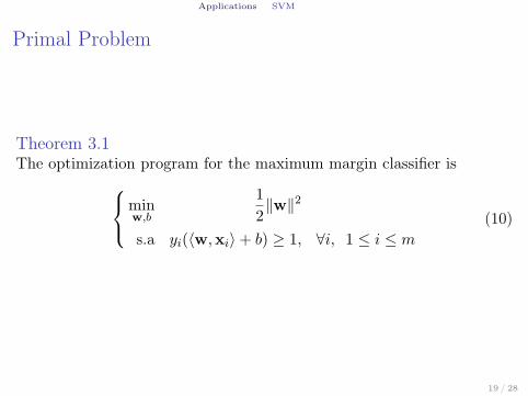
Primal Problem
Theorem 3.1The optimization program for the maximum margin classifier ismin
w,b
1
2∥w∥2
s.a yi(⟨w,xi⟩+ b) ≥ 1, ∀i, 1 ≤ i ≤ m
(10)
19 / 28
Applications SVM
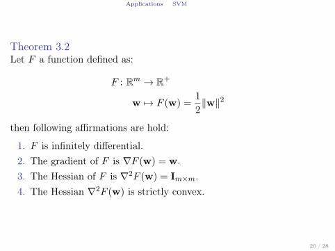
Theorem 3.2Let F a function defined as:
F : Rm → R+
w 7→ F (w) =1
2∥w∥2
then following affirmations are hold:
1. F is infinitely differential.2. The gradient of F is ∇F (w) = w.3. The Hessian of F is ∇2F (w) = Im×m.4. The Hessian ∇2F (w) is strictly convex.
20 / 28
Applications SVM
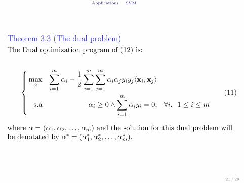
Theorem 3.3 (The dual problem)The Dual optimization program of (12) is:
maxα
m∑i=1
αi −1
2
m∑i=1
m∑j=1
αiαjyiyj⟨xi,xj⟩
s.a αi ≥ 0 ∧m∑i=1
αiyi = 0, ∀i, 1 ≤ i ≤ m
(11)
where α = (α1, α2, . . . , αm) and the solution for this dual problem willbe denotated by α∗ = (α∗
1, α∗2, . . . , α
∗m).
21 / 28
Applications SVM
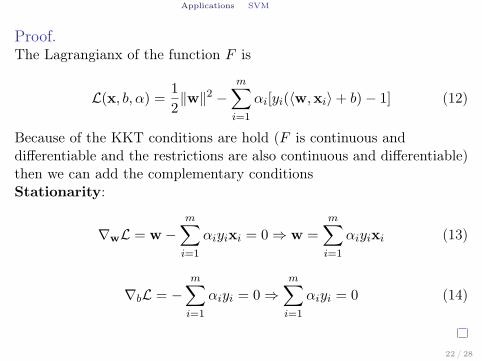
Proof.The Lagrangianx of the function F is
L(x, b, α) = 1
2∥w∥2 −
m∑i=1
αi[yi(⟨w,xi⟩+ b)− 1] (12)
Because of the KKT conditions are hold (F is continuous anddifferentiable and the restrictions are also continuous and differentiable)then we can add the complementary conditionsStationarity:
∇wL = w −m∑i=1
αiyixi = 0 ⇒ w =
m∑i=1
αiyixi (13)
∇bL = −m∑i=1
αiyi = 0 ⇒m∑i=1
αiyi = 0 (14)
22 / 28
Applications SVM
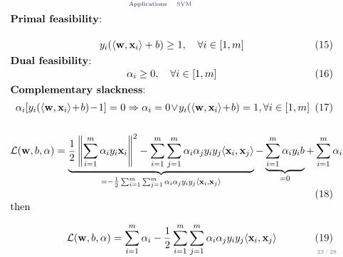
Primal feasibility:
yi(⟨w,xi⟩+ b) ≥ 1, ∀i ∈ [1,m] (15)Dual feasibility:
αi ≥ 0, ∀i ∈ [1,m] (16)Complementary slackness:
αi[yi(⟨w,xi⟩+b)−1] = 0 ⇒ αi = 0∨yi(⟨w,xi⟩+b) = 1, ∀i ∈ [1,m] (17)
L(w, b, α) =1
2
∥∥∥∥∥m∑i=1
αiyixi
∥∥∥∥∥2
−m∑i=1
m∑j=1
αiαjyiyj⟨xi,xj⟩︸ ︷︷ ︸=− 1
2
∑mi=1
∑mj=1 αiαjyiyj⟨xi,xj⟩
−m∑i=1
αiyib︸ ︷︷ ︸=0
+
m∑i=1
αi
(18)then
L(w, b, α) =
m∑i=1
αi −1
2
m∑i=1
m∑j=1
αiαjyiyj⟨xi,xj⟩ (19)23 / 28
Applications SVM
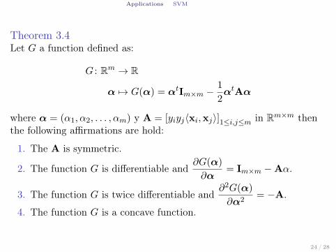
Theorem 3.4Let G a function defined as:
G : Rm → R
α 7→ G(α) = αtIm×m − 1
2αtAα
where α = (α1, α2, . . . , αm) y A = [yiyj⟨xi,xj⟩]1≤i,j≤m in Rm×m thenthe following affirmations are hold:
1. The A is symmetric.
2. The function G is differentiable and∂G(α)
∂α= Im×m −Aα.
3. The function G is twice differentiable and∂2G(α)
∂α2= −A.
4. The function G is a concave function.
24 / 28
Applications SVM
Linear Support Vector Machines
We will called Support Vector Machines to the decision function definedby
f(x) = sign (⟨w,x⟩+ b) = sign
(m∑i=1
α∗i yi⟨xi,x⟩+ b
)(20)
Where▶ m is the number of training points.▶ α∗
i are the lagrange multipliers of the dual problem (13).
25 / 28
Applications Non Linear SVM
Non Linear Support Vector Machines
We will called Non Linear Support Vector Machines to the decisionfunction defined by
f(x) = sign (⟨w,Φ(x)⟩+ b) = sign
(m∑i=1
α∗i yi⟨Φ(xi),Φ(x)⟩+ b
)(21)
Where▶ m is the number of training points.▶ α∗
i are the lagrange multipliers of the dual problem (13).
26 / 28
Applications Non Linear SVM
Applying the Kernel Trick
Using the kernel trick we can replace ⟨Φ(xi),Φ(x)⟩ by a kernel k(xi,x)
f(x) = sign
(m∑i=1
α∗i yik(xi,x) + b
)(22)
Where▶ m is the number of training points.▶ α∗
i are the lagrange multipliers of the dual problem (13).
27 / 28
Applications Non Linear SVM
References for Support Vector Machines
[31] Mehryar Mohri, Afshin Rostamizadeh, and Ameet Talwalkar.Foundations of Machine Learning. The MIT Press, 2012.
28 / 28