Support Vector Machines (Contd.), Classification Loss

Support Vector Machines (Contd.),Classification Loss Functions and Regularizers

Piyush Rai

CS5350/6350: Machine Learning

September 13, 2011

(CS5350/6350) SVMs, Loss Functions and Regularization September 13, 2011 1 / 18

SVM (Recap)

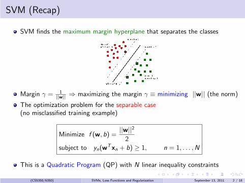
SVM finds the maximum margin hyperplane that separates the classes

Margin γ = 1||w|| ⇒ maximizing the margin γ ≡ minimizing ||w|| (the norm)

The optimization problem for the separable case(no misclassified training example)

Minimize f (w, b) =||w||2

2

subject to yn(wTxn + b) ≥ 1, n = 1, . . . ,N

This is a Quadratic Program (QP) with N linear inequality constraints


SVM: The Optimization Problem

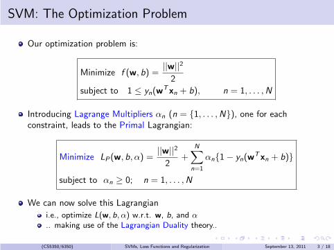
Our optimization problem is:


2

subject to 1 ≤ yn(wTxn + b), n = 1, . . . ,N

Introducing Lagrange Multipliers αn (n = {1, . . . ,N}), one for eachconstraint, leads to the Primal Lagrangian:

Minimize LP(w, b, α) =||w||2

2+

N∑

n=1

αn{1− yn(wTxn + b)}

subject to αn ≥ 0; n = 1, . . . ,N

We can now solve this Lagrangian

i.e., optimize L(w, b, α) w.r.t. w, b, and α

.. making use of the Lagrangian Duality theory..


SVM: The Optimization Problem

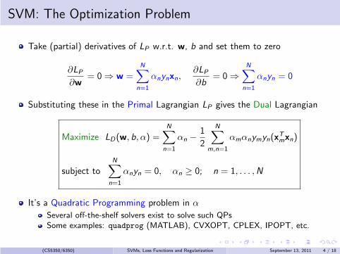
Take (partial) derivatives of LP w.r.t. w, b and set them to zero

∂LP

∂w= 0 ⇒ w =

N∑

n=1

αnynxn,∂LP

∂b= 0 ⇒

N∑

n=1

αnyn = 0

Substituting these in the Primal Lagrangian LP gives the Dual Lagrangian

Maximize LD(w, b, α) =

N∑

n=1

αn −1

2

N∑

m,n=1

αmαnymyn(xTmxn)

subject toN∑

n=1

αnyn = 0, αn ≥ 0; n = 1, . . . ,N

It’s a Quadratic Programming problem in α

Several off-the-shelf solvers exist to solve such QPsSome examples: quadprog (MATLAB), CVXOPT, CPLEX, IPOPT, etc.


SVM: The Solution

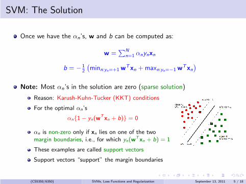
Once we have the αn’s, w and b can be computed as:

w =∑N

n=1 αnynxn

b = − 12

(

minn:yn=+1 wTxn +maxn:yn=−1 w

Txn)

Note: Most αn’s in the solution are zero (sparse solution)

Reason: Karush-Kuhn-Tucker (KKT) conditions

For the optimal αn’s

αn{1− yn(wTxn + b)} = 0

αn is non-zero only if xn lies on one of the twomargin boundaries, i.e., for which yn(w

Txn + b) = 1

These examples are called support vectors

Support vectors “support” the margin boundaries


SVM - Non-separable case

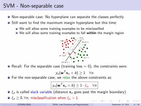
Non-separable case: No hyperplane can separate the classes perfectly

Still want to find the maximum margin hyperplane but this time:

We will allow some training examples to be misclassifiedWe will allow some training examples to fall within the margin region

Recall: For the separable case (training loss = 0), the constraints were:

yn(wTxn + b) ≥ 1 ∀n

For the non-separable case, we relax the above constraints as:

yn(wTxn + b) ≥ 1−ξn ∀n

ξn is called slack variable (distance xn goes past the margin boundary)

ξn ≥ 0, ∀n, misclassification when ξn > 1


SVM - Non-separable case

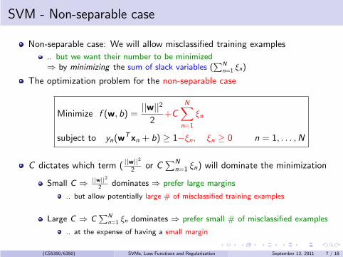
Non-separable case: We will allow misclassified training examples

.. but we want their number to be minimized⇒ by minimizing the sum of slack variables (

∑N

n=1 ξn)

The optimization problem for the non-separable case


2+C

N∑

n=1

ξn

subject to yn(wTxn + b) ≥ 1−ξn, ξn ≥ 0 n = 1, . . . ,N

C dictates which term ( ||w||2

2 or C∑N

n=1 ξn) will dominate the minimization

Small C ⇒ ||w||2

2dominates ⇒ prefer large margins

.. but allow potentially large # of misclassified training examples

Large C ⇒ C∑N

n=1 ξn dominates ⇒ prefer small # of misclassified examples

.. at the expense of having a small margin


SVM - Non-separable case: The Optimization Problem

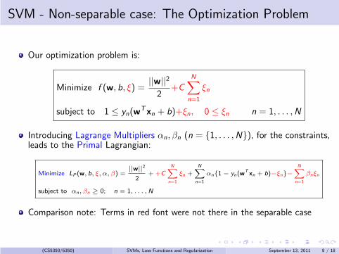
Our optimization problem is:

Minimize f (w, b, ξ) =||w||2

2+C

N∑

n=1

ξn

subject to 1 ≤ yn(wTxn + b)+ξn, 0 ≤ ξn n = 1, . . . ,N

Introducing Lagrange Multipliers αn, βn (n = {1, . . . ,N}), for the constraints,leads to the Primal Lagrangian:

Minimize LP (w, b, ξ, α, β) =||w||2

2+ +C

N∑

n=1

ξn +N∑

n=1

αn{1 − yn(wTxn + b)−ξn}−

N∑

n=1

βnξn

subject to αn, βn ≥ 0; n = 1, . . . ,N

Comparison note: Terms in red font were not there in the separable case


SVM - Non-separable case: The Optimization Problem

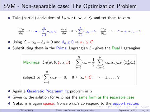
Take (partial) derivatives of LP w.r.t. w, b, ξn and set them to zero

∂LP

∂w= 0 ⇒ w =

N∑

n=1

αnynxn,∂LP

∂b= 0 ⇒

N∑

n=1

αnyn = 0,∂LP

∂ξn= 0 ⇒ C − αn − βn = 0

Using C − αn − βn = 0 and βn ≥ 0 ⇒ αn ≤ C

Substituting these in the Primal Lagrangian LP gives the Dual Lagrangian

Maximize LD(w, b, ξ, α, β) =

N∑

n=1

αn −1

2

N∑

m,n=1

αmαnymyn(xTmxn)

subject to

N∑

n=1

αnyn = 0, 0 ≤ αn≤ C ; n = 1, . . . ,N

Again a Quadratic Programming problem in α

Given α, the solution for w, b has the same form as the separable case

Note: α is again sparse. Nonzero αn’s correspond to the support vectors


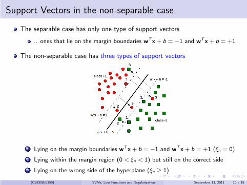
Support Vectors in the non-separable case

The separable case has only one type of support vectors

.. ones that lie on the margin boundaries wTx+ b = −1 and wTx+ b = +1

The non-separable case has three types of support vectors

1 Lying on the margin boundaries wTx+ b = −1 and wTx+ b = +1 (ξn = 0)

2 Lying within the margin region (0 < ξn < 1) but still on the correct side

3 Lying on the wrong side of the hyperplane (ξn ≥ 1)


Support Vector Machines: some notes

Training time of the standard SVM is O(N3) (have to solve the QP)

Can be prohibitive for large datasets

Lots of research has gone into speeding up the SVMs

Many approximate QP solvers are used to speed up SVMs

Online training (e.g., using stochastic gradient descent)

Several extensions exist

Nonlinear separation boundaries by applying the Kernel Trick (next class)

More than 2 classes (multiclass classification)

Structured outputs (structured prediction)

Real-valued outputs (support vector regression)

Popular SVM implementations: libSVM, SVMLight, SVM-struct, etc.

Also http://www.kernel-machines.org/software


http://www.kernel-machines.org/software

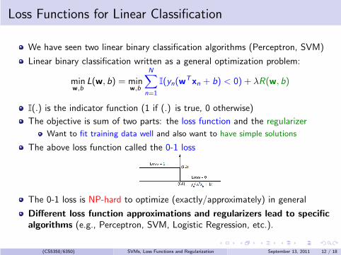
Loss Functions for Linear Classification

We have seen two linear binary classification algorithms (Perceptron, SVM)

Linear binary classification written as a general optimization problem:

minw,b

L(w, b) = minw,b

N∑

n=1

I(yn(wTxn + b) < 0) + λR(w, b)

I(.) is the indicator function (1 if (.) is true, 0 otherwise)

The objective is sum of two parts: the loss function and the regularizer

Want to fit training data well and also want to have simple solutions

The above loss function called the 0-1 loss

The 0-1 loss is NP-hard to optimize (exactly/approximately) in general

Different loss function approximations and regularizers lead to specific

algorithms (e.g., Perceptron, SVM, Logistic Regression, etc.).


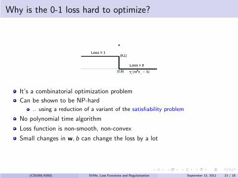
Why is the 0-1 loss hard to optimize?

It’s a combinatorial optimization problem

Can be shown to be NP-hard

.. using a reduction of a variant of the satisfiability problem

No polynomial time algorithm

Loss function is non-smooth, non-convex

Small changes in w, b can change the loss by a lot


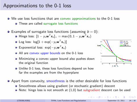
Approximations to the 0-1 loss

We use loss functions that are convex approximations to the 0-1 loss

These are called surrogate loss functions

Examples of surrogate loss functions (assuming b = 0):Hinge loss: [1− ynw

Txn]+ = max{0, 1− ynwTxn}

Log loss: log[1 + exp(−ynwTxn)]

Exponential loss: exp(−ynwTxn)

All are convex upper bounds on the 0-1 loss

Minimizing a convex upper bound also pushes downthe original function

Unlike 0-1 loss, these loss functions depend on howfar the examples are from the hyperplane

Apart from convexity, smoothness is the other desirable for loss functions

Smoothness allows using gradient (or stochastic gradient) descentNote: hinge loss is not smooth at (1,0) but subgradient descent can be used


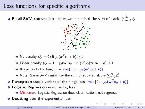
Loss functions for specific algorithms

Recall SVM non-separable case: we minimized the sum of slacks∑N

n=1 ξn

No penalty (ξn = 0) if yn(wTxn + b) ≥ 1

Linear penalty (ξn = 1− yn(wTxn + b)) if yn(w

Txn + b) < 1

It’s precisely the hinge loss max{0, 1− yn(wTxn + b)}

Note: Some SVMs minimize the sum of squared slacks∑N

n=1 ξ2n

Perceptron uses a variant of the hinge loss: max{0,−yn(wTxn + b)}

Logistic Regression uses the log loss

Misnomer: Logistic Regression does classification, not regression!

Boosting uses the exponential loss


Regularizers

Recall: The optimization problem for regularized linear binary classification:

minw,b

L(w, b) = minw,b

N∑

n=1

I(yn(wTxn + b) < 0) + λR(w, b)

We have already seen the approximation choices for the 0-1 loss function

What about the regularizer term R(w, b) to ensure simple solutions?

The regularizer R(w, b) determines what each entry wd of w looks like

Ideally, we want most entries wd of w be zero, so prediction depends only ona small number of features (for which wd 6= 0). Desired minimization:

Rcnt(w, b) =

D∑

d=1

I(wd 6= 0)

Rcnt(w, b) is NP-hard to minimize, so its approximations are used

A good approximation is to make the individual wd ’s small

Small wd ⇒ small changes in some feature xd won’t affect prediction by much

Small individual weights wd is a notion of function simplicity


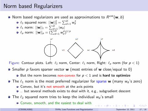
Norm based Regularizers

Norm based regularizers are used as approximations to Rcnt(w, b)

ℓ2 squared norm: ||w||22 =∑D

d=1 w2d

ℓ1 norm: ||w||1 =∑D

d=1 |wd |

ℓp norm: ||w||p = (∑D

d=1 wp

d )1/p

Figure: Contour plots. Left: ℓ2 norm, Center: ℓ1 norm, Right: ℓp norm (for p < 1)

Smaller p favors sparser vector w (most entries of w close/equal to 0)

But the norm becomes non-convex for p < 1 and is hard to optimize

The ℓ1 norm is the most preferred regularizer for sparse w (many wd ’s zero)

Convex, but it’s not smooth at the axis points.. but several methods exists to deal with it, e.g., subgradient descent

The ℓ2 squared norm tries to keep the individual wd ’s small

Convex, smooth, and the easiest to deal with


Next class..

Introduction to Kernels

Nonlinear classification algorithms

Kernelized PerceptronKernelized Support Vector Machines


Support Vector Machines (Contd.), Classification Loss

Documents

Transcript of Support Vector Machines (Contd.), Classification Loss