![Renewal theorems for random walks in random …Renewal theorems for random walks in random scenery by Erdös, Feller and Pollard [10], Blackwell [1, 2]. Extensions to multi-dimensional](https://static.fdocument.org/doc/165x107/5f3f99f70d1cf75e8f4f5f95/renewal-theorems-for-random-walks-in-random-renewal-theorems-for-random-walks-in.jpg)
Random Walks, Random Fields, and Graph Kernels...Random Walks, Random Fields, and Graph Kernels John...
28
Random Walks, Random Fields, and Graph Kernels John Lafferty School of Computer Science Carnegie Mellon University Based on work with Avrim Blum, Zoubin Ghahramani, Risi Kondor Mugizi Rwebangira, Jerry Zhu
Transcript of Random Walks, Random Fields, and Graph Kernels...Random Walks, Random Fields, and Graph Kernels John...
Random Walks, Random Fields, andGraph Kernels
John Lafferty
School of Computer Science
Carnegie Mellon University
Based on work with
Avrim Blum, Zoubin Ghahramani, Risi KondorMugizi Rwebangira, Jerry Zhu
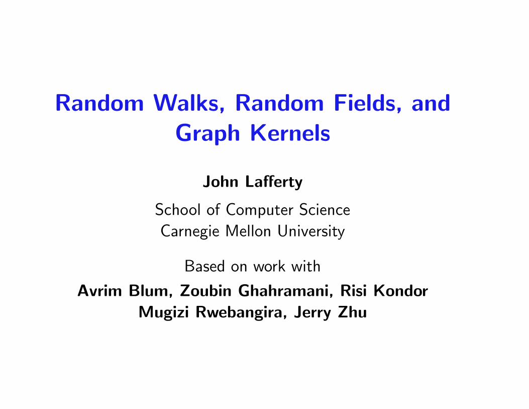
Outline
Graph Kernels −−−→ Random Fieldsx
y
Random Walks ←−−− Continuous Fields
1
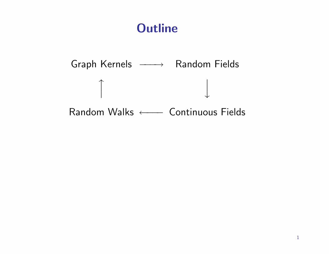
Using a Kernel
f(x) =∑N
i=1 αi yi 〈x, xi〉 f(x) =∑N
i=1 αi yi K(x, xi)
2
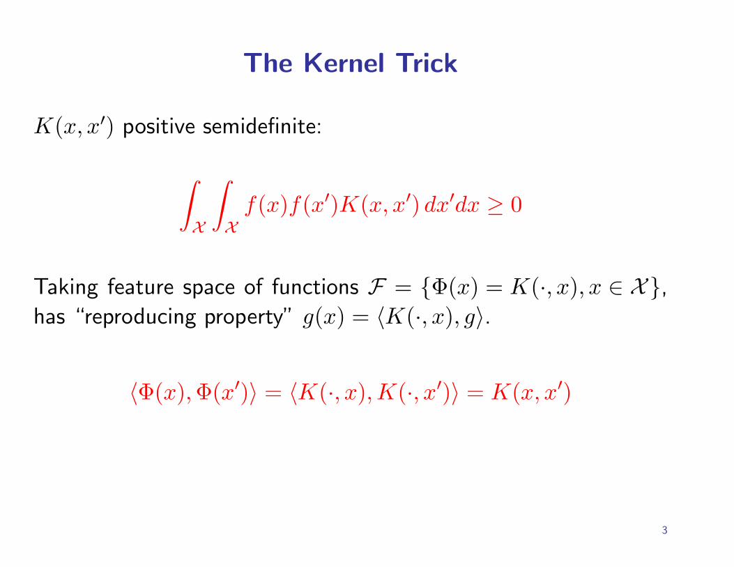
The Kernel Trick
K(x, x′) positive semidefinite:
∫
X
∫
Xf(x)f(x′)K(x, x′) dx′dx ≥ 0
Taking feature space of functions F = {Φ(x) = K(·, x), x ∈ X},has “reproducing property” g(x) = 〈K(·, x), g〉.
〈Φ(x), Φ(x′)〉 = 〈K(·, x),K(·, x′)〉 = K(x, x′)
3
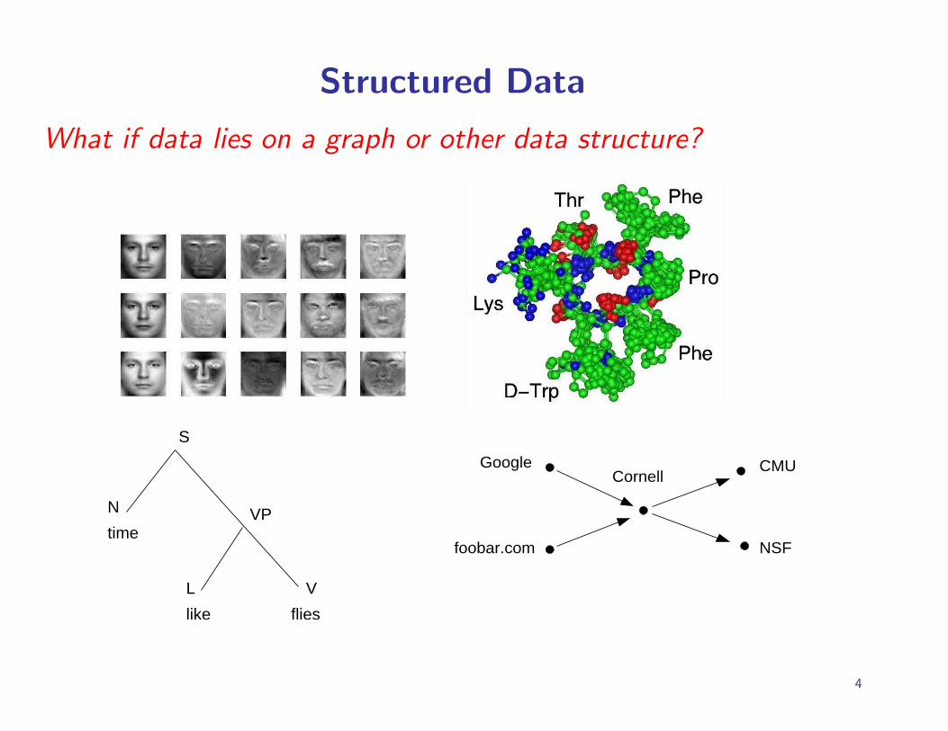
Structured Data
What if data lies on a graph or other data structure?
L V
flies
VP
S
N
time
like
CornellCMU
NSF
foobar.com
4
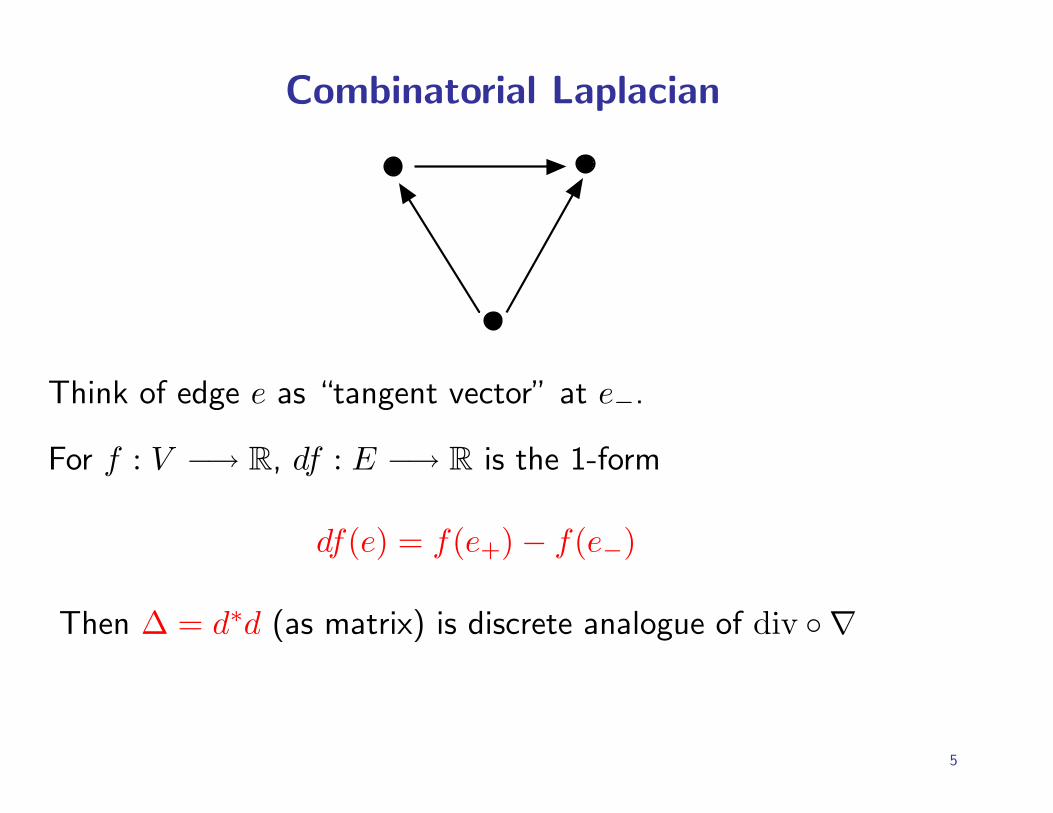
Combinatorial Laplacian
��������������� ��
����
����� ������������������������������������������������������������������������������������������������������������������������������������������������
������������������������������������������������������������������������������������������������������������������������������������������������
����������������������������������������������������������������
����������������������������������������������������������������
Think of edge e as “tangent vector” at e−.
For f : V −→ R, df : E −→ R is the 1-form
df(e) = f(e+)− f(e−)
Then ∆ = d∗d (as matrix) is discrete analogue of div ◦ ∇
5
Combinatorial Laplacian
It is an averaging operator
∆f(x) =∑y∼x
wxy(f(x)− f(y))
= d(x) f(x)−∑x∼y
wxyf(y)
We say f is harmonic if ∆f = 0.
Since 〈f, ∆g〉 = 〈df, dg〉, ∆ is self-adjoint and positive.
6
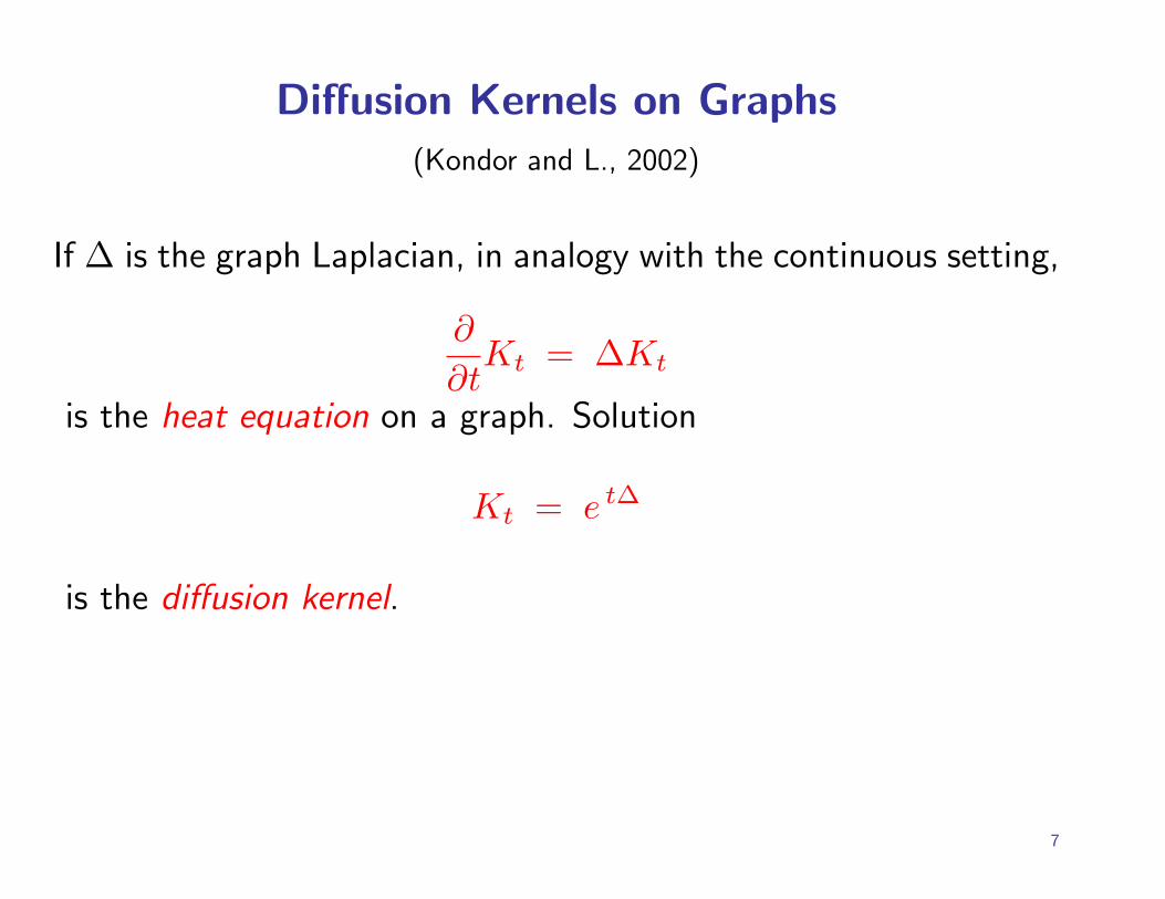
Diffusion Kernels on Graphs(Kondor and L., 2002)
If ∆ is the graph Laplacian, in analogy with the continuous setting,
∂
∂tKt = ∆Kt
is the heat equation on a graph. Solution
Kt = e t∆
is the diffusion kernel.
7
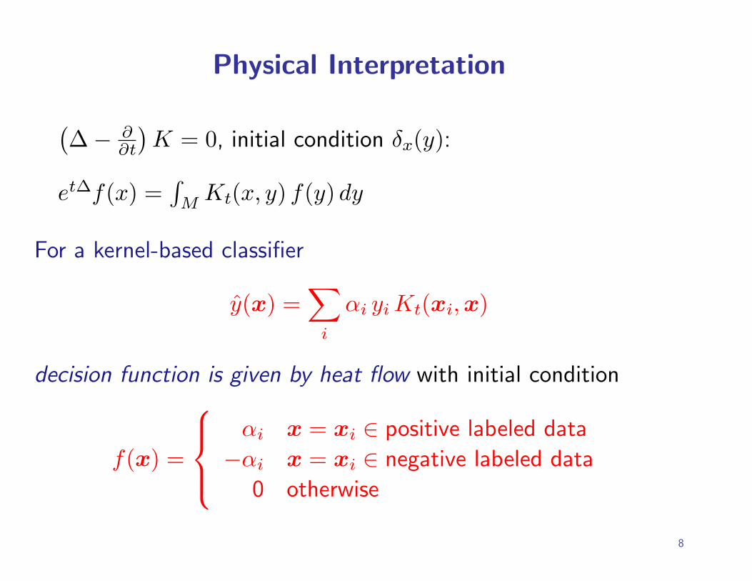
Physical Interpretation
(∆− ∂
∂t
)K = 0, initial condition δx(y):
et∆f(x) =∫
MKt(x, y) f(y) dy
For a kernel-based classifier
y(x) =∑
i
αi yi Kt(xi, x)
decision function is given by heat flow with initial condition
f(x) =
αi x = xi ∈ positive labeled data
−αi x = xi ∈ negative labeled data
0 otherwise
8
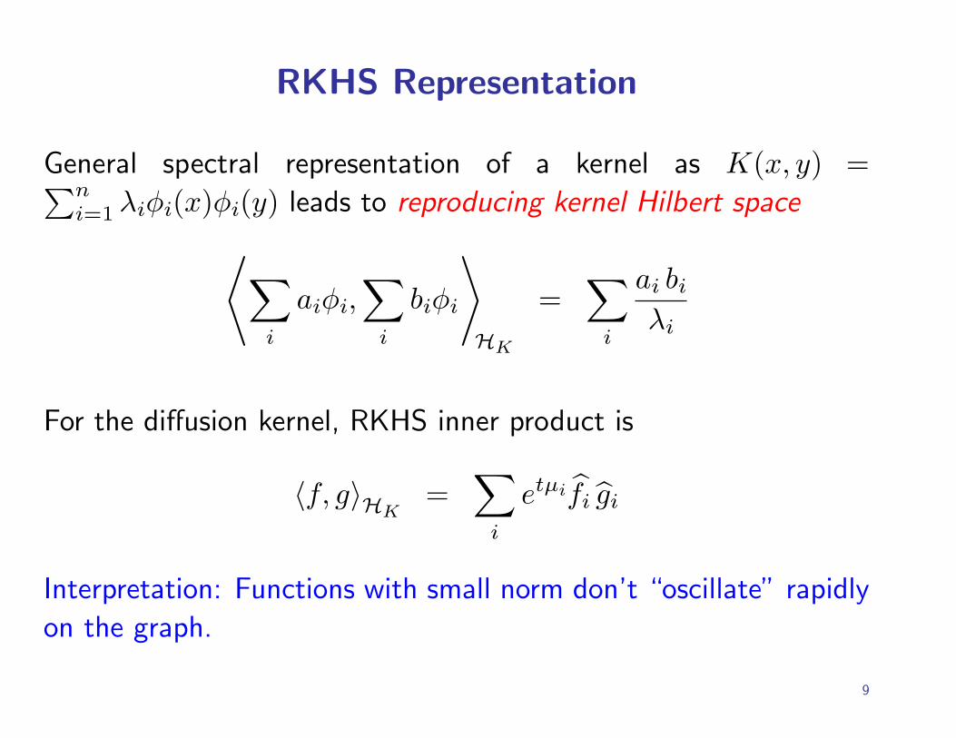
RKHS Representation
General spectral representation of a kernel as K(x, y) =∑ni=1 λiφi(x)φi(y) leads to reproducing kernel Hilbert space
⟨∑
i
aiφi,∑
i
biφi
⟩
HK
=∑
i
ai bi
λi
For the diffusion kernel, RKHS inner product is
〈f, g〉HK=
∑
i
etµifi gi
Interpretation: Functions with small norm don’t “oscillate” rapidly
on the graph.
9
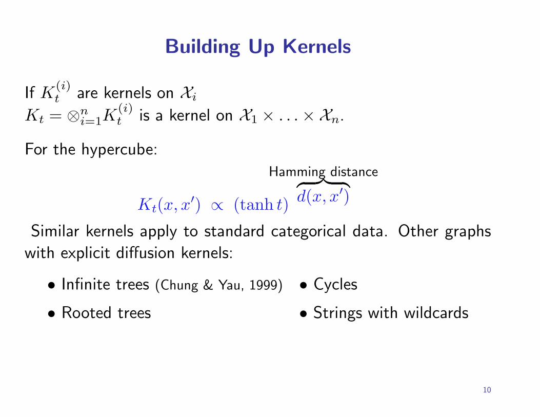
Building Up Kernels
If K(i)t are kernels on Xi
Kt = ⊗ni=1K
(i)t is a kernel on X1 × . . .×Xn.
For the hypercube:
Kt(x, x′) ∝ (tanh t)
Hamming distance︷ ︸︸ ︷d(x, x′)
Similar kernels apply to standard categorical data. Other graphs
with explicit diffusion kernels:
• Infinite trees (Chung & Yau, 1999) • Cycles
• Rooted trees • Strings with wildcards
10
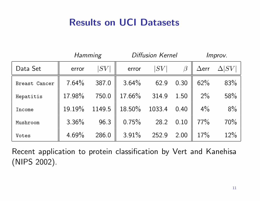
Results on UCI Datasets
Hamming Diffusion Kernel Improv.
Data Set error |SV | error |SV | β ∆err ∆|SV |Breast Cancer 7.64% 387.0 3.64% 62.9 0.30 62% 83%
Hepatitis 17.98% 750.0 17.66% 314.9 1.50 2% 58%
Income 19.19% 1149.5 18.50% 1033.4 0.40 4% 8%
Mushroom 3.36% 96.3 0.75% 28.2 0.10 77% 70%
Votes 4.69% 286.0 3.91% 252.9 2.00 17% 12%
Recent application to protein classification by Vert and Kanehisa
(NIPS 2002).
11
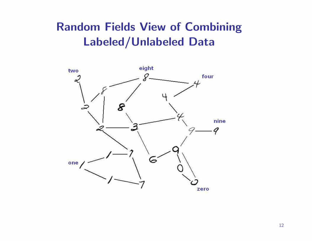
Random Fields View of CombiningLabeled/Unlabeled Data
12
Random Fields View
View each vertex x as having label f(x) ∈ {+1,−1}.Ising model on graph/lattice, spins f : V −→ {+1,−1}
Energy H(f) =12
∑x∼y
wxy (f(x)− f(y))2
≡ −∑x∼y
wxyf(x) f(y)
Gibbs distribution P (f) =1
Z(β)e−βH(f) β =
1T
Partition function Z(β) =∑
f
e−βH(f)
13
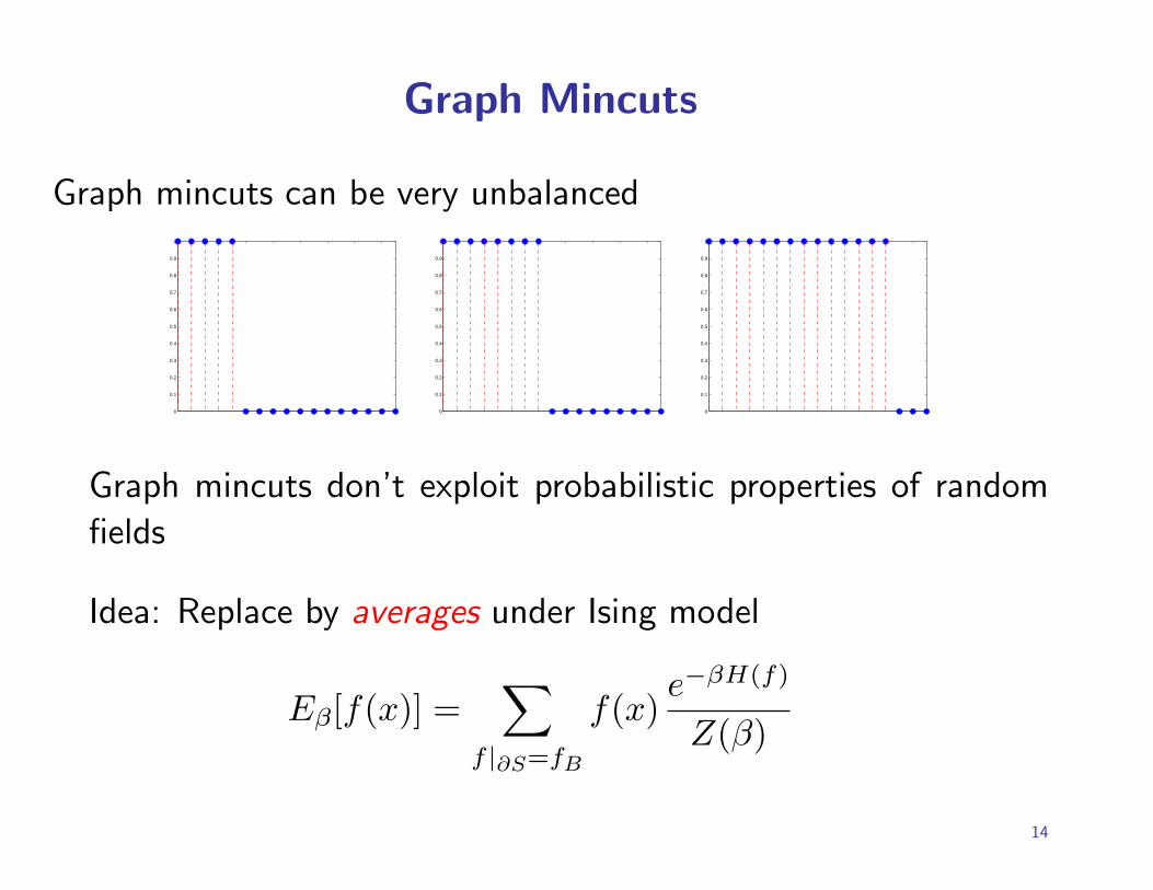
Graph Mincuts
Graph mincuts can be very unbalanced
0
0.1
0.2
0.3
0.4
0.5
0.6
0.7
0.8
0.9
1
0
0.1
0.2
0.3
0.4
0.5
0.6
0.7
0.8
0.9
1
0
0.1
0.2
0.3
0.4
0.5
0.6
0.7
0.8
0.9
1
Graph mincuts don’t exploit probabilistic properties of random
fields
Idea: Replace by averages under Ising model
Eβ[f(x)] =∑
f |∂S=fB
f(x)e−βH(f)
Z(β)
14
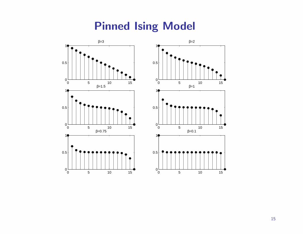
Pinned Ising Model
0 5 10 150
0.5
1β=3
0 5 10 150
0.5
1β=2
0 5 10 150
0.5
1β=1.5
0 5 10 150
0.5
1β=1
0 5 10 150
0.5
1β=0.75
0 5 10 150
0.5
1β=0.1
15
Not (Provably) Efficient to Approximate
Unfortunately, analogue of rapid mixing result of Jerrum & Sinclair
for ferromagnetic Ising model not known for mixed boundary
conditions
Question: Can we compute averages using graph algorithms in the
zero temperature limit?
16
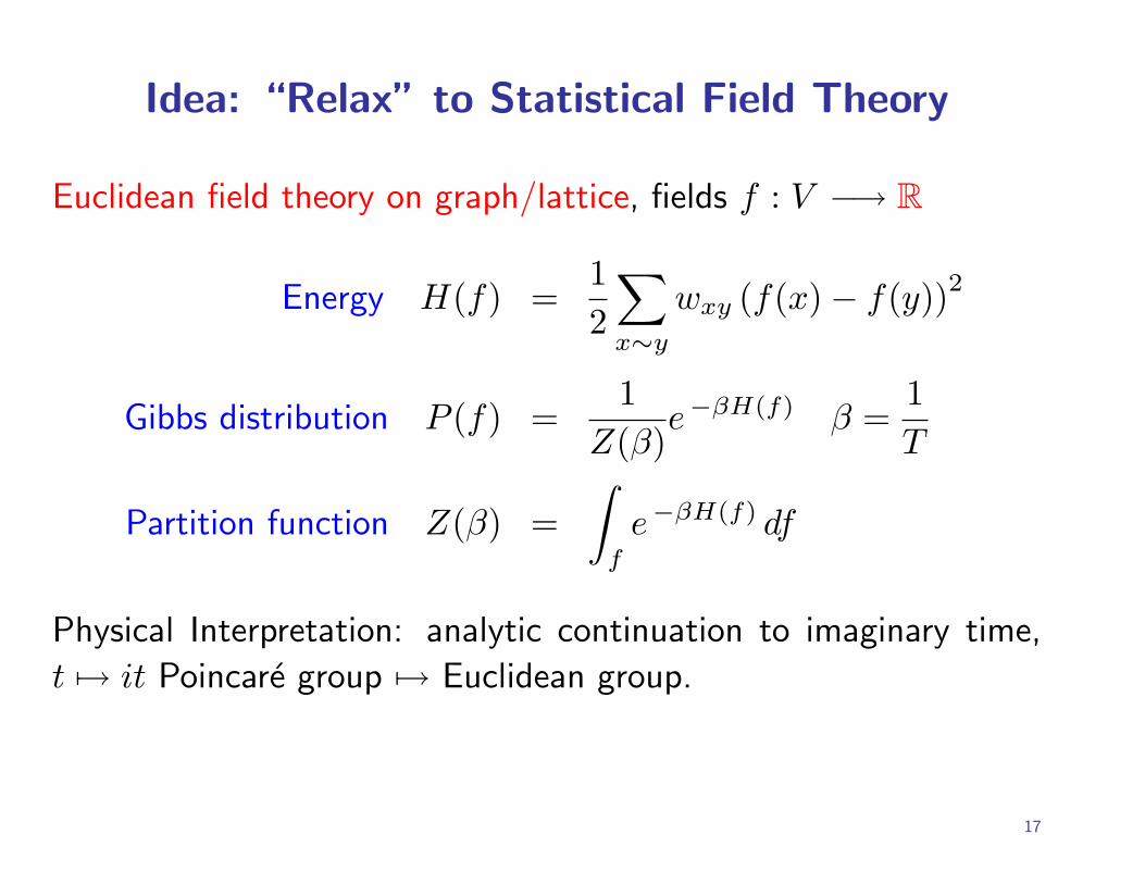
Idea: “Relax” to Statistical Field Theory
Euclidean field theory on graph/lattice, fields f : V −→ R
Energy H(f) =12
∑x∼y
wxy (f(x)− f(y))2
Gibbs distribution P (f) =1
Z(β)e−βH(f) β =
1T
Partition function Z(β) =∫
f
e−βH(f) df
Physical Interpretation: analytic continuation to imaginary time,
t 7→ it Poincare group 7→ Euclidean group.
17
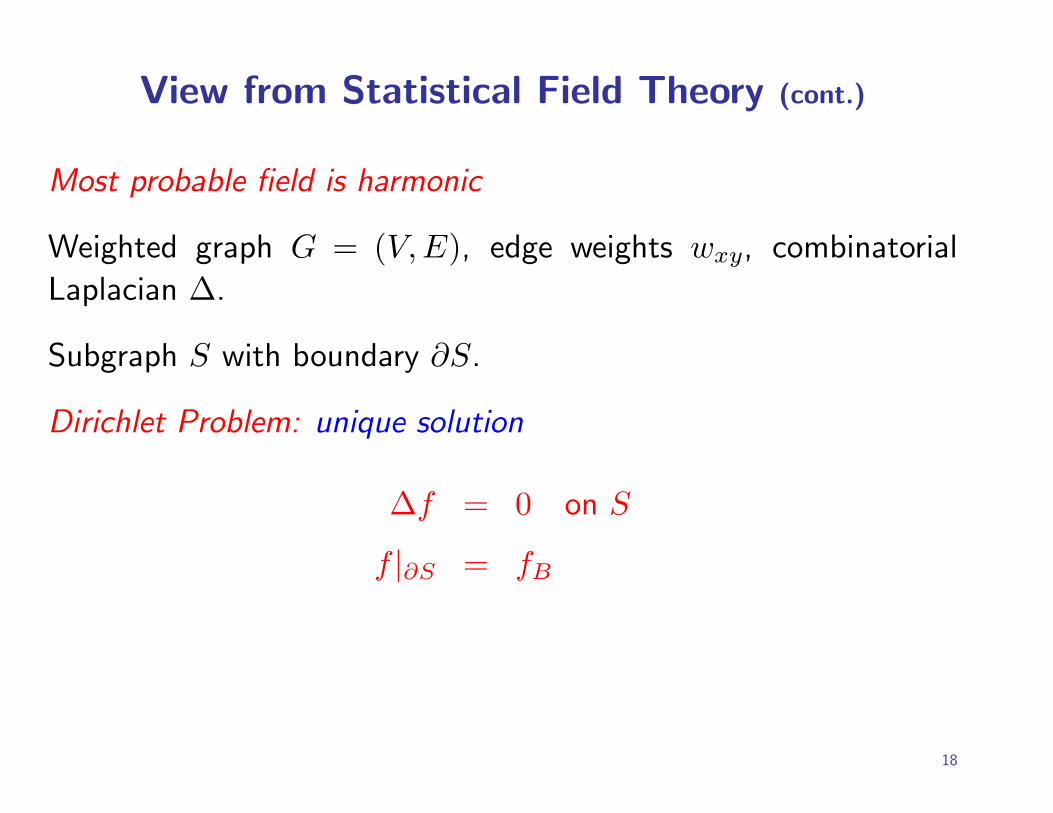
View from Statistical Field Theory (cont.)
Most probable field is harmonic
Weighted graph G = (V, E), edge weights wxy, combinatorial
Laplacian ∆.
Subgraph S with boundary ∂S.
Dirichlet Problem: unique solution
∆f = 0 on S
f |∂S = fB
18
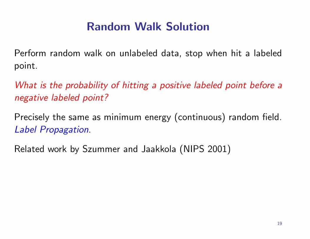
Random Walk Solution
Perform random walk on unlabeled data, stop when hit a labeled
point.
What is the probability of hitting a positive labeled point before a
negative labeled point?
Precisely the same as minimum energy (continuous) random field.
Label Propagation.
Related work by Szummer and Jaakkola (NIPS 2001)
19
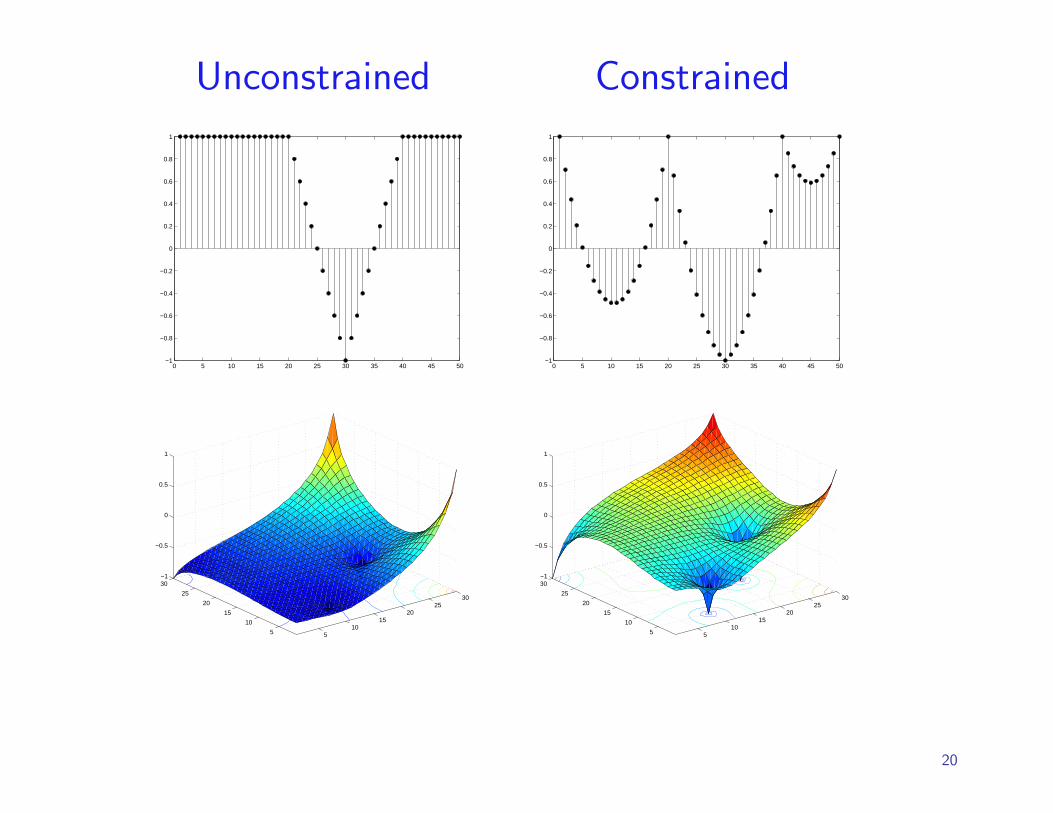
Unconstrained Constrained
0 5 10 15 20 25 30 35 40 45 50−1
−0.8
−0.6
−0.4
−0.2
0
0.2
0.4
0.6
0.8
1
0 5 10 15 20 25 30 35 40 45 50−1
−0.8
−0.6
−0.4
−0.2
0
0.2
0.4
0.6
0.8
1
510
1520
2530
5
10
15
20
25
30−1
−0.5
0
0.5
1
510
1520
2530
5
10
15
20
25
30−1
−0.5
0
0.5
1
20
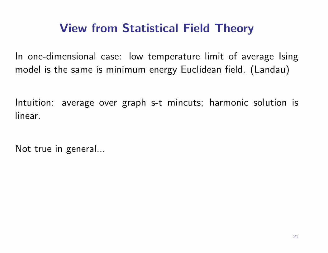
View from Statistical Field Theory
In one-dimensional case: low temperature limit of average Ising
model is the same is minimum energy Euclidean field. (Landau)
Intuition: average over graph s-t mincuts; harmonic solution is
linear.
Not true in general...
21
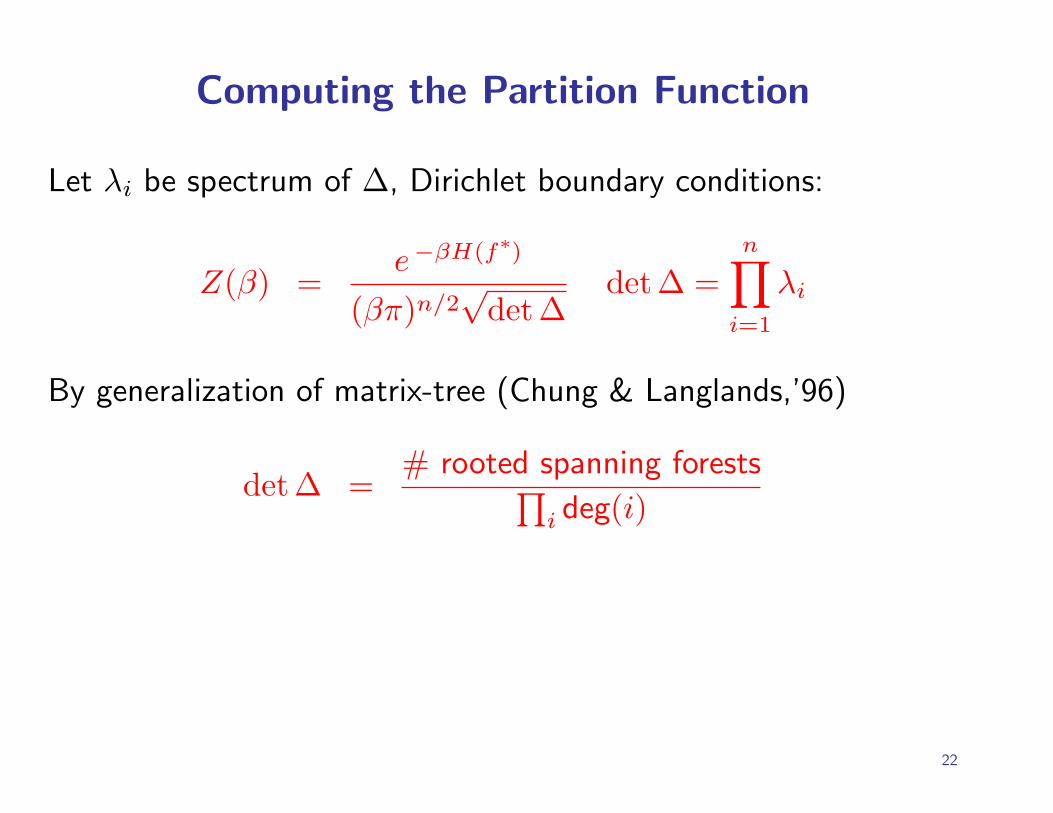
Computing the Partition Function
Let λi be spectrum of ∆, Dirichlet boundary conditions:
Z(β) =e−βH(f∗)
(βπ)n/2√
det∆det∆ =
n∏
i=1
λi
By generalization of matrix-tree (Chung & Langlands,’96)
det∆ =# rooted spanning forests∏
i deg(i)
22
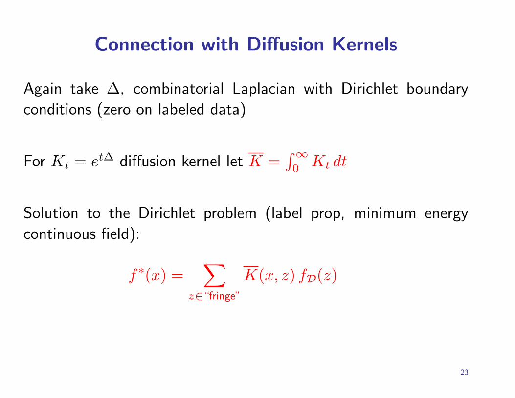
Connection with Diffusion Kernels
Again take ∆, combinatorial Laplacian with Dirichlet boundary
conditions (zero on labeled data)
For Kt = et∆ diffusion kernel let K =∫∞0
Kt dt
Solution to the Dirichlet problem (label prop, minimum energy
continuous field):
f∗(x) =∑
z∈“fringe”
K(x, z) fD(z)
23
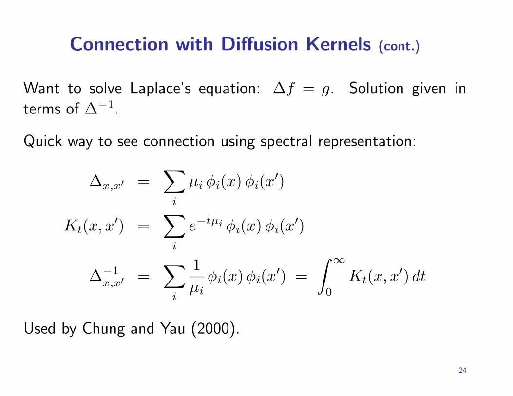
Connection with Diffusion Kernels (cont.)
Want to solve Laplace’s equation: ∆f = g. Solution given in
terms of ∆−1.
Quick way to see connection using spectral representation:
∆x,x′ =∑
i
µi φi(x) φi(x′)
Kt(x, x′) =∑
i
e−tµi φi(x)φi(x′)
∆−1x,x′ =
∑
i
1µi
φi(x) φi(x′) =∫ ∞
0
Kt(x, x′) dt
Used by Chung and Yau (2000).
24
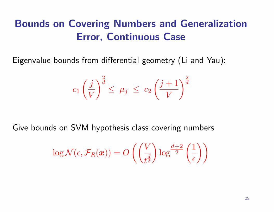
Bounds on Covering Numbers and GeneralizationError, Continuous Case
Eigenvalue bounds from differential geometry (Li and Yau):
c1
(j
V
)2d
≤ µj ≤ c2
(j + 1
V
)2d
Give bounds on SVM hypothesis class covering numbers
logN (ε,FR(x)) = O
((V
td2
)log
d+22
(1ε
))
25
Bounds on Generalization Error
Better bounds on generalization error are now available based
on Rademacher averages involving trace of the kernel (Bartlett,
Bousquet, & Mendelson, preprint).
Question: Can diffusion kernel connection be exploited to
get transductive generalization error bounds for random walks
approach?
26
Summary
Random fields with discrete class labels—intractable, unstable
Continuous fields—tractable, more desirable behavior for
segentation and labeling
Intimate connections with random walks, electric networks,
graph flows, and diffusion kernels
Advantages/disadvantages?
27


![COVER TIMES FOR BROWNIAN MOTION AND … · arXiv:math/0107191v2 [math.PR] 27 Nov 2003 COVER TIMES FOR BROWNIAN MOTION AND RANDOM WALKS IN TWO DIMENSIONS AMIR DEMBO∗ YUVAL PERES†](https://static.fdocument.org/doc/165x107/5e7ac976afe2e26c446aa64f/cover-times-for-brownian-motion-and-arxivmath0107191v2-mathpr-27-nov-2003-cover.jpg)