Ross B 13dec'10 8mar'11 009-AR ver.3 : Stainless Steel vs. Copper Dipole Comparison Page 1 of 6

Tech. Rept. 009 – AR

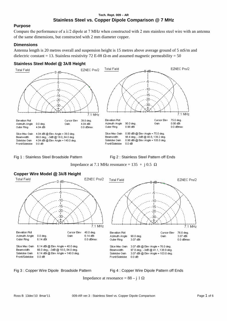
Stainless Steel vs. Copper Dipole Comparison @ 7 MHz Purpose Compare the performance of a λ/2 dipole at 7 MHz when constructed with 2 mm stainless steel wire with an antenna of the same dimensions, but constructed with 2 mm diameter copper.

Dimensions Antenna length is 20 metres overall and suspension height is 15 metres above average ground of 5 mS/m and dielectric constant = 13. Stainless resistivity 72 E-08 Ω-m and assumed magnetic permeability = 50

Stainless Steel Model @ 3λ/8 Height

Fig 1 : Stainless Steel Broadside Pattern Fig 2 : Stainless Steel Pattern off Ends

Impedance at 7.1 MHz resonance = 135 + j 0.5 Ω

Copper Wire Model @ 3λ/8 Height

Fig 3 : Copper Wire Dipole Broadside Pattern Fig 4 : Copper Wire Dipole Pattern off Ends

Impedance at resonance = 88 – j 1 Ω

Ross B 13dec'10 8mar'11 009-AR ver.3 : Stainless Steel vs. Copper Dipole Comparison Page 2 of 6

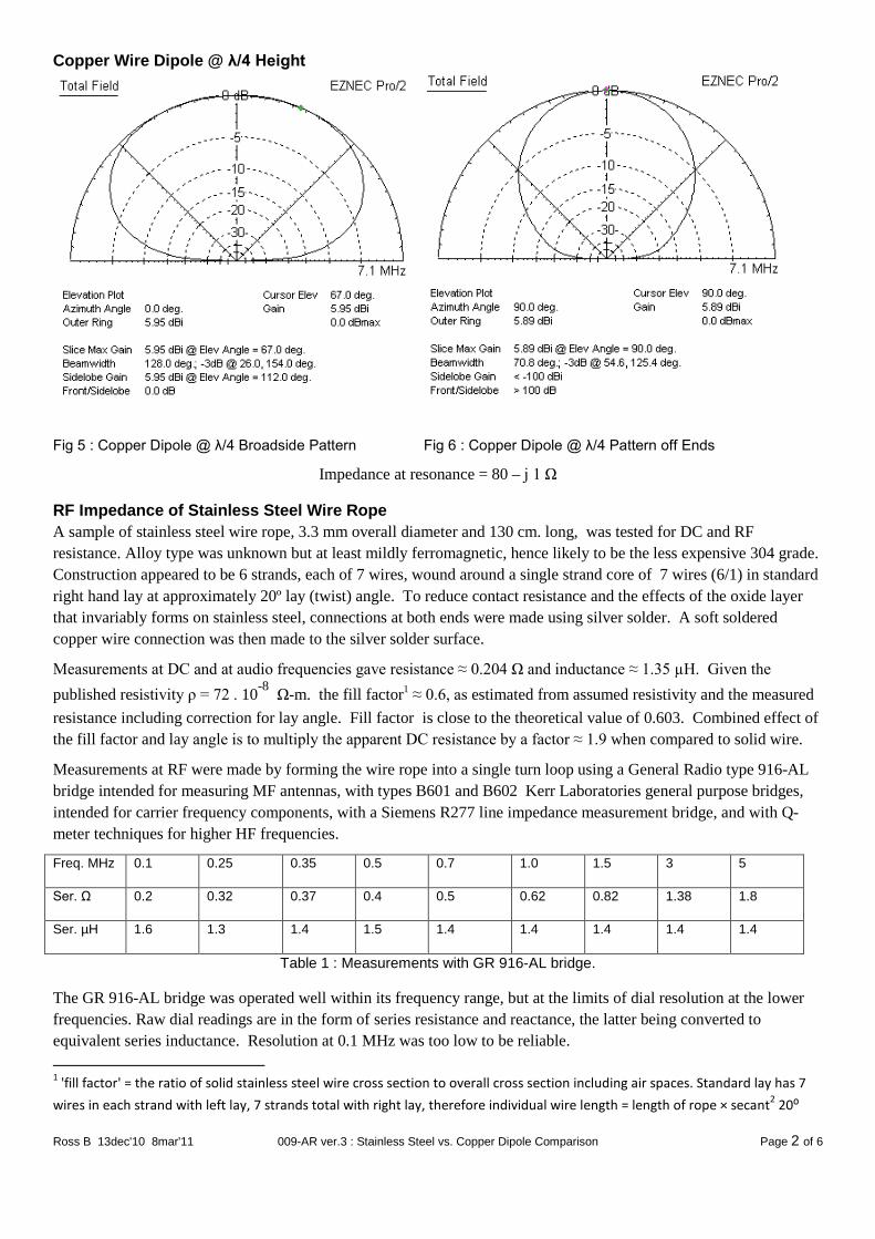
Copper Wire Dipole @ λ/4 Height

Fig 5 : Copper Dipole @ λ/4 Broadside Pattern Fig 6 : Copper Dipole @ λ/4 Pattern off Ends

Impedance at resonance = 80 – j 1 Ω

RF Impedance of Stainless Steel Wire Rope A sample of stainless steel wire rope, 3.3 mm overall diameter and 130 cm. long, was tested for DC and RF resistance. Alloy type was unknown but at least mildly ferromagnetic, hence likely to be the less expensive 304 grade. Construction appeared to be 6 strands, each of 7 wires, wound around a single strand core of 7 wires (6/1) in standard right hand lay at approximately 20º lay (twist) angle. To reduce contact resistance and the effects of the oxide layer that invariably forms on stainless steel, connections at both ends were made using silver solder. A soft soldered copper wire connection was then made to the silver solder surface.

Measurements at DC and at audio frequencies gave resistance ≈ 0.204 Ω and inductance ≈ 1.35 µH. Given the published resistivity ρ = 72 . 10-8 Ω-m. the fill factor1 ≈ 0.6, as estimated from assumed resistivity and the measured resistance including correction for lay angle. Fill factor is close to the theoretical value of 0.603. Combined effect of the fill factor and lay angle is to multiply the apparent DC resistance by a factor ≈ 1.9 when compared to solid wire.

Measurements at RF were made by forming the wire rope into a single turn loop using a General Radio type 916-AL bridge intended for measuring MF antennas, with types B601 and B602 Kerr Laboratories general purpose bridges, intended for carrier frequency components, with a Siemens R277 line impedance measurement bridge, and with Q-meter techniques for higher HF frequencies.

Freq. MHz 0.1 0.25 0.35 0.5 0.7 1.0 1.5 3 5

Ser. Ω 0.2 0.32 0.37 0.4 0.5 0.62 0.82 1.38 1.8

Ser. µH 1.6 1.3 1.4 1.5 1.4 1.4 1.4 1.4 1.4

Table 1 : Measurements with GR 916-AL bridge.

The GR 916-AL bridge was operated well within its frequency range, but at the limits of dial resolution at the lower frequencies. Raw dial readings are in the form of series resistance and reactance, the latter being converted to equivalent series inductance. Resolution at 0.1 MHz was too low to be reliable. 1 'fill factor' = the ratio of solid stainless steel wire cross section to overall cross section including air spaces. Standard lay has 7 wires in each strand with left lay, 7 strands total with right lay, therefore individual wire length = length of rope × secant2 20⁰

Ross B 13dec'10 8mar'11 009-AR ver.3 : Stainless Steel vs. Copper Dipole Comparison Page 3 of 6

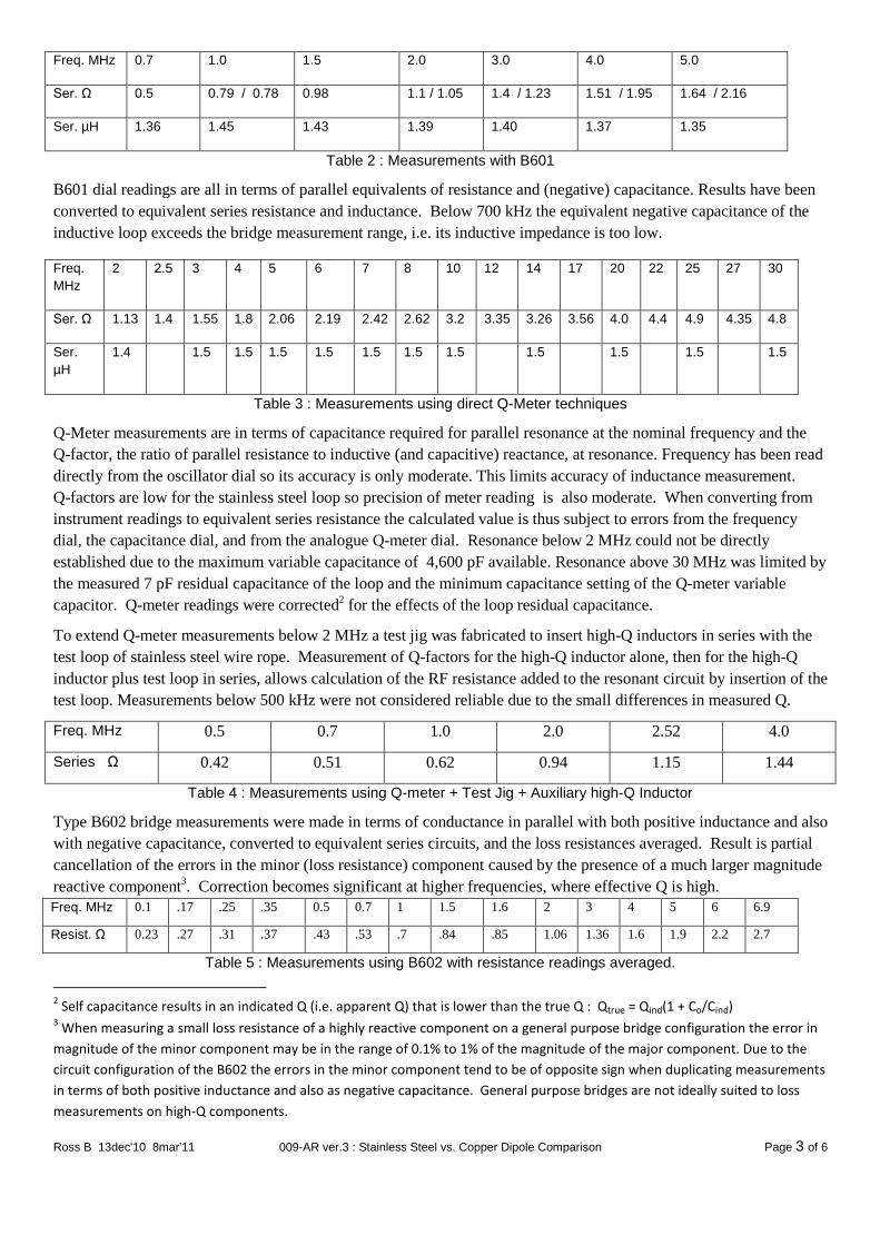
Freq. MHz 0.7 1.0 1.5 2.0 3.0 4.0 5.0

Ser. Ω 0.5 0.79 / 0.78 0.98 1.1 / 1.05 1.4 / 1.23 1.51 / 1.95 1.64 / 2.16

Ser. µH 1.36 1.45 1.43 1.39 1.40 1.37 1.35

Table 2 : Measurements with B601

B601 dial readings are all in terms of parallel equivalents of resistance and (negative) capacitance. Results have been converted to equivalent series resistance and inductance. Below 700 kHz the equivalent negative capacitance of the inductive loop exceeds the bridge measurement range, i.e. its inductive impedance is too low.

Freq. MHz

2 2.5 3 4 5 6 7 8 10 12 14 17 20 22 25 27 30

Ser. Ω 1.13 1.4 1.55 1.8 2.06 2.19 2.42 2.62 3.2 3.35 3.26 3.56 4.0 4.4 4.9 4.35 4.8

Ser. µH

1.4 1.5 1.5 1.5 1.5 1.5 1.5 1.5 1.5 1.5 1.5 1.5

Table 3 : Measurements using direct Q-Meter techniques

Q-Meter measurements are in terms of capacitance required for parallel resonance at the nominal frequency and the Q-factor, the ratio of parallel resistance to inductive (and capacitive) reactance, at resonance. Frequency has been read directly from the oscillator dial so its accuracy is only moderate. This limits accuracy of inductance measurement. Q-factors are low for the stainless steel loop so precision of meter reading is also moderate. When converting from instrument readings to equivalent series resistance the calculated value is thus subject to errors from the frequency dial, the capacitance dial, and from the analogue Q-meter dial. Resonance below 2 MHz could not be directly established due to the maximum variable capacitance of 4,600 pF available. Resonance above 30 MHz was limited by the measured 7 pF residual capacitance of the loop and the minimum capacitance setting of the Q-meter variable capacitor. Q-meter readings were corrected2 for the effects of the loop residual capacitance.

To extend Q-meter measurements below 2 MHz a test jig was fabricated to insert high-Q inductors in series with the test loop of stainless steel wire rope. Measurement of Q-factors for the high-Q inductor alone, then for the high-Q inductor plus test loop in series, allows calculation of the RF resistance added to the resonant circuit by insertion of the test loop. Measurements below 500 kHz were not considered reliable due to the small differences in measured Q.

Freq. MHz 0.5 0.7 1.0 2.0 2.52 4.0

Series Ω 0.42 0.51 0.62 0.94 1.15 1.44

Table 4 : Measurements using Q-meter + Test Jig + Auxiliary high-Q Inductor

Type B602 bridge measurements were made in terms of conductance in parallel with both positive inductance and also with negative capacitance, converted to equivalent series circuits, and the loss resistances averaged. Result is partial cancellation of the errors in the minor (loss resistance) component caused by the presence of a much larger magnitude reactive component3. Correction becomes significant at higher frequencies, where effective Q is high. Freq. MHz 0.1 .17 .25 .35 0.5 0.7 1 1.5 1.6 2 3 4 5 6 6.9

Resist. Ω 0.23 .27 .31 .37 .43 .53 .7 .84 .85 1.06 1.36 1.6 1.9 2.2 2.7

Table 5 : Measurements using B602 with resistance readings averaged. 2 Self capacitance results in an indicated Q (i.e. apparent Q) that is lower than the true Q : Qtrue = Qind(1 + Co/Cind) 3 When measuring a small loss resistance of a highly reactive component on a general purpose bridge configuration the error in magnitude of the minor component may be in the range of 0.1% to 1% of the magnitude of the major component. Due to the circuit configuration of the B602 the errors in the minor component tend to be of opposite sign when duplicating measurements in terms of both positive inductance and also as negative capacitance. General purpose bridges are not ideally suited to loss measurements on high-Q components.

Ross B 13dec'10 8mar'11 009-AR ver.3 : Stainless Steel vs. Copper Dipole Comparison Page 4 of 6

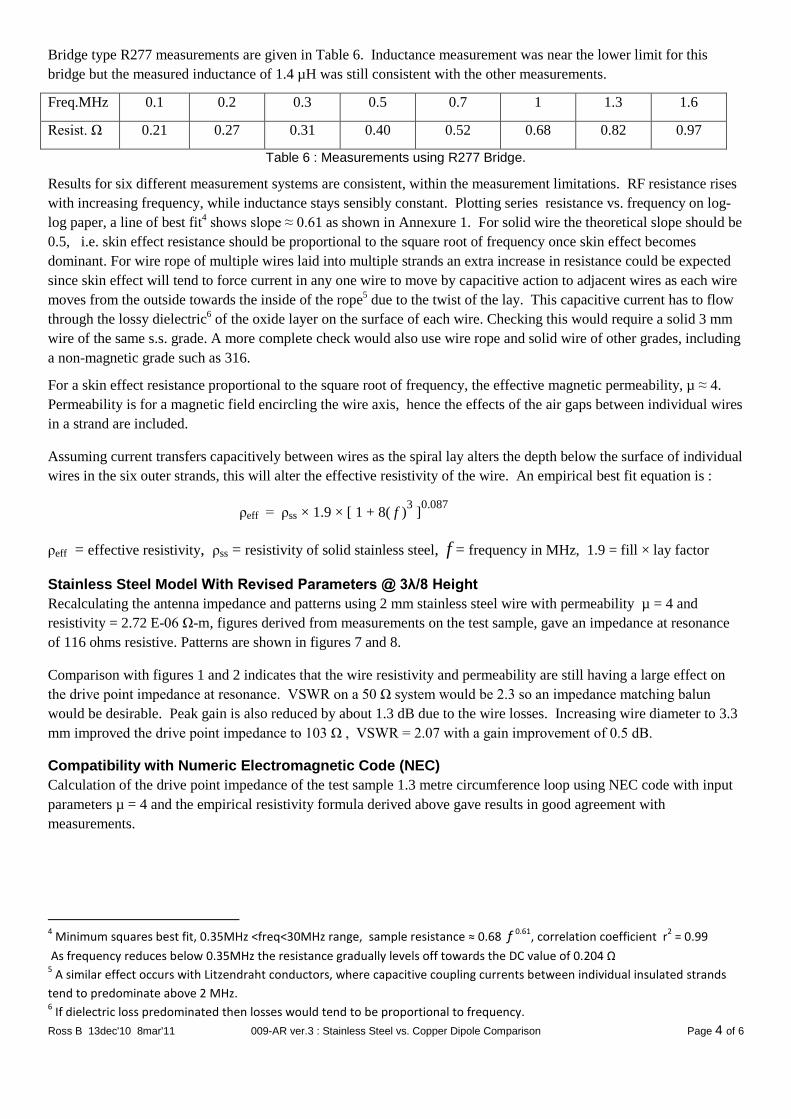
Bridge type R277 measurements are given in Table 6. Inductance measurement was near the lower limit for this bridge but the measured inductance of 1.4 µH was still consistent with the other measurements.

Freq.MHz 0.1 0.2 0.3 0.5 0.7 1 1.3 1.6

Resist. Ω 0.21 0.27 0.31 0.40 0.52 0.68 0.82 0.97

Table 6 : Measurements using R277 Bridge.

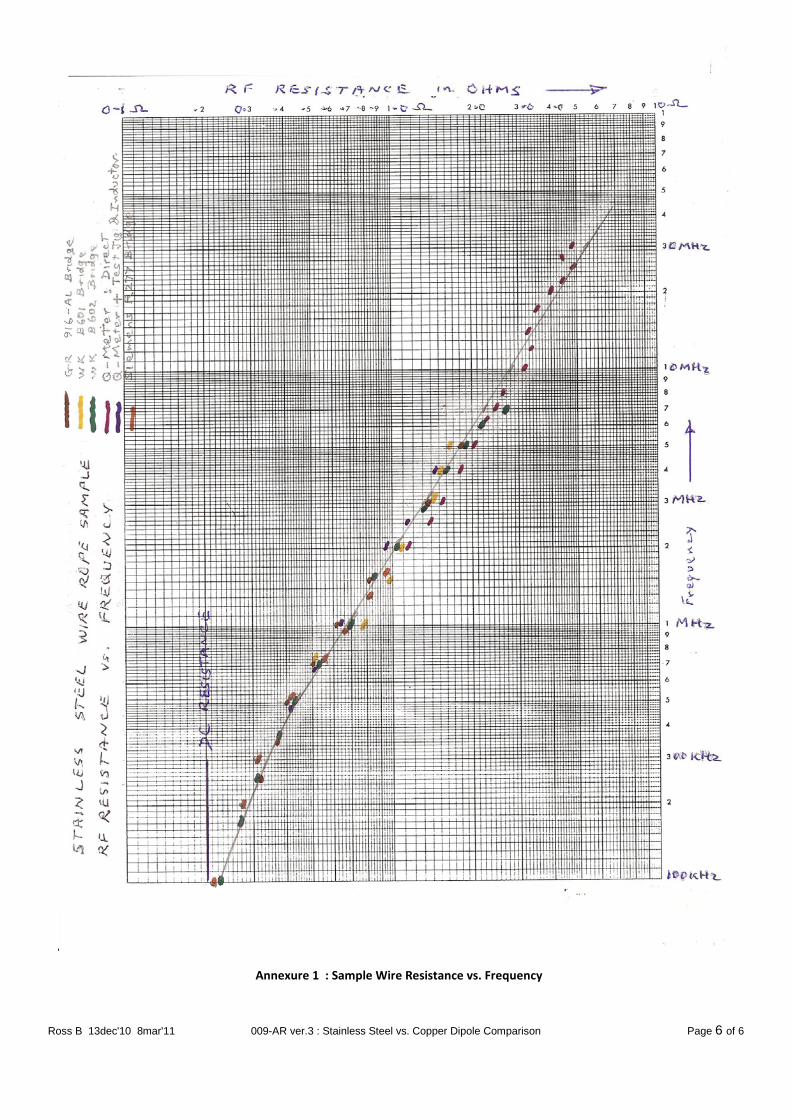
Results for six different measurement systems are consistent, within the measurement limitations. RF resistance rises with increasing frequency, while inductance stays sensibly constant. Plotting series resistance vs. frequency on log-log paper, a line of best fit4 shows slope ≈ 0.61 as shown in Annexure 1. For solid wire the theoretical slope should be 0.5, i.e. skin effect resistance should be proportional to the square root of frequency once skin effect becomes dominant. For wire rope of multiple wires laid into multiple strands an extra increase in resistance could be expected since skin effect will tend to force current in any one wire to move by capacitive action to adjacent wires as each wire moves from the outside towards the inside of the rope5 due to the twist of the lay. This capacitive current has to flow through the lossy dielectric6 of the oxide layer on the surface of each wire. Checking this would require a solid 3 mm wire of the same s.s. grade. A more complete check would also use wire rope and solid wire of other grades, including a non-magnetic grade such as 316.

For a skin effect resistance proportional to the square root of frequency, the effective magnetic permeability, µ ≈ 4. Permeability is for a magnetic field encircling the wire axis, hence the effects of the air gaps between individual wires in a strand are included.

Assuming current transfers capacitively between wires as the spiral lay alters the depth below the surface of individual wires in the six outer strands, this will alter the effective resistivity of the wire. An empirical best fit equation is :

ρeff = ρss × 1.9 × [ 1 + 8( f )3 ]0.087

ρeff = effective resistivity, ρss = resistivity of solid stainless steel, f = frequency in MHz, 1.9 = fill × lay factor

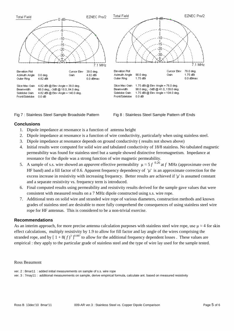
Stainless Steel Model With Revised Parameters @ 3λ/8 Height Recalculating the antenna impedance and patterns using 2 mm stainless steel wire with permeability µ = 4 and resistivity = 2.72 E-06 Ω-m, figures derived from measurements on the test sample, gave an impedance at resonance of 116 ohms resistive. Patterns are shown in figures 7 and 8.

Comparison with figures 1 and 2 indicates that the wire resistivity and permeability are still having a large effect on the drive point impedance at resonance. VSWR on a 50 Ω system would be 2.3 so an impedance matching balun would be desirable. Peak gain is also reduced by about 1.3 dB due to the wire losses. Increasing wire diameter to 3.3 mm improved the drive point impedance to 103 Ω , VSWR = 2.07 with a gain improvement of 0.5 dB.

Compatibility with Numeric Electromagnetic Code (NEC) Calculation of the drive point impedance of the test sample 1.3 metre circumference loop using NEC code with input parameters µ = 4 and the empirical resistivity formula derived above gave results in good agreement with measurements.

4 Minimum squares best fit, 0.35MHz <freq<30MHz range, sample resistance ≈ 0.68 f 0.61, correlation coefficient r2 = 0.99 As frequency reduces below 0.35MHz the resistance gradually levels off towards the DC value of 0.204 Ω 5 A similar effect occurs with Litzendraht conductors, where capacitive coupling currents between individual insulated strands tend to predominate above 2 MHz. 6 If dielectric loss predominated then losses would tend to be proportional to frequency.

Ross B 13dec'10 8mar'11 009-AR ver.3 : Stainless Steel vs. Copper Dipole Comparison Page 5 of 6

Fig 7 : Stainless Steel Sample Broadside Pattern Fig 8 : Stainless Steel Sample Pattern off Ends

Conclusions 1. Dipole impedance at resonance is a function of antenna height 2. Dipole impedance at resonance is a function of wire conductivity, particularly when using stainless steel. 3. Dipole impedance at resonance depends on ground conductivity ( results not shown above) 4. Initial results were computed for solid wire and tabulated conductivity of 18/8 stainless. No tabulated magnetic

permeability was found for stainless steel but a sample showed distinctive ferromagnetism. Impedance at resonance for the dipole was a strong function of wire magnetic permeability.

5. A sample of s.s. wire showed an apparent effective permeability µ ≈ 5 f 0.26 at f MHz (approximate over the HF band) and a fill factor of 0.6. Apparent frequency dependency of 'µ' is an approximate correction for the excess increase in resistivity with increasing frequency. Better results are achieved if 'µ' is assumed constant and a separate resistivity vs. frequency term is introduced.

6. Final computed results using permeability and resistivity results derived for the sample gave values that were consistent with measured results on a 7 MHz dipole constructed using s.s. wire rope.

7. Additional tests on solid wire and stranded wire rope of various diameters, construction methods and known grades of stainless steel are desirable to more fully comprehend the consequences of using stainless steel wire rope for HF antennas. This is considered to be a non-trivial exercise.

Recommendations As an interim approach, for more precise antenna calculation purposes with stainless steel wire rope, use µ ≈ 4 for skin effect calculations, multiply resistivity by 1.9 to allow for fill factor and lay angle of the wires comprising the stranded rope, and by [ 1 + 8( f )3 ]0.087 to allow for the additional frequency dependent losses . These values are empirical : they apply to the particular grade of stainless steel and the type of wire lay used for the sample tested.

Ross Beaumont

ver. 2 : 8mar11 : added initial measurements on sample of s.s. wire rope ver. 3 : 7may11 : additional measurements on sample, derive empirical formula, calculate ant. based on measured resistivity

Ross B 13dec'10 8mar'11 009-AR ver.3 : Stainless Steel vs. Copper Dipole Comparison Page 6 of 6

Annexure 1 : Sample Wire Resistance vs. Frequency