Higher-order Fourier Analysis over Finite Fields,and Applications

Pooya Hatami

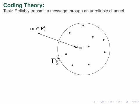
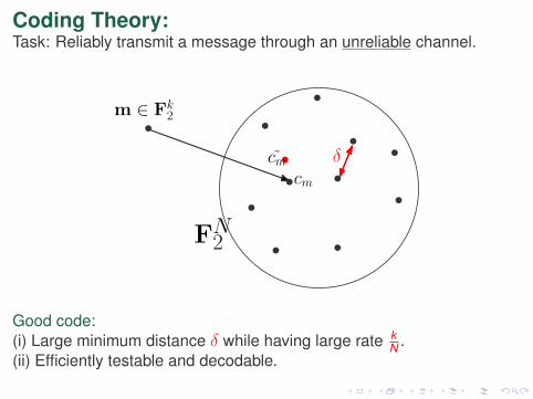
Coding Theory:Task: Reliably transmit a message through an unreliable channel.

m ∈ Fk2

FN2

cm

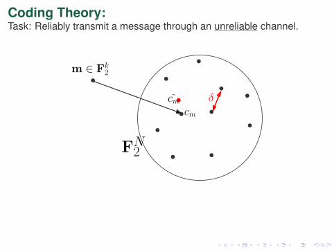
Coding Theory:Task: Reliably transmit a message through an unreliable channel.

m ∈ Fk2

FN2

cm

δc̃m

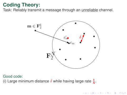
Coding Theory:Task: Reliably transmit a message through an unreliable channel.

m ∈ Fk2

FN2

cm

δc̃m

Good code:(i) Large minimum distance δ while having large rate k

N .

Coding Theory:Task: Reliably transmit a message through an unreliable channel.

m ∈ Fk2

FN2

cm

δc̃m

Good code:(i) Large minimum distance δ while having large rate k

N .(ii) Efficiently testable and decodable.

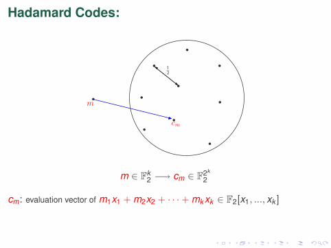
Hadamard Codes:

12

cm

m

m ∈ Fk2 −→ cm ∈ F2k

2

cm: evaluation vector of m1x1 + m2x2 + · · ·+ mkxk ∈ F2[x1, ..., xk ]

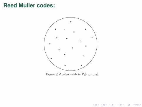
Reed Muller codes:

Degree ≤ d polynomials in F2[x1, ..., xk]

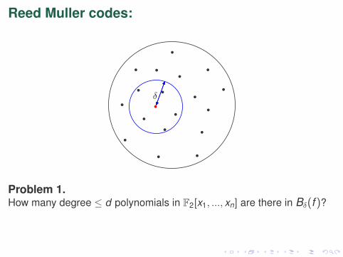
Reed Muller codes:

δ

Problem 1.How many degree ≤ d polynomials in F2[x1, ..., xn] are there in Bδ(f )?

Polynomial Decompositions:

Degree 4 polynomial P ∈ F2[x1, ..., xn].

Is

P(x) = Q1(x)Q2(x) + Q3(x)Q4(x),

for some degree ≤ 3 polynomials Q1, ...,Q4?

Polynomial Decompositions:

Degree 4 polynomial P ∈ F2[x1, ..., xn]. Is

P(x) = Q1(x)Q2(x) + Q3(x)Q4(x),

for some degree ≤ 3 polynomials Q1, ...,Q4?

Polynomial Decompositions:

Degree 4 polynomial P ∈ F2[x1, ..., xn]. Is

P(x) = Q1(x)Q2(x) + Q3(x)Q4(x),

for some degree ≤ 3 polynomials Q1, ...,Q4?

Problem 2.Given a degree d polynomial P and a prescribed decomposition.Find such a decomposition of P or say it is not possible.

Polynomial Decompositions:

Degree 4 polynomial P ∈ F2[x1, ..., xn]. Is

P(x) = Q1(x)Q2(x) + Q3(x)Q4(x),

for some degree ≤ 3 polynomials Q1, ...,Q4?

Problem 2.Given a degree d polynomial P and a prescribed decomposition,Efficiently find such a decomposition of P or say it is not possible.

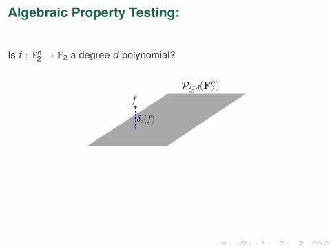
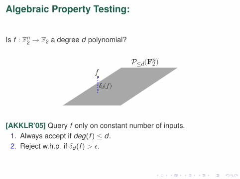
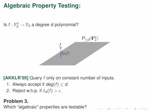
Algebraic Property Testing:

Is f : Fn2 → F2 a degree d polynomial?

f

P≤d(Fn2 )

δd(f )

[AKKLR’05] Query f only on constant number of inputs.1. Always accept if deg(f ) ≤ d .2. Reject w.h.p. if δd (f ) > ε.

Problem 3.Which “algebraic” properties are testable?

Algebraic Property Testing:

Is f : Fn2 → F2 a degree d polynomial?

f

P≤d(Fn2 )

δd(f )

[AKKLR’05] Query f only on constant number of inputs.1. Always accept if deg(f ) ≤ d .2. Reject w.h.p. if δd (f ) > ε.

Problem 3.Which “algebraic” properties are testable?

Algebraic Property Testing:

Is f : Fn2 → F2 a degree d polynomial?

f

P≤d(Fn2 )

δd(f )

[AKKLR’05] Query f only on constant number of inputs.1. Always accept if deg(f ) ≤ d .2. Reject w.h.p. if δd (f ) > ε.

Problem 3.Which “algebraic” properties are testable?

Higher-order Fourier analysis over finite fields,which is an extension of Fourier analysis.

[Bergelson, Green, Kaufman, Gowers, Lovett, Meshulam, Samorodnitsky, Tao, Viola, Wolf . . . ]

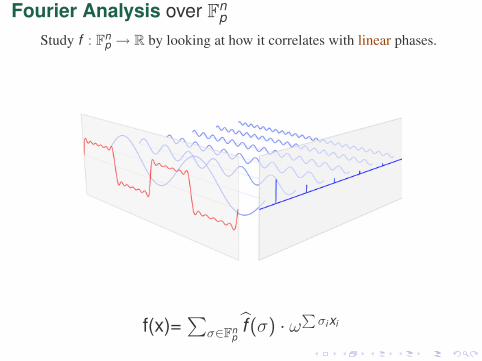
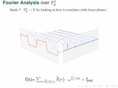
Fourier Analysis over Fnp

Study f : Fnp → R by looking at how it correlates with linear phases.

f(x)=∑

σ∈Fnpf̂ (σ) · ω

∑σixi

Fourier Analysis over Fnp

Study f : Fnp → R by looking at how it correlates with linear phases.

f(x)=∑

σ:|̂f (σ)|≥ε f̂ (σ) · ω∑σixi + fpsd

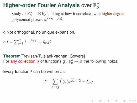
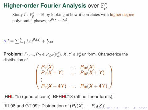
Higher-order Fourier Analysis over Fnp

Study f : Fnp → R by looking at how it correlates with higher degree

polynomial phases, ωP(x1,...,xn).

� Not orthogonal, no unique expansion.

� f =∑C

i=1 λiωPi (x) + fpsd?

Higher-order Fourier Analysis over Fnp

Study f : Fnp → R by looking at how it correlates with higher degree

polynomial phases, ωP(x1,...,xn).

� Not orthogonal, no unique expansion.

� f =∑C

i=1 λiωPi (x) + fpsd?

[Bergelson, Green, Tao, Ziegler] establish such decompositiontheorems via inverse theorems for certain norms called Gowers norms.

Higher-order Fourier Analysis over Fnp

Study f : Fnp → R by looking at how it correlates with higher degree

polynomial phases, ωP(x1,...,xn).

� Not orthogonal, no unique expansion.

� f =∑C

i=1 λiωPi (x) + fpsd?

Theorem[Trevisan-Tulsiani-Vadhan, Gowers]For any collection G of functions g : X → D the following holds.

Every function f can be written as

f = F (g1, ...,gC) + fpsd

Higher-order Fourier Analysis over Fnp

Study f : Fnp → R by looking at how it correlates with higher degree

polynomial phases, ωP(x1,...,xn).

� Not orthogonal, no unique expansion.

� f =∑C

i=1 λiωPi (x) + fpsd?

Theorem[Trevisan-Tulsiani-Vadhan, Gowers]For any collection G of functions g : Fn

p → D the following holds.

Every function f can be written as

f =∑σ∈Fn

p

F̂ (σ)ωP

i σi gi + fpsd

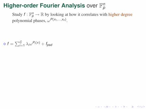
Higher-order Fourier Analysis over Fnp

Study f : Fnp → R by looking at how it correlates with higher degree

polynomial phases, ωP(x1,...,xn).

� f =∑C

i=1 λiωPi (x) + fpsd

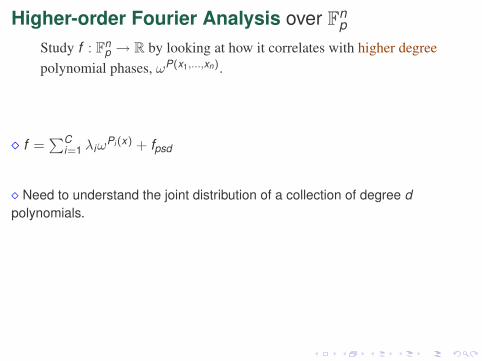
Higher-order Fourier Analysis over Fnp

Study f : Fnp → R by looking at how it correlates with higher degree

polynomial phases, ωP(x1,...,xn).

� f =∑C

i=1 λiωPi (x) + fpsd

� Need to understand the joint distribution of a collection of degree dpolynomials.

Higher-order Fourier Analysis over Fnp

Study f : Fnp → R by looking at how it correlates with higher degree

polynomial phases, ωP(x1,...,xn).

� f =∑C

i=1 λiωPi (x) + fpsd

Problem: P1, ...,PC ∈ P≤d (Fnp). X ,Y ∈ Fn

p uniform. Characterize thedistribution of

P1(X ) . . . P10(X )P1(X + Y ) . . . P10(X + Y )...P1(X + 4Y ) . . . P10(X + 4Y )

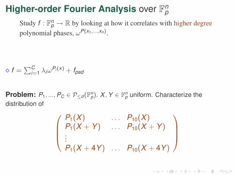
Higher-order Fourier Analysis over Fnp

Study f : Fnp → R by looking at how it correlates with higher degree

polynomial phases, ωP(x1,...,xn).

� f =∑C

i=1 λiωPi (x) + fpsd

Problem: P1, ...,PC ∈ P≤d (Fnp). X ,Y ∈ Fn

p uniform. Characterize thedistribution of

P1(X ) . . . P10(X )P1(X + Y ) . . . P10(X + Y )...P1(X + 4Y ) . . . P10(X + 4Y )

[HHL ‘15 (general case), BFHHL’13 (affine linear forms)]

[KL’08 and GT’09]: Distribution of (P1(X ), ...,PC(X )).

Problem 1. [KLP ’10, BL ’15]Number of degree d polynomials in Fp[x1, ..., xn] in hamming ballof radius δe − ε is 2O(nd−e).

Problem 2. [BHL ’15]Polynomial time algorithm for finding prescribed polynomial decompositions.

Problem 3. [BFL ’12, BFHHL ’13]Characterization of testable algebraic (i.e. affine invariant) properties.

Problem 1. [KLP ’10, BL ’15]Number of degree d polynomials in Fp[x1, ..., xn] in hamming ballof radius δe − ε is 2O(nd−e).

Problem 2. [BHL ’15]Polynomial time algorithm for finding prescribed polynomial decompositions.

Problem 3. [BFL ’12, BFHHL ’13]Characterization of testable algebraic (i.e. affine invariant) properties.

Problem 1. [KLP ’10, BL ’15]Number of degree d polynomials in Fp[x1, ..., xn] in hamming ballof radius δe − ε is 2O(nd−e).

Problem 2. [BHL ’15]Polynomial time algorithm for finding prescribed polynomial decompositions.

Problem 3. [BFL ’12, BFHHL ’13]Characterization of testable algebraic (i.e. affine invariant) properties.

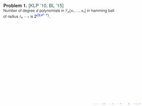
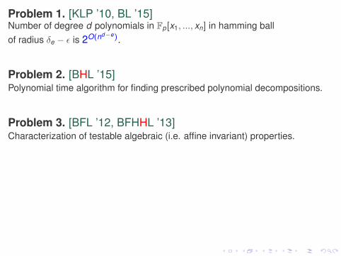
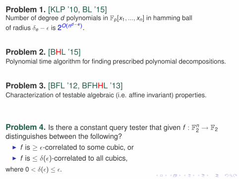
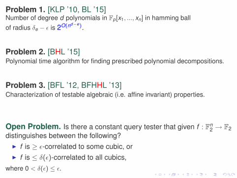
Problem 1. [KLP ’10, BL ’15]Number of degree d polynomials in Fp[x1, ..., xn] in hamming ballof radius δe − ε is 2O(nd−e).

Problem 2. [BHL ’15]Polynomial time algorithm for finding prescribed polynomial decompositions.

Problem 3. [BFL ’12, BFHHL ’13]Characterization of testable algebraic (i.e. affine invariant) properties.

Problem 4. Is there a constant query tester that given f : Fn2 → F2

distinguishes between the following?I f is ≥ ε-correlated to some cubic, orI f is ≤ δ(ε)-correlated to all cubics,

where 0 < δ(ε) ≤ ε.

Problem 1. [KLP ’10, BL ’15]Number of degree d polynomials in Fp[x1, ..., xn] in hamming ballof radius δe − ε is 2O(nd−e).

Problem 2. [BHL ’15]Polynomial time algorithm for finding prescribed polynomial decompositions.

Problem 3. [BFL ’12, BFHHL ’13]Characterization of testable algebraic (i.e. affine invariant) properties.

Open Problem. Is there a constant query tester that given f : Fn2 → F2

distinguishes between the following?I f is ≥ ε-correlated to some cubic, orI f is ≤ δ(ε)-correlated to all cubics,

where 0 < δ(ε) ≤ ε.

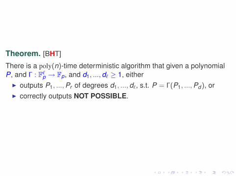
Theorem. [BHT]

There is a poly(n)-time deterministic algorithm that given a polynomialP, and Γ : F`p → Fp, and d1, ...,d` ≥ 1, either

I outputs P1, ...,Pr of degrees d1, ...,d`, s.t. P = Γ(P1, ...,Pd ), orI correctly outputs NOT POSSIBLE.

Proof illustration: Find P1,P2 of degree ≤ d − 1 such that

P = P1 · P2

. Algorithmic Regularity Lemma for Polynomials [BHT]:

P = Λ(Q1, ...,Qr )

. ∃xj s.t. for all i , deg(Qi) = deg(Qi |xj=0).

P|xj=0 = Λ(Q1|xj=0, ...,Qr |xj=0)

. Recurse on P|xj=0.I If NOT POSSIBLE, then output NOT POSSIBLE.I Otherwise we find P ′

1,P′2 such that P|xj=0 = P ′

1P ′2.

Proof illustration: Find P1,P2 of degree ≤ d − 1 such that

P = P1 · P2

. Algorithmic Regularity Lemma for Polynomials [BHT]:

P = Λ(Q1, ...,Qr )

. ∃xj s.t. for all i , deg(Qi) = deg(Qi |xj=0).

P|xj=0 = Λ(Q1|xj=0, ...,Qr |xj=0)

. Recurse on P|xj=0.I If NOT POSSIBLE, then output NOT POSSIBLE.I Otherwise we find P ′

1,P′2 such that P|xj=0 = P ′

1P ′2.

Proof illustration: Find P1,P2 of degree ≤ d − 1 such that

P = P1 · P2

. Algorithmic Regularity Lemma for Polynomials [BHT]:

P = Λ(Q1, ...,Qr )

. ∃xj s.t. for all i , deg(Qi) = deg(Qi |xj=0).

P|xj=0 = Λ(Q1|xj=0, ...,Qr |xj=0)

. Recurse on P|xj=0.I If NOT POSSIBLE, then output NOT POSSIBLE.I Otherwise we find P ′

1,P′2 such that P|xj=0 = P ′

1P ′2.

Proof illustration: Find P1,P2 of degree ≤ d − 1 such that

P = P1 · P2

. Algorithmic Regularity Lemma for Polynomials [BHT]:

P = Λ(Q1, ...,Qr )

. ∃xj s.t. for all i , deg(Qi) = deg(Qi |xj=0).

P|xj=0 = Λ(Q1|xj=0, ...,Qr |xj=0)

. Recurse on P|xj=0.I If NOT POSSIBLE, then output NOT POSSIBLE.I Otherwise we find P ′

1,P′2 such that P|xj=0 = P ′

1P ′2.

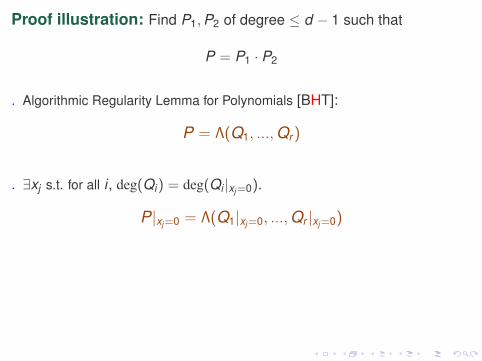
Proof illustration: Find P1,P2 of degree ≤ d − 1 such that

P = P1 · P2

. Algorithmic Regularity Lemma for Polynomials [BHT]:

P = Λ(Q1, ...,Qr )

. ∃xj s.t. for all i , deg(Qi) = deg(Qi |xj=0).

P|xj=0 = Λ(Q1|xj=0, ...,Qr |xj=0)

. Recurse on P|xj=0.I If NOT POSSIBLE, then output NOT POSSIBLE.I Otherwise we find P ′

1,P′2 such that P|xj=0 = P ′

1P ′2.

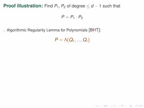
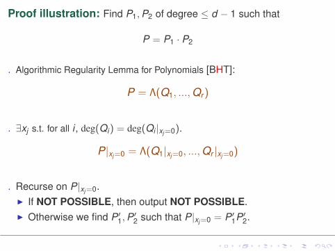
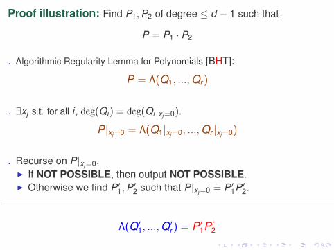
Λ(Q′1, ...,Q

′r ) = P ′

1P ′2

Proof illustration: Find P1,P2 of degree ≤ d − 1 such that

P = P1 · P2

. Algorithmic Regularity Lemma for Polynomials [BHT]:

P = Λ(Q1, ...,Qr )

. ∃xj s.t. for all i , deg(Qi) = deg(Qi |xj=0).

P|xj=0 = Λ(Q1|xj=0, ...,Qr |xj=0)

. Recurse on P|xj=0.I If NOT POSSIBLE, then output NOT POSSIBLE.I Otherwise we find P ′

1,P′2 such that P|xj=0 = P ′

1P ′2.

Λ(Q′1, ...,Q

′r ) = G1(Q′

1, ...,Q′r ,R1, ...,RC) ·G2(Q′

1, ...,Q′r ,R1, ...,RC)

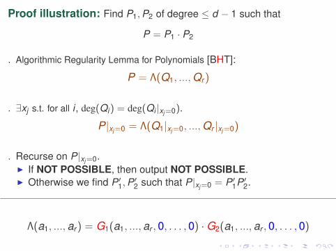
Proof illustration: Find P1,P2 of degree ≤ d − 1 such that

P = P1 · P2

. Algorithmic Regularity Lemma for Polynomials [BHT]:

P = Λ(Q1, ...,Qr )

. ∃xj s.t. for all i , deg(Qi) = deg(Qi |xj=0).

P|xj=0 = Λ(Q1|xj=0, ...,Qr |xj=0)

. Recurse on P|xj=0.I If NOT POSSIBLE, then output NOT POSSIBLE.I Otherwise we find P ′

1,P′2 such that P|xj=0 = P ′

1P ′2.

Λ(a1, ...,ar ) = G1(a1, ...,ar ,0, . . . ,0) ·G2(a1, ...,ar ,0, . . . ,0)

Proof illustration: Find P1,P2 of degree ≤ d − 1 such that

P = P1 · P2

. Algorithmic Regularity Lemma for Polynomials [BHT]:

P = Λ(Q1, ...,Qr )

. ∃xj s.t. for all i , deg(Qi) = deg(Qi |xj=0).

P|xj=0 = Λ(Q1|xj=0, ...,Qr |xj=0)

. Recurse on P|xj=0.I If NOT POSSIBLE, then output NOT POSSIBLE.I Otherwise we find P ′

1,P′2 such that P|xj=0 = P ′

1P ′2.

P = Λ(Q1, ...,Qr ) = G1(Q1, ...,Qr ,0, . . . ,0) ·G2(Q1, ...,Qr ,0, . . . ,0)

�