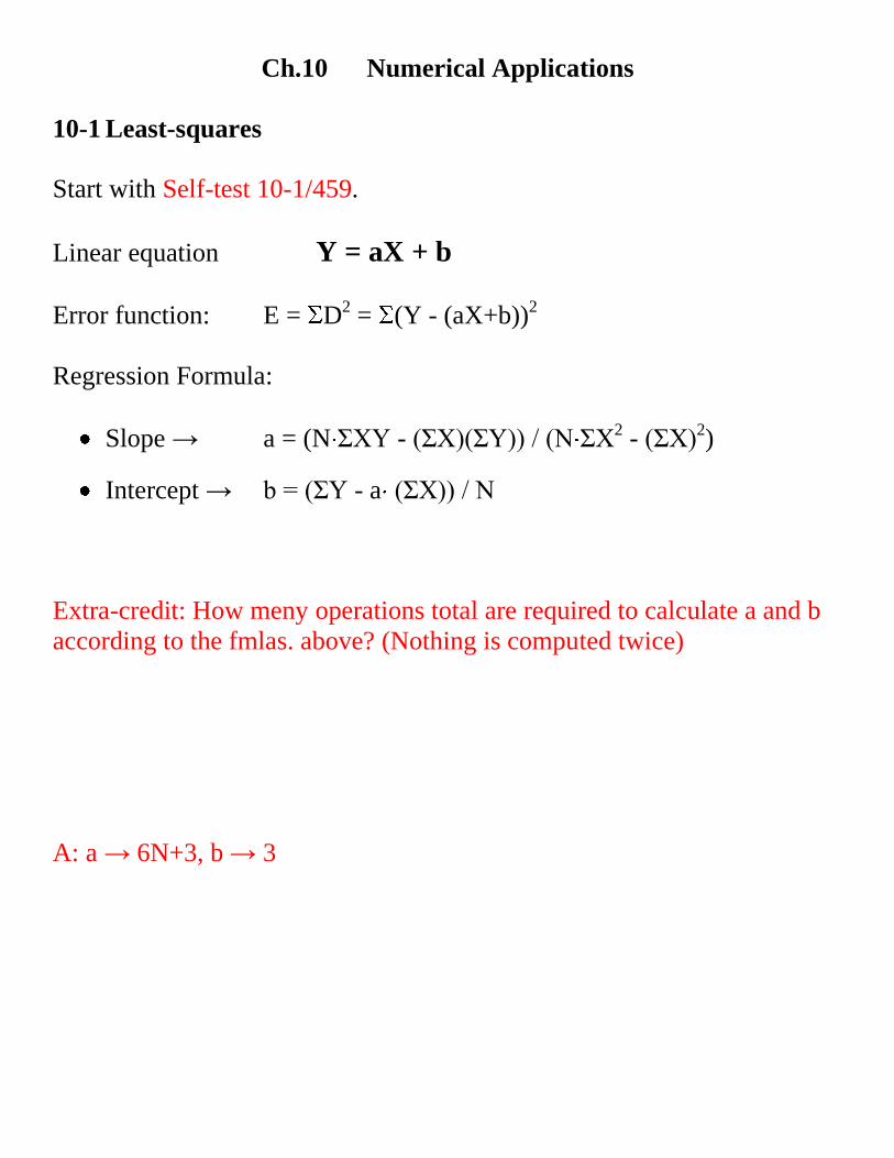
Ch.10 Numerical Applications

10-1 Least-squares

Start with Self-test 10-1/459.

Linear equation Y = aX + b

Error function: E = D2 = (Y - (aX+b))2

Regression Formula:

Slope → a = (N ΣXY - (ΣX)(ΣY)) / (N ΣX2 - (ΣX)2)

Intercept → b = (ΣY - a (ΣX)) / N

Extra-credit: How meny operations total are required to calculate a and b

according to the fmlas. above? (Nothing is computed twice)

A: a → 6N+3, b → 3

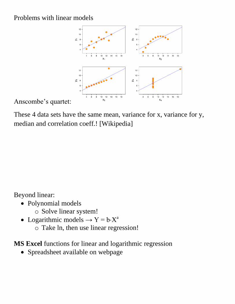
Problems with linear models

Anscombe’s quartet:

These 4 data sets have the same mean, variance for x, variance for y,

median and correlation coeff.! [Wikipedia]

Beyond linear:

Polynomial models

o Solve linear system!

Logarithmic models → Y = b Xa

o Take ln, then use linear regression!

MS Excel functions for linear and logarithmic regression

Spreadsheet available on webpage

10-3 Matrix Operations

Scalar multiplication

Matrix add., sub.

Dot product (vector mult.)

Matrix mult.

Self-test 10-2 / 472

------------------------------------------------------------------------------

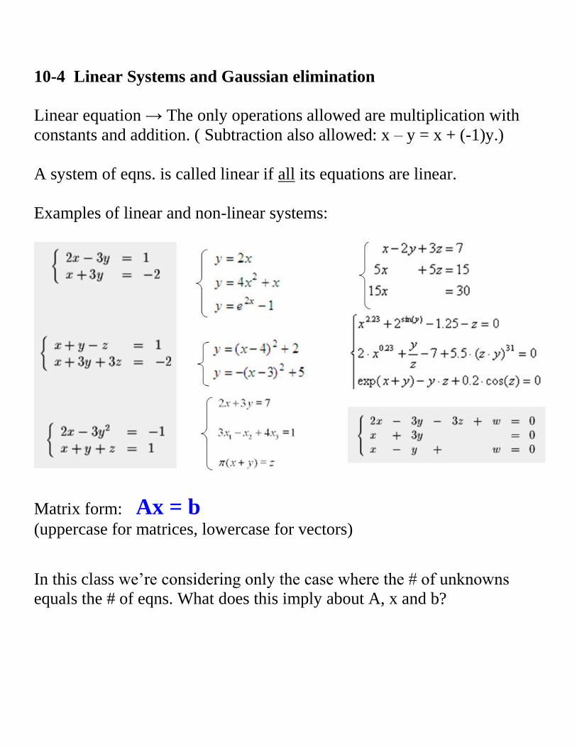
10-4 Linear Systems and Gaussian elimination

Linear equation → The only operations allowed are multiplication with

constants and addition. ( Subtraction also allowed: x – y = x + (-1)y.)

A system of eqns. is called linear if all its equations are linear.

Examples of linear and non-linear systems:

Matrix form: Ax = b

(uppercase for matrices, lowercase for vectors)

In this class we’re considering only the case where the # of unknowns

equals the # of eqns. What does this imply about A, x and b?

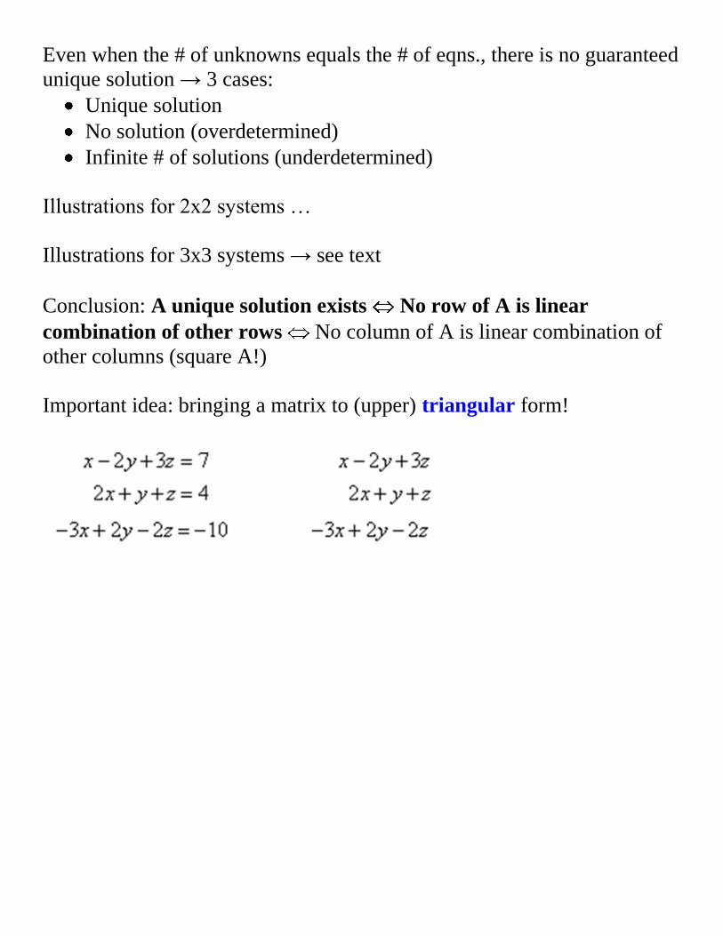
Even when the # of unknowns equals the # of eqns., there is no guaranteed

unique solution → 3 cases:

Unique solution

No solution (overdetermined)

Infinite # of solutions (underdetermined)

Illustrations for 2x2 systems …

Illustrations for 3x3 systems → see text

Conclusion: A unique solution exists No row of A is linear

combination of other rows No column of A is linear combination of

other columns (square A!)

Important idea: bringing a matrix to (upper) triangular form!

Handout: Bring this matrix to upper triangular form:

----------------------------------------------------------------------------------

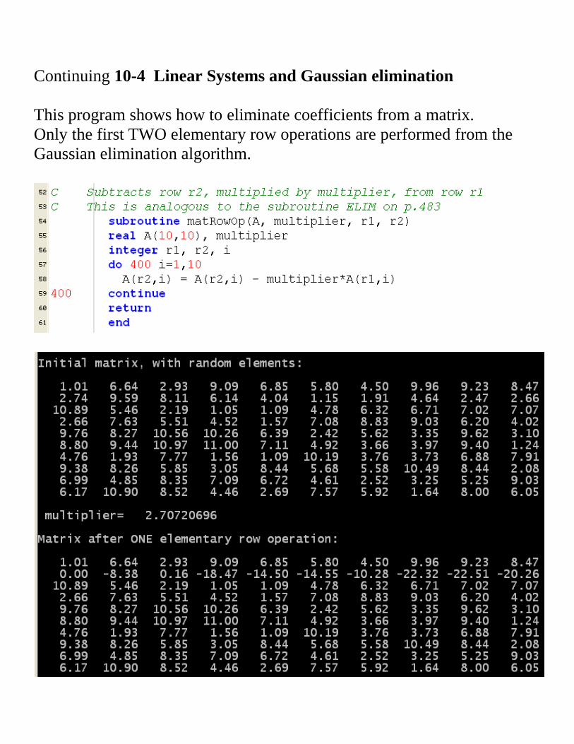
Continuing 10-4 Linear Systems and Gaussian elimination

This program shows how to eliminate coefficients from a matrix.

Only the first TWO elementary row operations are performed from the

Gaussian elimination algorithm.

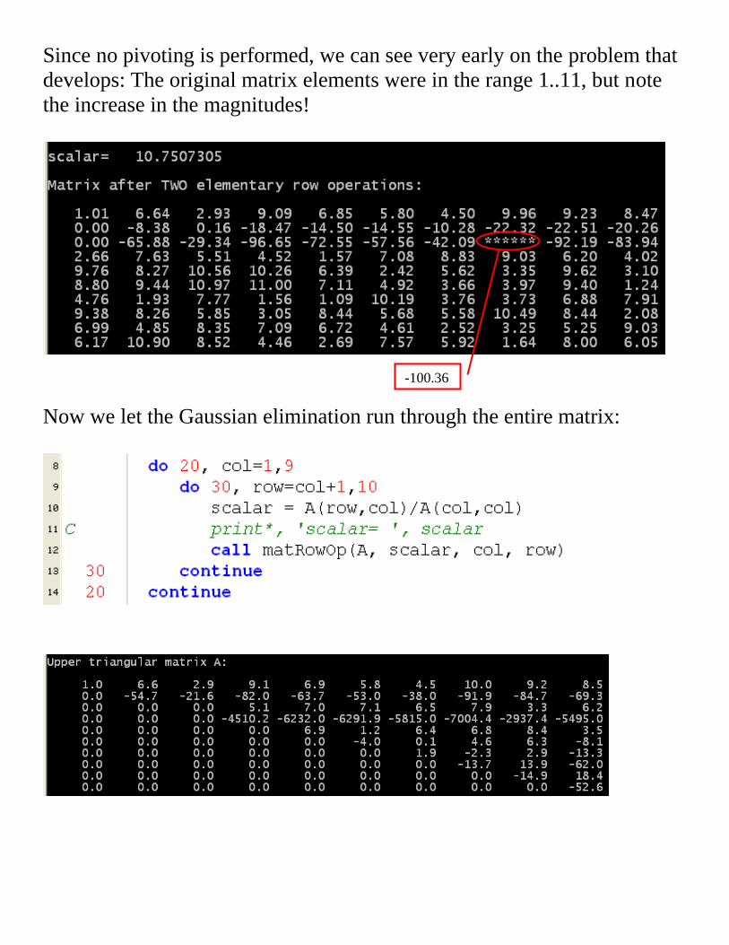
Since no pivoting is performed, we can see very early on the problem that

develops: The original matrix elements were in the range 1..11, but note

the increase in the magnitudes!

Now we let the Gaussian elimination run through the entire matrix:

-100.36

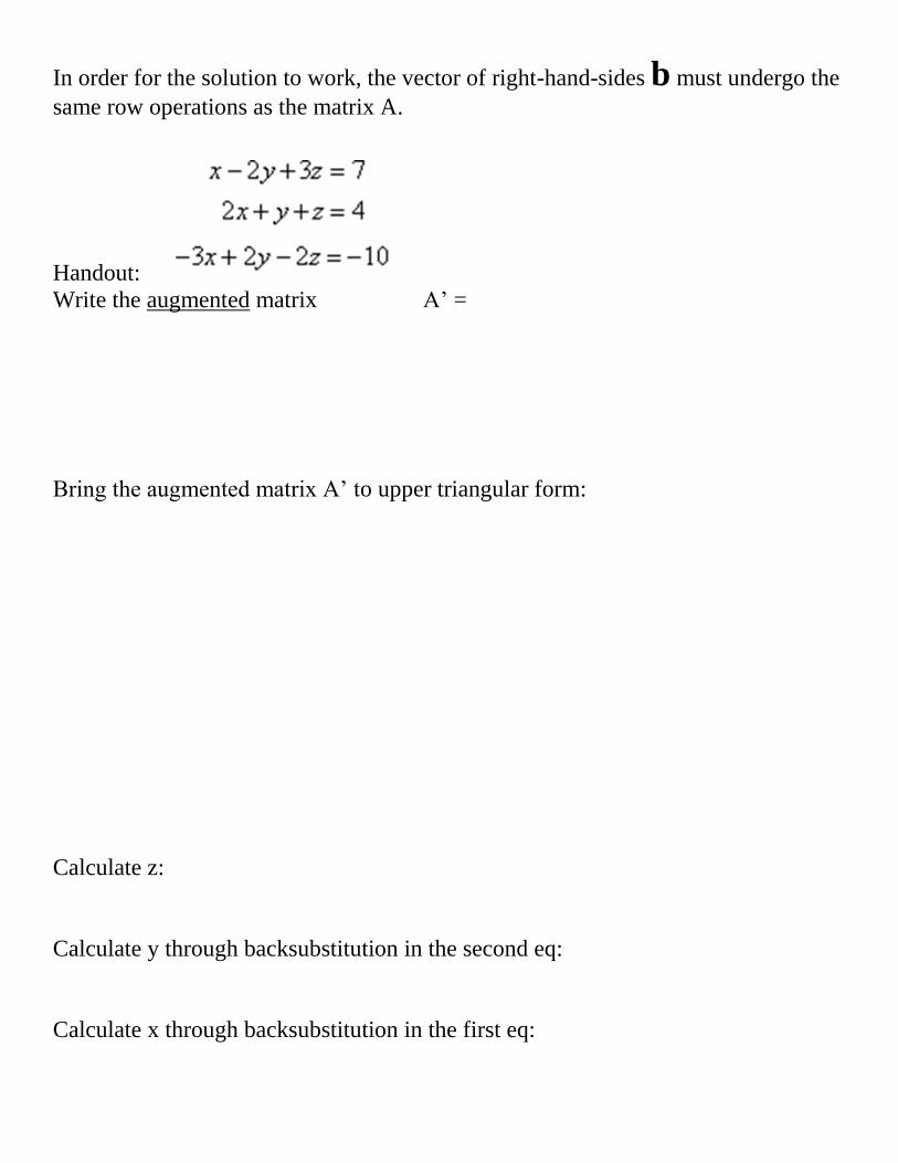
In order for the solution to work, the vector of right-hand-sides b must undergo the

same row operations as the matrix A.

Handout: Write the augmented matrix A’ =

Bring the augmented matrix A’ to upper triangular form:

Calculate z:

Calculate y through backsubstitution in the second eq:

Calculate x through backsubstitution in the first eq:

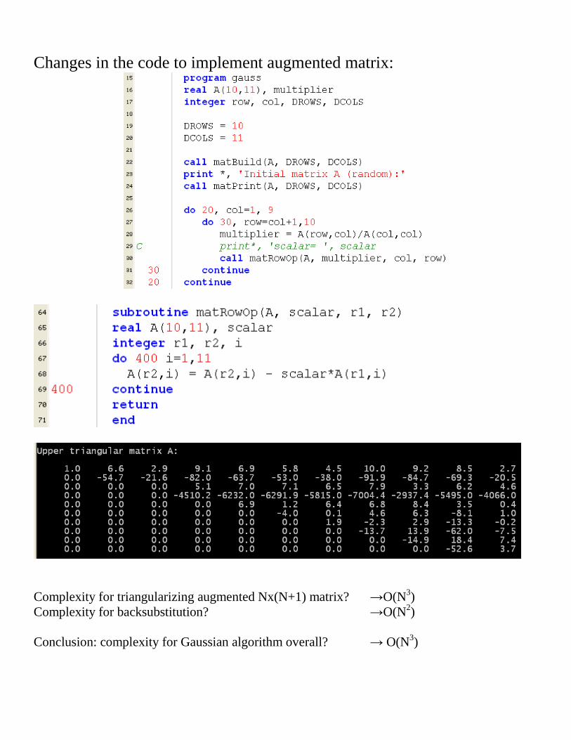
Changes in the code to implement augmented matrix:

Complexity for triangularizing augmented Nx(N+1) matrix? →O(N3)

Complexity for backsubstitution? →O(N2)

Conclusion: complexity for Gaussian algorithm overall? → O(N3)

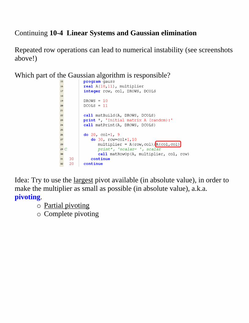
Continuing 10-4 Linear Systems and Gaussian elimination

Repeated row operations can lead to numerical instability (see screenshots

above!)

Which part of the Gaussian algorithm is responsible?

Idea: Try to use the largest pivot available (in absolute value), in order to

make the multiplier as small as possible (in absolute value), a.k.a.

pivoting.

o Partial pivoting

o Complete pivoting

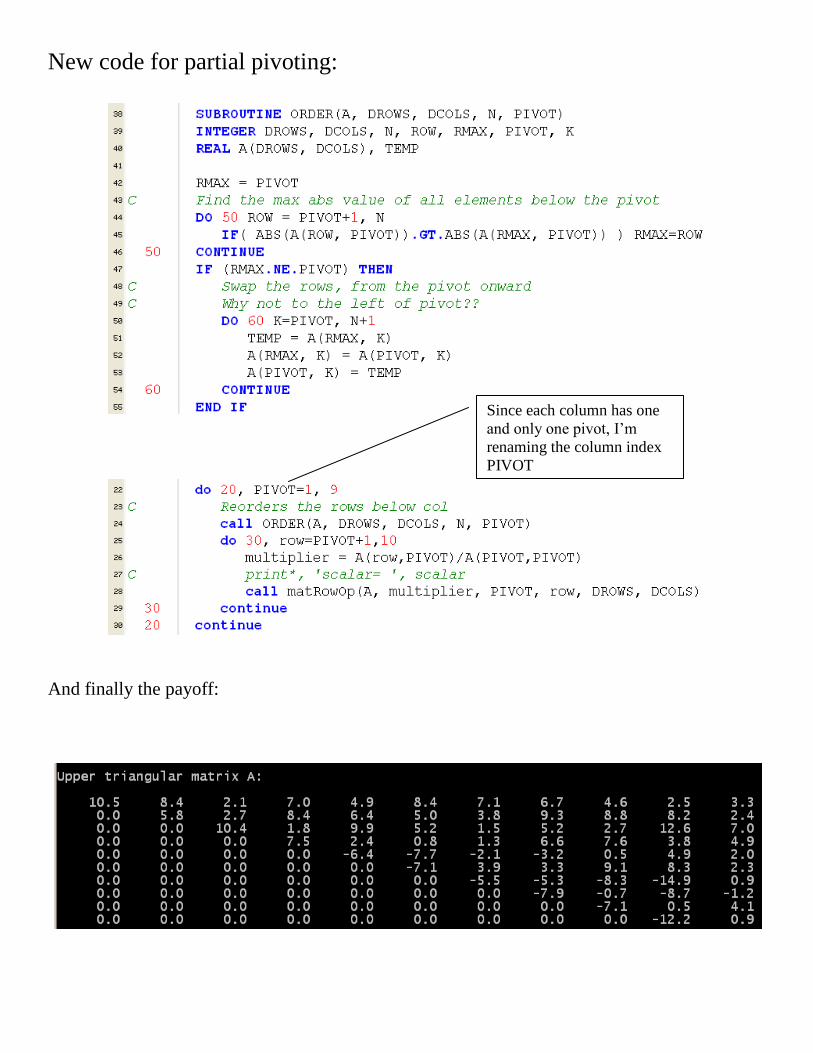
New code for partial pivoting:

And finally the payoff:

Since each column has one

and only one pivot, I’m

renaming the column index

PIVOT

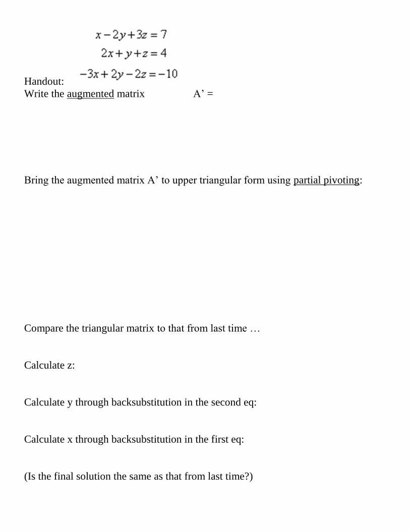
Handout: Write the augmented matrix A’ =

Bring the augmented matrix A’ to upper triangular form using partial pivoting:

Compare the triangular matrix to that from last time …

Calculate z:

Calculate y through backsubstitution in the second eq:

Calculate x through backsubstitution in the first eq:

(Is the final solution the same as that from last time?)

Individual work for next time: Solve in notebook the Hand Example on

pp.479-480.

How about total pivoting? … Swapping columns can lead to an even larger pivot, but the price

to pay is that the unknowns get swapped, too. We have to keep track of these swaps, and un-

swap the solution vector at the end.

Empirical conclusion: partial pivoting is good enough in most practical problems. If the matrix

A is particularly ill-conditioned, we can work a little harder and do complete pivoting.

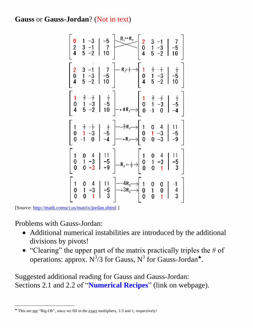
Gauss or Gauss-Jordan? (Not in text)

[Source: http://math.comsci.us/matrix/jordan.shtml ]

Problems with Gauss-Jordan:

Additional numerical instabilities are introduced by the additional

divisions by pivots!

“Clearing” the upper part of the matrix practically triples the # of

operations: approx. N3/3 for Gauss, N3 for Gauss-Jordan .

Suggested additional reading for Gauss and Gauss-Jordan:

Sections 2.1 and 2.2 of “Numerical Recipes” (link on webpage).

This are not “Big-Oh”, since we fill in the exact multipliers, 1/3 and 1, respectively!

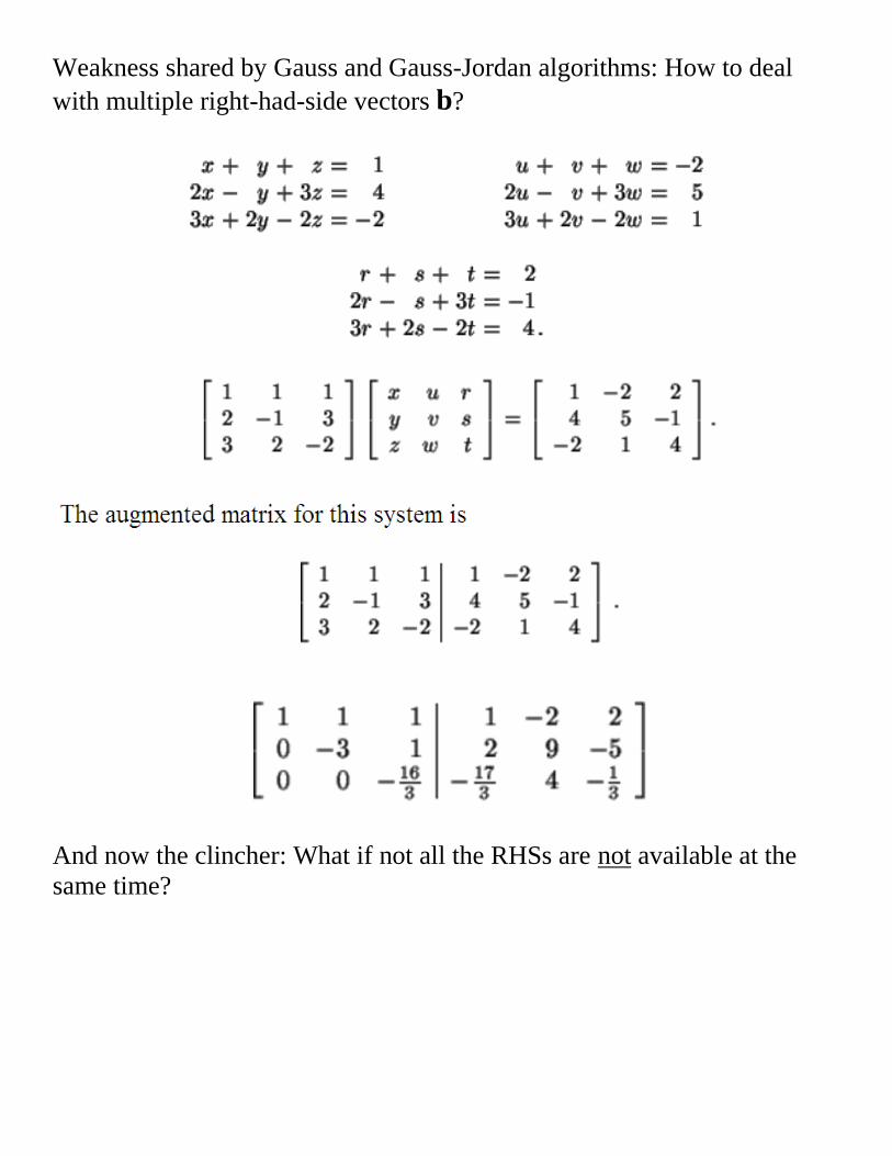
Weakness shared by Gauss and Gauss-Jordan algorithms: How to deal

with multiple right-had-side vectors b?

And now the clincher: What if not all the RHSs are not available at the

same time?

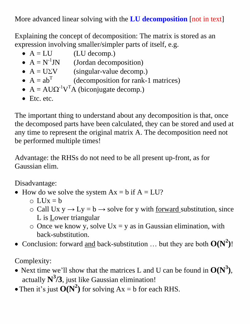
More advanced linear solving with the LU decomposition [not in text]

Explaining the concept of decomposition: The matrix is stored as an

expression involving smaller/simpler parts of itself, e.g.

A = LU (LU decomp.)

A = N-1JN (Jordan decomposition)

A = U V (singular-value decomp.)

A = abT (decomposition for rank-1 matrices)

A = AU -1VTA (biconjugate decomp.)

Etc. etc.

The important thing to understand about any decomposition is that, once

the decomposed parts have been calculated, they can be stored and used at

any time to represent the original matrix A. The decomposition need not

be performed multiple times!

Advantage: the RHSs do not need to be all present up-front, as for

Gaussian elim.

Disadvantage:

How do we solve the system Ax = b if A = LU?

o LUx = b

o Call Ux y → Ly = b → solve for y with forward substitution, since

L is Lower triangular

o Once we know y, solve Ux = y as in Gaussian elimination, with

back-substitution.

Conclusion: forward and back-substitution … but they are both O(N2)!

Complexity:

Next time we’ll show that the matrices L and U can be found in O(N3),

actually N3/3, just like Gaussian elimination!

Then it’s just O(N2) for solving Ax = b for each RHS.

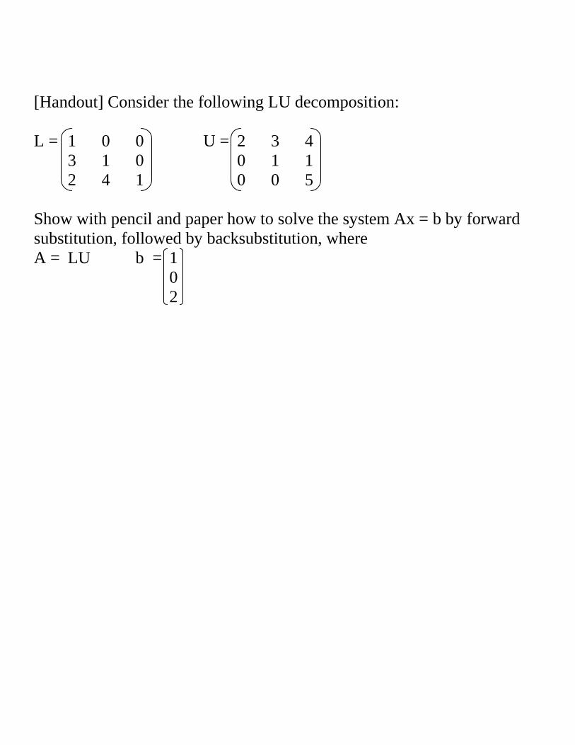
[Handout] Consider the following LU decomposition:

L = 1 0 0 U = 2 3 4

3 1 0 0 1 1

2 4 1 0 0 5

Show with pencil and paper how to solve the system Ax = b by forward

substitution, followed by backsubstitution, where

A = LU b = 1

0

2

A note on L’s diagonal:

L and U together have N2 + N non-zero elements. Because the original A

has only N2, we can choose the remaining N freely. Most implementations

of LU decomp. choose to make all diag. elements of L ones. In this case,

we don’t even need two matrices, we can store both L and U in place in

the old matrix A!

Recommended reading:

Section 2.3 of Numerical Recipes (link on webpage)

Wikipedia article (link on webpage)

------------------------------------------------------------------------------