Efficient matrix multiplication

J.M. Landsberg

Texas A&M University

ILAS July 2019Supported by NSF grant CCF-1814254

1 / 25

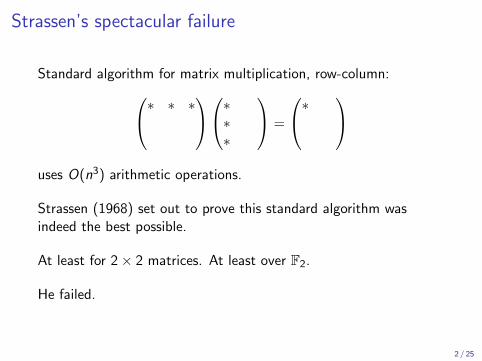
Strassen’s spectacular failure

Standard algorithm for matrix multiplication, row-column:∗ ∗ ∗∗∗∗

=

∗ uses O(n3) arithmetic operations.

Strassen (1968) set out to prove this standard algorithm wasindeed the best possible.

At least for 2× 2 matrices. At least over F2.

He failed.

2 / 25

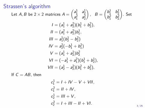
Strassen’s algorithm

Let A,B be 2× 2 matrices A =

(a11 a12a21 a22

), B =

(b11 b12b21 b22

). Set

I = (a11 + a22)(b11 + b22),

II = (a21 + a22)b11,

III = a11(b12 − b22)

IV = a22(−b11 + b21)

V = (a11 + a12)b22

VI = (−a11 + a21)(b11 + b12),

VII = (a12 − a22)(b21 + b22),

If C = AB, then

c11 = I + IV − V + VII ,

c21 = II + IV ,

c12 = III + V ,

c22 = I + III − II + VI .3 / 25

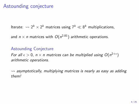
Astounding conjecture

Iterate: 2k × 2k matrices using 7k � 8k multiplications,

and n × n matrices with O(n2.81) arithmetic operations.

Astounding Conjecture

For all ε > 0, n × n matrices can be multiplied using O(n2+ε)arithmetic operations.

asymptotically, multiplying matrices is nearly as easy as addingthem!

4 / 25

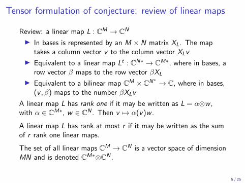
Tensor formulation of conjecture: review of linear maps

Review: a linear map L : CM → CN

I In bases is represented by an M × N matrix XL. The maptakes a column vector v to the column vector XLv

I Equivalent to a linear map Lt : CN∗ → CM∗, where in bases, arow vector β maps to the row vector βXL

I Equivalent to a bilinear map CM × CN∗ → C, where in bases,(v , β) maps to the number βXLv

A linear map L has rank one if it may be written as L = α⊗w ,with α ∈ CM∗, w ∈ CN . Then v 7→ α(v)w .

A linear map L has rank at most r if it may be written as the sumof r rank one linear maps.

The set of all linear maps CM → CN is a vector space of dimensionMN and is denoted CM∗⊗CN .

5 / 25

Tensor formulation of conjecture

Set N = n2.Matrix multiplication is a bilinear map

M〈n〉 : CN × CN → CN ,

i.e., an element ofCN∗⊗CN∗⊗CN

Bilinear maps CN × CN → CN may also be viewed as trilinearmaps CN × CN × CN∗ → C.Exercise: As such, M〈n〉(X ,Y ,Z ) = trace(XYZ ).

6 / 25

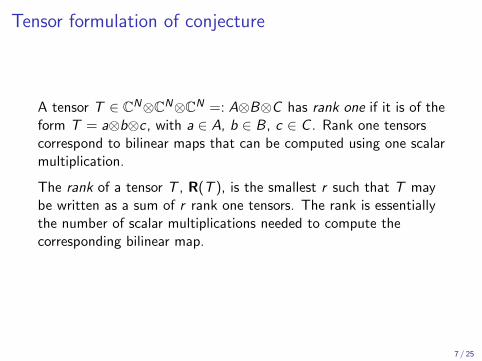
Tensor formulation of conjecture

A tensor T ∈ CN⊗CN⊗CN =: A⊗B⊗C has rank one if it is of theform T = a⊗b⊗c , with a ∈ A, b ∈ B, c ∈ C . Rank one tensorscorrespond to bilinear maps that can be computed using one scalarmultiplication.

The rank of a tensor T , R(T ), is the smallest r such that T maybe written as a sum of r rank one tensors. The rank is essentiallythe number of scalar multiplications needed to compute thecorresponding bilinear map.

7 / 25

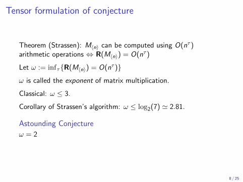
Tensor formulation of conjecture

Theorem (Strassen): M〈n〉 can be computed using O(nτ )arithmetic operations ⇔ R(M〈n〉) = O(nτ )

Let ω := infτ{R(M〈n〉) = O(nτ )}

ω is called the exponent of matrix multiplication.

Classical: ω ≤ 3.

Corollary of Strassen’s algorithm: ω ≤ log2(7) ' 2.81.

Astounding Conjecture

ω = 2

8 / 25

Geometric formulation of conjecture

Imagine this curve represents the set of tensors of rank one.

9 / 25

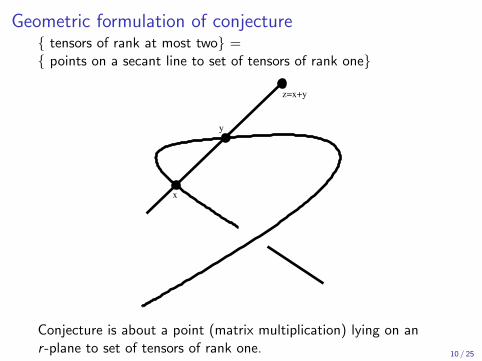
Geometric formulation of conjecture{ tensors of rank at most two} ={ points on a secant line to set of tensors of rank one}

x

y

z=x+y

Conjecture is about a point (matrix multiplication) lying on anr -plane to set of tensors of rank one. 10 / 25

Bini’s sleepless nights

Bini-Capovani-Lotti-Romani (1979) investigated if M〈2〉, with onematrix entry set to zero, could be computed with fivemultiplications (instead of the naıve 6), i.e., if this reduced matrixmultiplication tensor had rank 5.

They used numerical methods.

Their code appeared to have a problem.

11 / 25

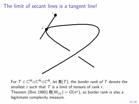
The limit of secant lines is a tangent line!

u

v

For T ∈ CN⊗CN⊗CN , let R(T ), the border rank of T denote thesmallest r such that T is a limit of tensors of rank r .Theorem (Bini 1980) R(M〈n〉) = O(nω), so border rank is also alegitimate complexity measure.

12 / 25

Wider geometric perspective

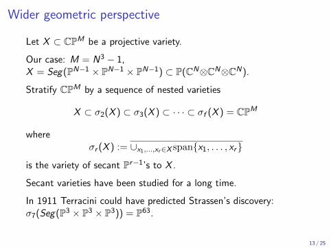
Let X ⊂ CPM be a projective variety.

Our case: M = N3 − 1,X = Seg(PN−1 × PN−1 × PN−1) ⊂ P(CN⊗CN⊗CN).

Stratify CPM by a sequence of nested varieties

X ⊂ σ2(X ) ⊂ σ3(X ) ⊂ · · · ⊂ σf (X ) = CPM

whereσr (X ) := ∪x1,...,xr∈X span{x1, . . . , xr}

is the variety of secant Pr−1’s to X .

Secant varieties have been studied for a long time.

In 1911 Terracini could have predicted Strassen’s discovery:σ7(Seg(P3 × P3 × P3)) = P63.

13 / 25

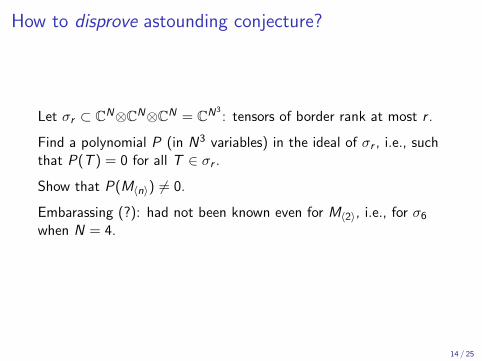
How to disprove astounding conjecture?

Let σr ⊂ CN⊗CN⊗CN = CN3: tensors of border rank at most r .

Find a polynomial P (in N3 variables) in the ideal of σr , i.e., suchthat P(T ) = 0 for all T ∈ σr .

Show that P(M〈n〉) 6= 0.

Embarassing (?): had not been known even for M〈2〉, i.e., for σ6when N = 4.

14 / 25

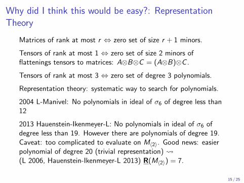
Why did I think this would be easy?: RepresentationTheory

Matrices of rank at most r ⇔ zero set of size r + 1 minors.

Tensors of rank at most 1 ⇔ zero set of size 2 minors offlattenings tensors to matrices: A⊗B⊗C = (A⊗B)⊗C .

Tensors of rank at most 3 ⇔ zero set of degree 3 polynomials.

Representation theory: systematic way to search for polynomials.

2004 L-Manivel: No polynomials in ideal of σ6 of degree less than12

2013 Hauenstein-Ikenmeyer-L: No polynomials in ideal of σ6 ofdegree less than 19. However there are polynomials of degree 19.Caveat: too complicated to evaluate on M〈2〉. Good news: easierpolynomial of degree 20 (trivial representation) (L 2006, Hauenstein-Ikenmeyer-L 2013) R(M〈2〉) = 7.

15 / 25

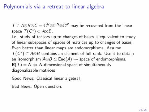
Polynomials via a retreat to linear algebra

T ∈ A⊗B⊗C = CN⊗CN⊗CN may be recovered from the linearspace T (C ∗) ⊂ A⊗B.I.e., study of tensors up to changes of bases is equivalent to studyof linear subspaces of spaces of matrices up to changes of bases.Even better than linear maps are endomorphisms. AssumeT (C ∗) ⊂ A⊗B contains an element of full rank. Use it to obtainan isomorphism A⊗B ' End(A) space of endomorphisms.R(T ) = N ⇔ N-dimensional space of simultaneouslydiagonalizable matrices

Good News: Classical linear algebra!

Bad News: Open question.

16 / 25

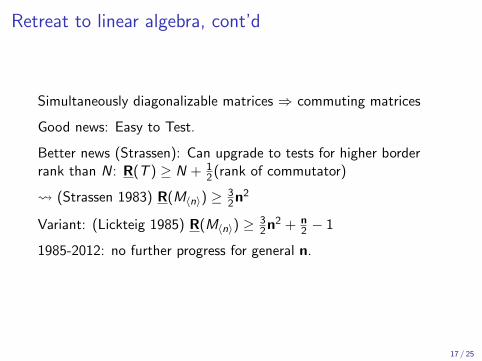
Retreat to linear algebra, cont’d

Simultaneously diagonalizable matrices ⇒ commuting matrices

Good news: Easy to Test.

Better news (Strassen): Can upgrade to tests for higher borderrank than N: R(T ) ≥ N + 1

2(rank of commutator)

(Strassen 1983) R(M〈n〉) ≥ 32n

2

Variant: (Lickteig 1985) R(M〈n〉) ≥ 32n

2 + n2 − 1

1985-2012: no further progress for general n.

17 / 25

Retreat to linear algebra, cont’d

Perspective: Strassen mapped space of tensors to space ofmatrices, found equations by taking minors.

Classical trick in algebraic geometry to find equations via minors. (L-Ottaviani 2013) R(M〈n〉) ≥ 2n2 − n

For those familiar with representation theory: found via aG = GL(A)× GL(B)× GL(C ) module map to a space of matrices(systematic search possible).

Punch line: Found equations by exploiting symmetry of σr

18 / 25

Bad News: Barriers

Theorem (Bernardi-Ranestad,Buczynski-Galcazka,Efremenko-Garg-Oliviera-Wigderson): Game (almost) over for determinantalmethods.

For the experts: Variety of zero dimensional schemes of length r isnot irreducible r > 13. Determinantal methods detect zerodimensional schemes (want zero dimensional smoothable schemes).

19 / 25

How to go further?

So far, lower bounds via symmetry of σr .

The matrix multiplication tensor also has symmetry:

T ∈ CN⊗CN⊗CN , define symmetry group of TGT := {g ∈ GL×3N | g · T = T}

GL×3n ⊂ GM〈n〉 ⊂ GL×3n2

:

For (g1, g2, g3) ∈ GL×3n

trace(XYZ ) = trace((g1Xg2−1)(g2Yg3

−1)(g3Zg1−1)

20 / 25

How to exploit GT?

Given T ∈ A⊗B⊗CR(T ) ≤ r ⇔ ∃ curve Et ⊂ G (r ,A⊗B⊗C ) such thati) For t 6= 0, Et is spanned by r rank one elements.ii) T ∈ E0.

For all g ∈ GT , gEt also works. can insist on normalized curves (for M〈n〉, those with E0 Borelstable).

(L-Michalek 2017) R(M〈n〉) ≥ 2n2 − log2n− 1

More bad news: this method cannot go much further.

21 / 25

Upper bounds: How to prove conjecture?

History: M〈n〉 too complicated, look for something simpler.Schonhage:

R(M〈1,(n−1)2,(n−1)2〉 ⊕M〈n,n,1〉) = n2 + 1

<< R(M〈1,(n−1)2,(n−1)2〉) + R(M〈n,n,1〉)

Can upper bound ω by upper bounding border ranks of such sums.Showed ω < 2.55

22 / 25

Upper bounds

T ∈ A⊗B⊗C , define Kronecker powerT�k ∈ (A⊗k)⊗(B⊗k)⊗(C⊗k).

Exercise: M�k〈n〉 = M〈nk 〉 (self-reproducing property!)

Strassen: Look for “simple” T such that T�k degenerates todirect sum of many disjoint rectangular matrix multiplications. ω < 2.38 (Strassen, Coppersmith-Winograd 1989) via “bigCoppersmith-Winograd tensor”

1989-2011 no improvment2011-2013 ω < 2.373 (Stouthers-Williams-LeGall)2014 Bad news: Ambainus-Filimus-LeGall: game over for bigCoppersmith-Winograd tensor — need new tensors!

2019: Conner-Gesmundo-L-Ventura: New tensors, potentiallybetter for Strassen’s method — stay tuned.

23 / 25

New idea, following Buczynska-Buczynski: Upper andLower bounds

Use more algebraic geometry: Consider not just curve of r points,but the curve of ideals it gives rise to: border apolarity method

Can insist that limiting ideal is Borel fixed: reduces to small search.

Conner-Harper-L May 2019: very easy algebraic proof R(M〈2〉) = 7

Recall: Strassen R(M〈3〉) ≥ 14, L-Ottaviani R(M〈3〉) ≥ 15,L-Michalek R(M〈3〉) ≥ 16.

Conner-Harper-L June 2019: R(M〈3〉) ≥ 17 (so far - work inprogress).

Bonus 1: Method in principle can overcome lower bound barriers.

Bonus 2: Method also can be used for upper bounds.

24 / 25

Thank you for your attention

For more on tensors, their geometry and applications, resp.geometry and complexity, resp. recent developments:

25 / 25