1

Users’ guide to FAC-PACK

A software for the computation

of multi-component factorizations

and the area of feasible solutions

Software version 1.0

Mathias Sawalla and Klaus Neymeyra,b

a Institut für Mathematik,Universität Rostock, Ulmenstrasse 69, 18057 Rostock.

b Leibniz-Institut für Katalyse, Albert-Einstein-Strasse 60, 18069 Rostock.

Email: α =mathias.sawall and β =klaus.neymeyr with {α or β}@uni-rostock.de

May 23, 2013

FAC-PACK is a software for the computation of nonnegative multi-compo-nent factorizations and for the numerical approximation of the area of feasiblesolutions (AFS). FAC-PACK comes with a graphical user interface (GUI) inMatLab. The GUI provides the functionality for computing a low rankapproximation of the data matrix, for determining an initial nonnegativematrix factorization, for approximating the AFS by the polygon inflationmethod, as well as for graphically representing the admissible spectral andconcentration factors. Currently, FAC-PACK can be applied to two- andthree-component systems.

A special feature of the AFS representation is its live-view mode whichallows an interactive visual inspection of the spectra or concentration profileswhile moving the mouse pointer through the AFS. For two-component sys-tems the full solution is presented in the live-view mode. For three-componentsystems the GUI provides a further functionality: If a certain point of theAFS is locked (i.e. some known spectrum has been detected or some additionalinformation on the system has been used), then the associated reduced andsmaller AFS can be computed. This locking-and-AFS-reduction procedurecan be repeated.

The FAC-PACK GUI has been implemented on MatLab. No additionalpackages or MatLab-toolboxes are needed. The computational core of FAC-PACK is written in C which includes an implementation of the polygon in-flation procedure.

Contents 2

Contents

1 Quick reference 3

2 Quick start - for the impatient user 4

3 Introduction to FAC-PACK 6

4 Get ready to start 8

4.1 Program structure . . . . . . . . . . . . . . . . . . . . . . . . . . . . . . . 84.2 External C-routine . . . . . . . . . . . . . . . . . . . . . . . . . . . . . . . 94.3 Further included libraries . . . . . . . . . . . . . . . . . . . . . . . . . . . 9

5 Warming-up: Initial steps 10

5.1 Load problem data . . . . . . . . . . . . . . . . . . . . . . . . . . . . . . . 105.1.1 Test data . . . . . . . . . . . . . . . . . . . . . . . . . . . . . . . . 10

5.2 Transposing the problem . . . . . . . . . . . . . . . . . . . . . . . . . . . . 105.3 Initial NMF . . . . . . . . . . . . . . . . . . . . . . . . . . . . . . . . . . . 11

6 Computation of the AFS 13

6.1 Control parameters . . . . . . . . . . . . . . . . . . . . . . . . . . . . . . . 136.2 Type of polygon inflation . . . . . . . . . . . . . . . . . . . . . . . . . . . 14

7 Factor representation & live-view mode 16

7.1 Two-component systems . . . . . . . . . . . . . . . . . . . . . . . . . . . . 167.2 Three component systems . . . . . . . . . . . . . . . . . . . . . . . . . . . 16

8 Reduction of the rotational ambiguity 18

8.1 Locking a first spectrum . . . . . . . . . . . . . . . . . . . . . . . . . . . . 188.2 Locking a second spectrum . . . . . . . . . . . . . . . . . . . . . . . . . . 18

9 Appendix 20

9.1 Save data and extract axes . . . . . . . . . . . . . . . . . . . . . . . . . . . 209.2 Cancellation of the program . . . . . . . . . . . . . . . . . . . . . . . . . . 209.3 How to get help . . . . . . . . . . . . . . . . . . . . . . . . . . . . . . . . . 20

1. Quick reference 3

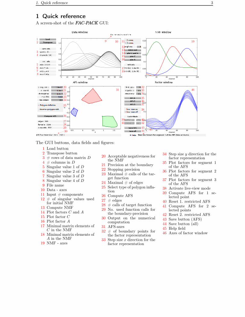
1 Quick referenceA screen-shot of the FAC-PACK GUI:

0 10 20 30 40 50 60 70 80 90 1000

0.2

0.4

0.6

0.8

1

1.2

channel0 20 40 60 80 100

0

0.05

0.1

0.15

0.2

0.25

channel

0 20 40 60 80 1000

0.05

0.1

0.15

0.2

channel−0.5 0 0.5 1 1.5

−0.8

−0.6

−0.4

−0.2

0

0.2

0.4

0.6

0.8

1

α

β

12

34

5678

9 10 11

1213141516

1718

19

2021222324

25

26

27282930

31323334

353637

38

39 4041 42

4344 45

46

The GUI buttons, data fields and figures:

1 Load button2 Transpose button3 # rows of data matrix D

4 # columns in D5 Singular value 1 of D6 Singular value 2 of D7 Singular value 3 of D8 Singular value 4 of D9 File name

10 Data - axes11 Input # components12 # of singular values used

for initial NMF13 Compute NMF14 Plot factors C and A

15 Plot factor C16 Plot factor A

17 Minimal matrix elements ofC in the NMF

18 Minimal matrix elements ofA in the NMF

19 NMF - axes

20 Acceptable negativeness forthe NMF

21 Precision at the boundary22 Stopping precision23 Maximal # calls of the tar-

get function24 Maximal # of edges25 Select type of polygon infla-

tion26 Compute AFS27 # edges28 # calls of target function29 No. used function calls for

the boundary-precision30 Output on the numerical

computation31 AFS-axes32 # of boundary points for

the factor representation33 Step size x direction for the

factor representation

34 Step size y direction for thefactor representation

35 Plot factors for segment 1of the AFS

36 Plot factors for segment 2of the AFS

37 Plot factors for segment 3of the AFS

38 Activate live-view mode39 Compute AFS for 1 se-

lected point40 Reset 1. restricted AFS41 Compute AFS for 2 se-

lected points42 Reset 2. restricted AFS43 Save button (AFS)44 Save button (all)45 Help field46 Axes of factor window

2. Quick start - for the impatient user 4

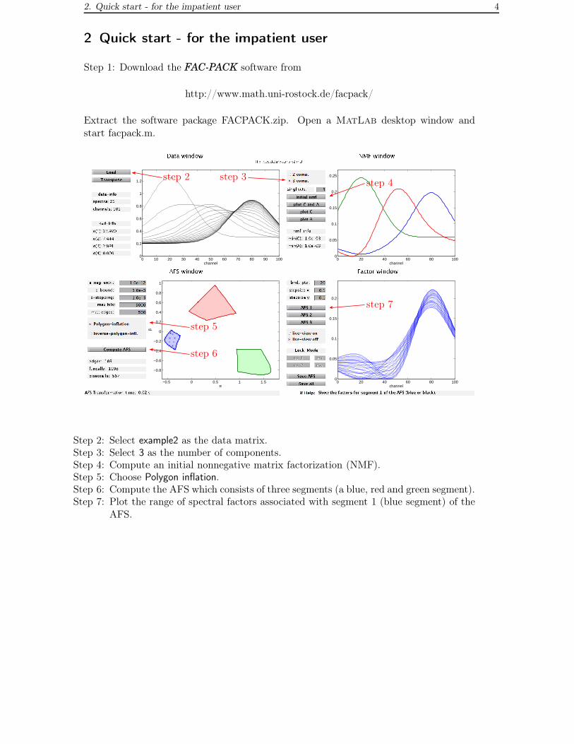
2 Quick start - for the impatient user

Step 1: Download the FAC-PACK software from

http://www.math.uni-rostock.de/facpack/

Extract the software package FACPACK.zip. Open a MatLab desktop window andstart facpack.m.

0 10 20 30 40 50 60 70 80 90 1000

0.2

0.4

0.6

0.8

1

1.2

channel0 20 40 60 80 100

0

0.05

0.1

0.15

0.2

0.25

channel

0 20 40 60 80 1000

0.05

0.1

0.15

0.2

channel−0.5 0 0.5 1 1.5

−0.8

−0.6

−0.4

−0.2

0

0.2

0.4

0.6

0.8

1

α

β

step 2 step 3step 4

step 5

step 6

step 7

Step 2: Select example2 as the data matrix.Step 3: Select 3 as the number of components.Step 4: Compute an initial nonnegative matrix factorization (NMF).Step 5: Choose Polygon inflation.Step 6: Compute the AFS which consists of three segments (a blue, red and green segment).Step 7: Plot the range of spectral factors associated with segment 1 (blue segment) of the

AFS.

2. Quick start - for the impatient user 5

A second test problem:

0 10 20 30 40 50 60 70 80 90 1000

0.2

0.4

0.6

0.8

1

channel0 20 40 60 80 100

0

0.05

0.1

0.15

0.2

0.25

0.3

0.35

0.4

0.45

0.5

channel

0 20 40 60 80 1000

0.05

0.1

0.15

0.2

0.25

0.3

0.35

0.4

0.45

0.5

channel−0.6 −0.4 −0.2 0 0.2 0.4 0.6 0.8

−0.5

0

0.5

1

α

β

step 1 step 2step 3

step 4

step 5

step 6

step 7

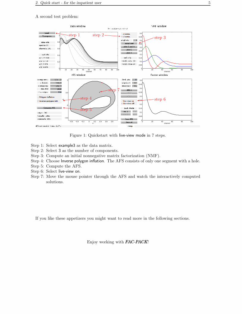
Figure 1: Quickstart with live-view mode in 7 steps.

Step 1: Select example3 as the data matrix.Step 2: Select 3 as the number of components.Step 3: Compute an initial nonnegative matrix factorization (NMF).Step 4: Choose Inverse polygon inflation. The AFS consists of only one segment with a hole.Step 5: Compute the AFS.Step 6: Select live-view on.Step 7: Move the mouse pointer through the AFS and watch the interactively computed

solutions.

If you like these appetizers you might want to read more in the following sections.

Enjoy working with FAC-PACK!

3. Introduction to FAC-PACK 6

3 Introduction to FAC-PACK

FAC-PACK is a software for the computation of nonnegative multi-component factor-izations and for the numerical approximation of the area of feasible solutions (AFS).Currently, the software can be applied to systems with s = 2 or s = 3 components.

Given a nonnegative matrix D ∈ Rk×n, which may even be perturbed in a way that some

of its entries are slightly negative, a multivariate curve resolution (MCR) technique canbe used to find nonnegative matrix factors C ∈ R

k×s and A ∈ Rs×n so that

D ≈ CA. (1)

Some references on MCR techniques are [5, 8–10, 13]. Typically the factorization (1)does not result in unique nonnegative matrix factors C and A. Instead a continuum ofpossible solutions exists [6, 10, 18]; this non-uniqueness is called the rotational ambiguityof MCR solutions. Sometimes additional information can be used to reduce this rotationalambiguity, see [7, 14] for the use of kinetic models.

The most rigorous approach is to compute the complete continuum of nonnegative matrixfactors (C,A) which satisfy (1). In 1985 Borgen and Kowalski [3] found an approach fora low dimensional representation of this continuum of solutions by the so-called areaof feasible solutions (AFS). For instance, for a three-component system (s = 3) theAFS is a two-dimensional set. Further references on the AFS are [1, 12, 17, 18]. Fora numerical computation of the AFS two methods have been developed: the triangle-boundary-enclosure scheme [4] and the polygon inflation method [16]. FAC-PACK usesthe polygon inflation method.

FAC-PACK works as follows: First the data matrix D is loaded. The singular valuedecomposition (SVD) is used to determine the number s of independent componentsunderlying the spectral data in D. FAC-PACK can be applied to systems with s = 2 ors = 3 predominating components. Noisy data is not really a problem for the algorithm asfar as the SVD is successful in separating the characteristic system data (larger singularvalues and the associated singular vectors) from the smaller noise-dependent singularvalues. Then the SVD is used to compute a low rank approximation of D. After this aninitial nonnegative matrix factorization (NMF) is computed from the low rank approxi-mation of D. This NMF is the starting point for the polygon inflation algorithm since itsupplies two or three points within the AFS. From these points an initial polygon can beconstructed, which is a first coarse approximation of the AFS. The initial polygon is in-flated to the AFS by means of an adaptive algorithm. This algorithm allows to computeall three segments of an AFS separately. Sometimes the AFS is a single topologicallyconnected set with a hole. Then an "inverse polygon inflation" scheme is applied. Theprogram allows to compute from the AFS the continuum of admissible spectra. The con-centration profiles can be computed if the whole algorithm is applied to the transposeddata matrix DT .

FAC-PACK provides a live-view mode which allows an interactive visual inspection ofthe spectra (or concentration profiles) while moving the mouse pointer through the AFS.

3. Introduction to FAC-PACK 7

Within the live-view mode the user might want to lock a certain point of the AFS, forinstance, if a known spectrum has been found. Then a reduced and smaller AFS canbe computed, which makes use of the fact that one spectrum is locked. For a three-component system this locking-and-AFS-reduction can be applied to a second point ofthe AFS.

4. Get ready to start 8

4 Get ready to start

Please download FAC-PACK from

http://www.math.uni-rostock.de/facpack/

Then extract the file FACPACK.zip. Open a MatLab desktop and run facpack.m.

This software can be used for academic, research and other similar noncommercial uses.In all other cases (e.g. commercial use) please contact the authors.

FAC-PACK does not make guarantee that the software is free of errors and that it cansuccessfully be used for a particular purpose.

4.1 Program structure

The graphical user interface of FAC-PACK is written in MatLab. The main file isPolygonInflation.m which handles all functionalities in a joint GUI. No additional MatLab

toolboxes are required to run FAC-PACK.

The GUI is built around four windows:

1. Data window (Upper-left window): The data window shows the k rows (spectra)

of the data matrix D ∈ Rk×n in a 2D-plot. The number of spectra k is printed

together with the number of spectral channels n. The four largest singular valuesof D are shown. By transposing the data matrix D it is possible to compute theAFS for the concentration factor C (instead of the AFS for the spectral factor A).

2. NMF window (Upper-right window): This window allows to set the number of com-ponents to s = 2 or s = 3 and to compute an initial NMF. The smallest minimalcomponents of C and A are printed. The figure shows the profiles of the so-calledabstract matrix factors. The buttons allow to compute the profiles of C and/or A.

3. AFS window (Lower-left window): Various control parameters allow to make cer-tain settings for the AFS computation in order to control the approximation qualityor maximal number of edges. Pressing the Compute AFS button starts the AFScomputation. The live-view mode is active after the AFS has been drawn. Justmove the mouse pointer to (and through) the AFS.

4. Factor window (Lower-right window): This window shows the spectral factors (orconcentration profiles if the transpose option has been activated in the first window)for the grid points shown in the AFS window.

4.2 External C-routine 9

4.2 External C-routine

All time-consuming numerical computations are externalized to a C-routine in order toaccelerate FAC-PACK. This C-routine is AFScomputationSYSTEMNAME.exe, whereinSYSTEMNAME stands for your system including the bit-version. For example AFScom-putationWINDOWS64.exe is used on a 64 bit windows system. The external routine iscalled if any of the buttons Initial nmf (13), Compute AFS (26), no. 1 (40) or no.

2 (42) is pressed. Pre-compiled version of the C-routine for the following systems areparts of the FAC-PACK distribution:

- Windows 32/64 bit,

- Unix 32/64 bit and

- Mac 64 bit.

The execution of the external routine can always be stopped by CTRL + C in the com-mand window. If the C-routine is running and takes too much computation time, thereason for this can be too large values for k, n, max fcls (23) or max edges (24) or toosmall values for ε-bound (21) or δ-stopping (22).

4.3 Further included libraries

The C-routine AFScomputationSYSTEMNAME.exe includes the netlib library lapack andthe ACM routine nl2sol. Any use of FAC-PACK must respectthe lapack license, see http://www.netlib.org/lapack/LICENSE.txt, andthe nl2sol license, see http://www.acm.org/publications/policies/softwarecrnotice.

5. Warming-up: Initial steps 10

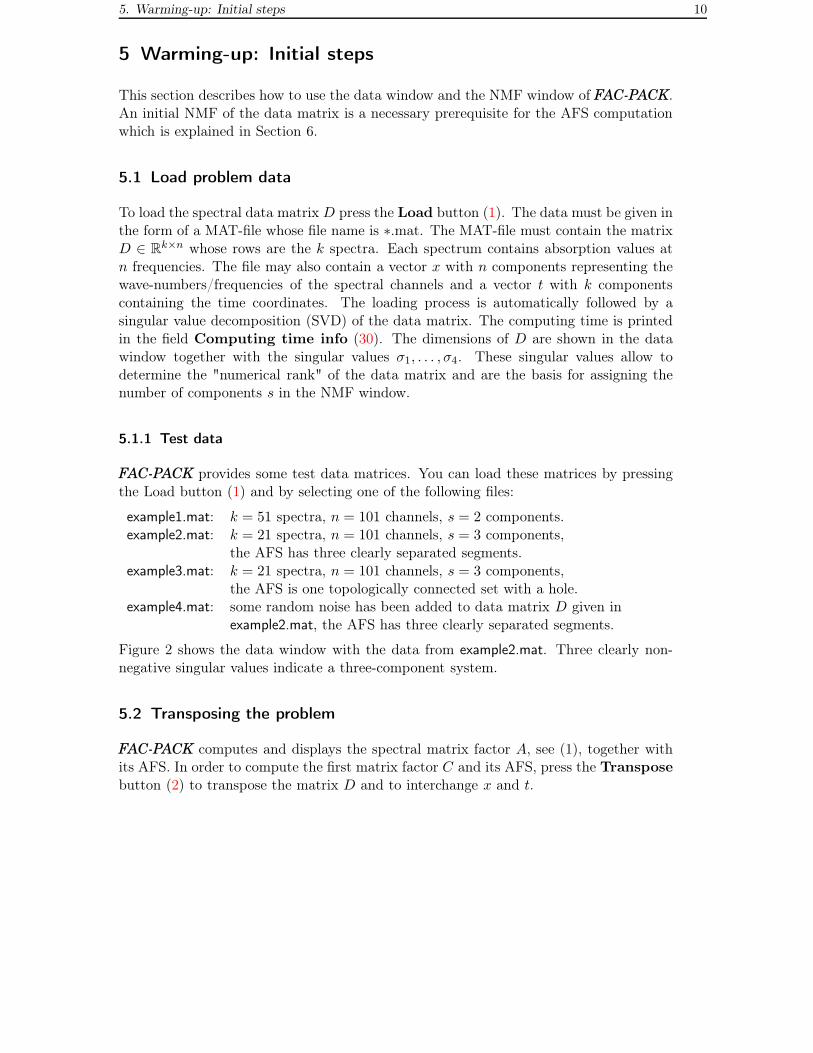
5 Warming-up: Initial steps

This section describes how to use the data window and the NMF window of FAC-PACK.An initial NMF of the data matrix is a necessary prerequisite for the AFS computationwhich is explained in Section 6.

5.1 Load problem data

To load the spectral data matrix D press the Load button (1). The data must be given inthe form of a MAT-file whose file name is ∗.mat. The MAT-file must contain the matrixD ∈ R

k×n whose rows are the k spectra. Each spectrum contains absorption values atn frequencies. The file may also contain a vector x with n components representing thewave-numbers/frequencies of the spectral channels and a vector t with k componentscontaining the time coordinates. The loading process is automatically followed by asingular value decomposition (SVD) of the data matrix. The computing time is printedin the field Computing time info (30). The dimensions of D are shown in the datawindow together with the singular values σ1, . . . , σ4. These singular values allow todetermine the "numerical rank" of the data matrix and are the basis for assigning thenumber of components s in the NMF window.

5.1.1 Test data

FAC-PACK provides some test data matrices. You can load these matrices by pressingthe Load button (1) and by selecting one of the following files:

example1.mat: k = 51 spectra, n = 101 channels, s = 2 components.example2.mat: k = 21 spectra, n = 101 channels, s = 3 components,

the AFS has three clearly separated segments.example3.mat: k = 21 spectra, n = 101 channels, s = 3 components,

the AFS is one topologically connected set with a hole.example4.mat: some random noise has been added to data matrix D given in

example2.mat, the AFS has three clearly separated segments.

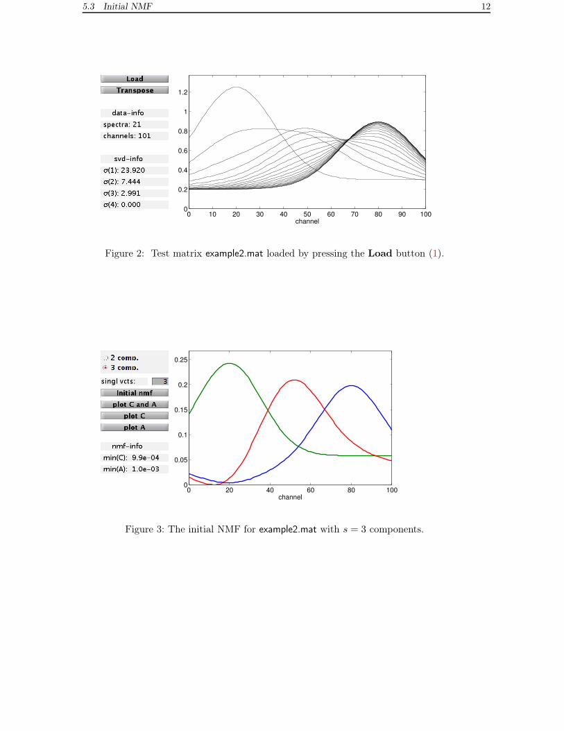
Figure 2 shows the data window with the data from example2.mat. Three clearly non-negative singular values indicate a three-component system.

5.2 Transposing the problem

FAC-PACK computes and displays the spectral matrix factor A, see (1), together withits AFS. In order to compute the first matrix factor C and its AFS, press the Transpose

button (2) to transpose the matrix D and to interchange x and t.

5.3 Initial NMF 11

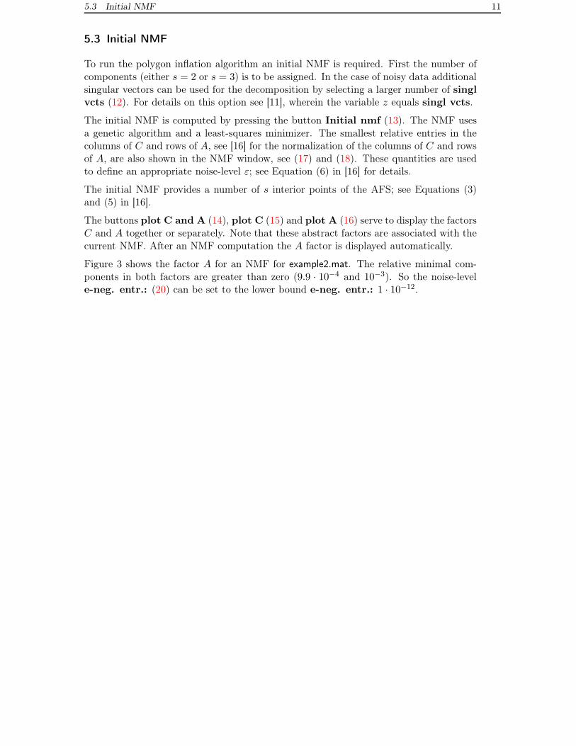
5.3 Initial NMF

To run the polygon inflation algorithm an initial NMF is required. First the number ofcomponents (either s = 2 or s = 3) is to be assigned. In the case of noisy data additionalsingular vectors can be used for the decomposition by selecting a larger number of singl

vcts (12). For details on this option see [11], wherein the variable z equals singl vcts.

The initial NMF is computed by pressing the button Initial nmf (13). The NMF usesa genetic algorithm and a least-squares minimizer. The smallest relative entries in thecolumns of C and rows of A, see [16] for the normalization of the columns of C and rowsof A, are also shown in the NMF window, see (17) and (18). These quantities are usedto define an appropriate noise-level ε; see Equation (6) in [16] for details.

The initial NMF provides a number of s interior points of the AFS; see Equations (3)and (5) in [16].

The buttons plot C and A (14), plot C (15) and plot A (16) serve to display the factorsC and A together or separately. Note that these abstract factors are associated with thecurrent NMF. After an NMF computation the A factor is displayed automatically.

Figure 3 shows the factor A for an NMF for example2.mat. The relative minimal com-ponents in both factors are greater than zero (9.9 · 10−4 and 10−3). So the noise-levele-neg. entr.: (20) can be set to the lower bound e-neg. entr.: 1 · 10−12.

5.3 Initial NMF 12

0 10 20 30 40 50 60 70 80 90 1000

0.2

0.4

0.6

0.8

1

1.2

channel

Figure 2: Test matrix example2.mat loaded by pressing the Load button (1).

0 20 40 60 80 1000

0.05

0.1

0.15

0.2

0.25

channel

Figure 3: The initial NMF for example2.mat with s = 3 components.

6. Computation of the AFS 13

6 Computation of the AFS

For two-component systems (s = 2) FAC-PACK represents the AFS by rectangles. Theirrectangular sides are the intervals of admissible values for α and β where

T =

(

1 α

1 β

)

is the transformation matrix which constitutes the rotational ambiguity. See [1, 2] forthe AFS for the case s = 2. However in [1], see Equation (6), the entries of the secondrow of T are interchanged.

For three-component systems (s = 3) the AFS is formed by all points (α, β) so that

T =

1 α β

1 s11 s121 s21 s22

is a transformation which is associated with nonnegative factors C and A, see [16]. Apermutation argument shows that with (α, β) the points (s11, s12) and (s21, s22) belongto the AFS, too.

The initial NMF is the starting point for the numerical computation of the AFS since itprovides first α and β in the AFS.

Next various control parameters for the numerical computation of the AFS are explained.Further two ways of computing different kinds of the AFS are introduced.

6.1 Control parameters

Five control parameters are used to steer the adaptive polygon inflation algorithm. FAC-

PACK aims at the best possible approximation of the AFS with the smallest computa-tional costs. Default values are pre-given for these control parameters.

• The parameter e-neg. entr. (20) is the noise level control parameter which isdenoted by ε in [16]. Negative matrix elements of C and A do not contribute tothe penalization functional if their relative magnitude is larger than −ε. In otherwords, an NMF with such slightly nonnegative matrix elements is accepted as valid.

• The parameter e-bound (21) controls the precision of the boundary approximationand is denoted by εb in [16]. Decreasing the value εb improves the accuracy of thepositioning of new vertices of the polygon.

• The parameter d-stopping (22) controls the termination of the adaptive polygoninflation procedure. This parameter is denoted by δ in Section 3.5 of [16] and isan upper bound for change-of-area which can be gained by a further subdivision ofany of the edges of the polygon.

6.2 Type of polygon inflation 14

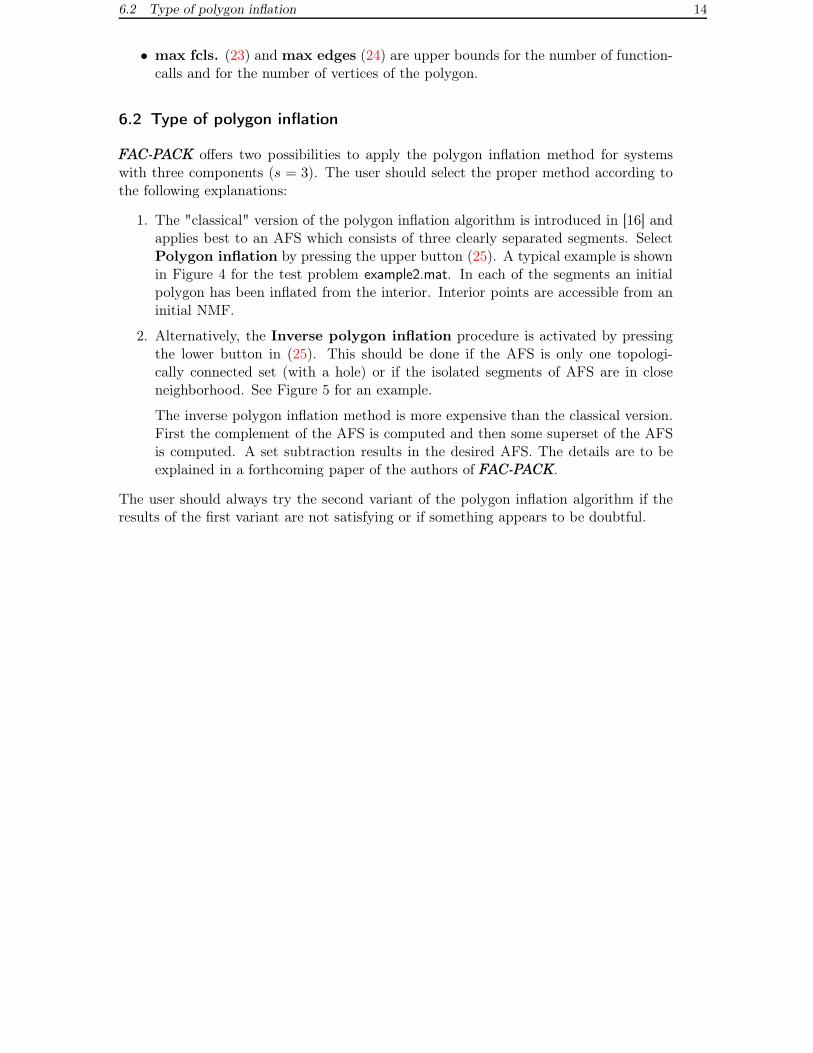
• max fcls. (23) and max edges (24) are upper bounds for the number of function-calls and for the number of vertices of the polygon.

6.2 Type of polygon inflation

FAC-PACK offers two possibilities to apply the polygon inflation method for systemswith three components (s = 3). The user should select the proper method according tothe following explanations:

1. The "classical" version of the polygon inflation algorithm is introduced in [16] andapplies best to an AFS which consists of three clearly separated segments. SelectPolygon inflation by pressing the upper button (25). A typical example is shownin Figure 4 for the test problem example2.mat. In each of the segments an initialpolygon has been inflated from the interior. Interior points are accessible from aninitial NMF.

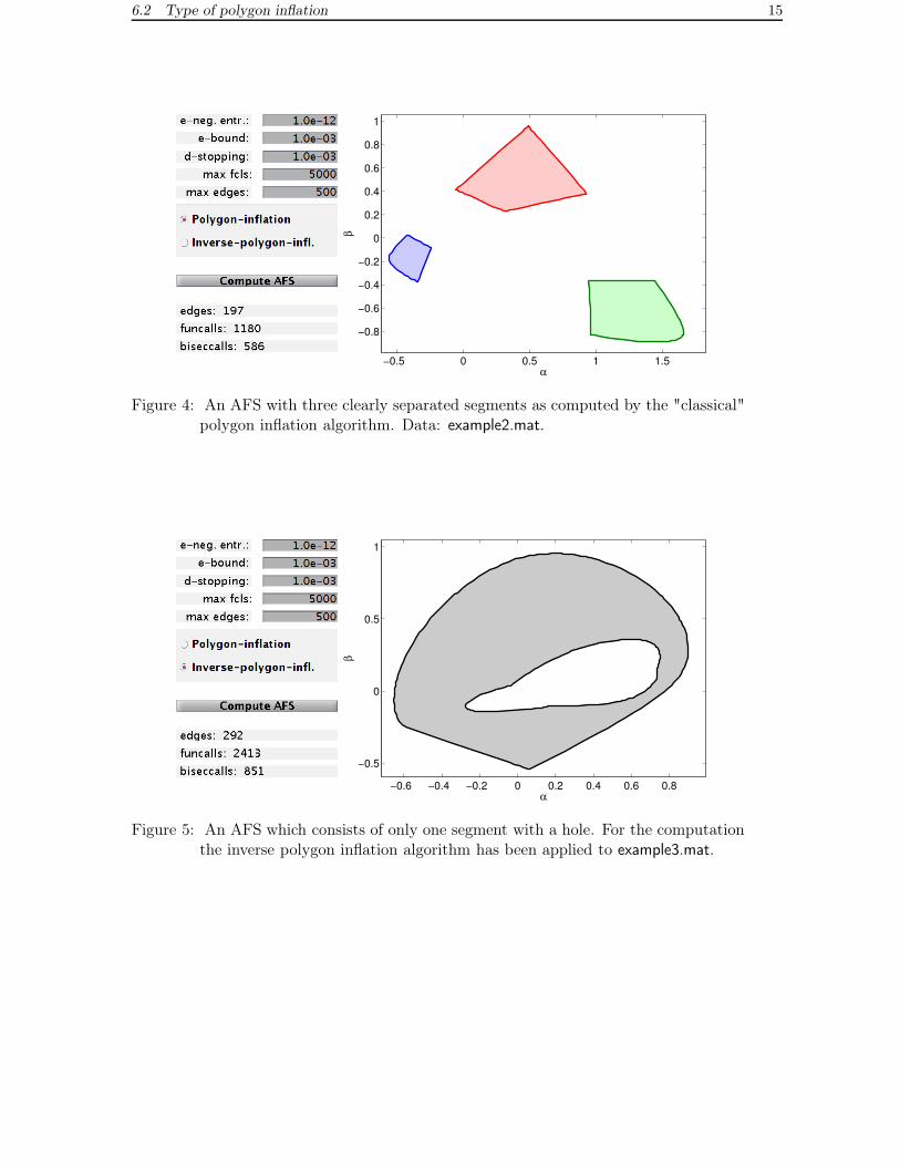
2. Alternatively, the Inverse polygon inflation procedure is activated by pressingthe lower button in (25). This should be done if the AFS is only one topologi-cally connected set (with a hole) or if the isolated segments of AFS are in closeneighborhood. See Figure 5 for an example.

The inverse polygon inflation method is more expensive than the classical version.First the complement of the AFS is computed and then some superset of the AFSis computed. A set subtraction results in the desired AFS. The details are to beexplained in a forthcoming paper of the authors of FAC-PACK.

The user should always try the second variant of the polygon inflation algorithm if theresults of the first variant are not satisfying or if something appears to be doubtful.

6.2 Type of polygon inflation 15

−0.5 0 0.5 1 1.5

−0.8

−0.6

−0.4

−0.2

0

0.2

0.4

0.6

0.8

1

α

β

Figure 4: An AFS with three clearly separated segments as computed by the "classical"polygon inflation algorithm. Data: example2.mat.

−0.6 −0.4 −0.2 0 0.2 0.4 0.6 0.8

−0.5

0

0.5

1

α

β

Figure 5: An AFS which consists of only one segment with a hole. For the computationthe inverse polygon inflation algorithm has been applied to example3.mat.

7. Factor representation & live-view mode 16

7 Factor representation & live-view mode

Next the plotting of the spectra and/or concentration profiles is described. These factorscan be computed from the AFS by certain linear combinations of the right and/or leftsingular vectors. The live-view mode allows an interactive representation of the factorsby moving the mouse pointer through the AFS.

7.1 Two-component systems

For two-component systems a full and simultaneous representation of the factors C and A

is possible. In order to get an overview of the range of possible spectra one can discretizethe AFS-intervals equidistantly. For each point of the resulting 2D discrete grid theassociated spectral line is plotted in the factor window. The discretization parameter(subinterval length) is selected in the field (33) and/or (34). The plot of the spectra isactivated by pressing button AFS 1 (35) or button AFS 2 (36).

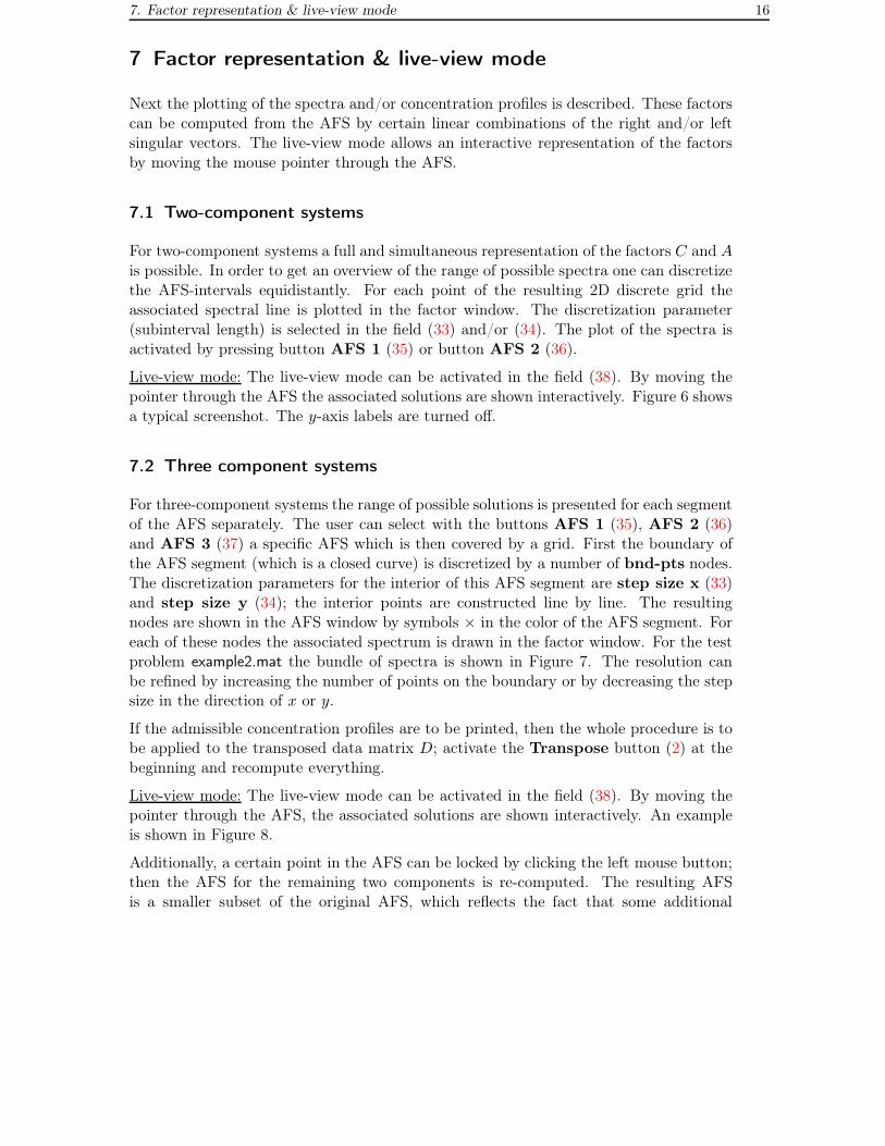
Live-view mode: The live-view mode can be activated in the field (38). By moving thepointer through the AFS the associated solutions are shown interactively. Figure 6 showsa typical screenshot. The y-axis labels are turned off.

7.2 Three component systems

For three-component systems the range of possible solutions is presented for each segmentof the AFS separately. The user can select with the buttons AFS 1 (35), AFS 2 (36)and AFS 3 (37) a specific AFS which is then covered by a grid. First the boundary ofthe AFS segment (which is a closed curve) is discretized by a number of bnd-pts nodes.The discretization parameters for the interior of this AFS segment are step size x (33)and step size y (34); the interior points are constructed line by line. The resultingnodes are shown in the AFS window by symbols × in the color of the AFS segment. Foreach of these nodes the associated spectrum is drawn in the factor window. For the testproblem example2.mat the bundle of spectra is shown in Figure 7. The resolution canbe refined by increasing the number of points on the boundary or by decreasing the stepsize in the direction of x or y.

If the admissible concentration profiles are to be printed, then the whole procedure is tobe applied to the transposed data matrix D; activate the Transpose button (2) at thebeginning and recompute everything.

Live-view mode: The live-view mode can be activated in the field (38). By moving thepointer through the AFS, the associated solutions are shown interactively. An exampleis shown in Figure 8.

Additionally, a certain point in the AFS can be locked by clicking the left mouse button;then the AFS for the remaining two components is re-computed. The resulting AFSis a smaller subset of the original AFS, which reflects the fact that some additional

7.2 Three component systems 17

0 20 40 60 80 1000

channel / time

Figure 6: The live-view mode for the two-component system example1.mat. By movingthe mouse pointer through the AFS the transformation to the factors C and A

is computed interactively and all results are plotted in the factor window. Thespectra are drawn by solid lines and the concentration profiles are representedby dash-dotted lines.

−0.5 0 0.5 1 1.5

−0.5

0

0.5

1

α

β

AFS

0 20 40 60 80 1000

0.05

0.1

0.15

0.2

channel

Solution

Figure 7: The AFS for the problem example2.mat consists of three separated segments.The blue segment of the AFS is covered with grid points (dark blue points). Foreach of these points the associated spectral line is plotted in the right figure.

−0.5 0 0.5 1 1.5

−0.5

0

0.5

1

α

β

AFS

0 20 40 60 80 1000

0.1

0.2

0.3

0.4

channel

Solution

(x,y) = (0.9896, −0.4196)

Figure 8: The live-view mode is active for the 3 component system example2.mat. In thegreen AFS-segment the mouse pointer is positioned in the left upper corner atthe coordinates (0.9896,−0.4196). The associated spectrum is shown in theright figure together with the mouse pointer coordinates.

8. Reduction of the rotational ambiguity 18

information is added by locking a certain point of the AFS. See Section 8 for furtherexplanations.

8 Reduction of the rotational ambiguity

With the computation of the AFS FAC-PACK provides a continuum of admissible matrixfactorizations. All these factorizations are mathematically correct in the sense that theyrepresent nonnegative matrix factors, whose product reproduces the original data matrixD. However, the user aims at the one solution which is believed to represent the chemicalsystem correctly. Additional information on the system can help to reduce the so-calledrotational ambiguity. FAC-PACK supports the user in this way. If, for instance onespectrum within the continuum of possible spectra is detected, which can be associatedwith a known chemical compound, then this spectrum can be locked and the resultingrestrictions can be used to reduce the AFS for the remaining components.

8.1 Locking a first spectrum

After computing the AFS, activate the live-view mode (38). While moving the mousepointer through any segment of the AFS, the factor window shows the associated spectra.If a certain (known) spectrum is found, then the user can lock this spectrum by clickingthe left mouse button. A × is plotted into the AFS and the button no. 1 (39) becomesactive. By pressing this button a smaller subset of the original AFS is drawn by solidblack lines in the AFS window. This smaller AFS reflects the fact that some additionalinformation on the system has been added. The button esc (40) can be used for unlockingany previously locked point.

8.2 Locking a second spectrum

Having locked a first spectrum and having computed the reduced AFS the live-view

mode can be reactivated. Then a second point within the reduced AFS can be locked.By pressing button no. 2 (41) the AFS for the remaining component is reduced for asecond time and is shown as a black broken line. Once again, the button esc (42) canbe used for unlocking the second point.

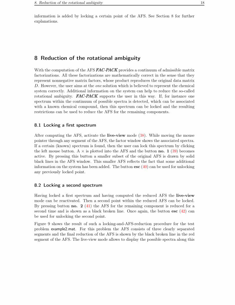
Figure 9 shows the result of such a locking-and-AFS-reduction procedure for the testproblem example2.mat. For this problem the AFS consists of three clearly separatedsegments and the final reduction of the AFS is shown by the black broken line in the redsegment of the AFS. The live-view mode allows to display the possible spectra along this

8.2 Locking a second spectrum 19

−0.5 0 0.5 1 1.5

−0.5

0

0.5

1

α

β

AFS

−0.5 0 0.5 1 1.5

−0.5

0

0.5

1

α

β

AFS

Figure 9: Reduction of the AFS for the test problem example2.mat. Left: the reducedAFS is shown by black solid lines after locking a first spectrum (marker ×).Right: The AFS of the remaining third component is shown by a black brokenline.

line. Here we do not show the resulting restrictions on the complementary concentrationfactor C; this will be the topic of some future work, cf. [15].

9. Appendix 20

9 Appendix

9.1 Save data and extract axes

To save the results in a MatLab *.mat file press either Save AFS (43) or Save all

(44). A proper file name is suggested.

Save AFS saves the data D, the factors U , S, V of the singular value decomposition,the factors Cinit, Ainit of the initial NMF and the AFS. The AFS has the data formatof a structure which contains the following variables:

• For s = 2 the AFS consists of two segments: AFS{1} ∈ R2 and AFS{2} ∈ R

2

with α ∈ [AFS{1}(1), AFS{1}(2)] and β ∈ [AFS{2}(1), AFS{2}(2)] and viceversa.

• For s = 3 and an AFS consisting of three segments: AFS{i} ∈ Rmi×2 with i =

1, 2, 3 is a polygon whose x-coordinates are AFS{i}(:, 1) and whose y-coordinatesare AFS{i}(:, 2).

• For s = 3 and an AFS consisting of one segment with a hole: AFS{1} ∈ Rm×2 is the

outer polygon (AFS{1}(:, 1) the x-coordinates and AFS{1}(:, 2) the y-coordinates)and AFS{2} ∈ R

ℓ×2 is the inner polygon surrounding the hole.

If the lock-mode has been used, see Section 8, then the results are saved in AFSLockMode1and LockPoint2 (case of one locked spectrum) as well as AFSLockMode2 and LockPoint1(case of two locked spectra).

The user can get access to all figures. Therefore click the right mouse button in thedesired figure. Then a separate MatLab figure opens. The figure can now be modified,printed or exported in the usual way.

9.2 Cancellation of the program

Whenever the buttons Initial nmf (13), Compute AFS (26), no. 1 (40) or no. 2

(42) are pressed, an external C-routine is called, see Section 4.2. The GUI does notrespond during the execution of the C-routine. Therefore, in case of any problems or incase of too long program runtimes, the C-routine cannot be canceled from the GUI. Thetermination can be enforced by typing CTRL + C in the MatLab command window.Time consuming processes can be avoided if all the parameters are adjusted to reasonable(default) values.

9.3 How to get help

If the Help box (45) is checked and the mouse pointer is moved over a button, a textfield or an axis, then a short explanation appears right next to Help field. Further, asmall pop-up window opens if the mouse pointer rests for more than one second on a

References 21

button.

References

[1] H. Abdollahi, M. Maeder, and R. Tauler, Calculation and Meaning of Feasible BandBoundaries in Multivariate Curve Resolution of a Two-Component System, Analyt-ical Chemistry 81 (2009), no. 6, 2115–2122.

[2] H. Abdollahi and R. Tauler, Uniqueness and rotation ambiguities in MultivariateCurve Resolution methods, Chemometrics and Intelligent Laboratory Systems 108

(2011), no. 2, 100–111.

[3] O.S. Borgen and B.R. Kowalski, An extension of the multivariate component-resolution method to three components, Analytica Chimica Acta 174 (1985), 1–26.

[4] A. Golshan, H. Abdollahi, and M. Maeder, Resolution of Rotational Ambiguity forThree-Component Systems, Analytical Chemistry 83 (2011), no. 3, 836–841.

[5] J.C. Hamilton and P.J. Gemperline, Mixture analysis using factor analysis. II: Self-modeling curve resolution, J. Chemometrics 4 (1990), no. 1, 1–13.

[6] J. Jaumot and R. Tauler, MCR-BANDS: A user friendly MATLAB program for theevaluation of rotation ambiguities in Multivariate Curve Resolution, Chemometricsand Intelligent Laboratory Systems 103 (2010), no. 2, 96–107.

[7] A. Juan, M. Maeder, M. Martínez, and R. Tauler, Combining hard and soft-modellingto solve kinetic problems, Chemometr. Intell. Lab. 54 (2000), 123–141.

[8] W.H. Lawton and E.A. Sylvestre, Self modelling curve resolution, Technometrics 13

(1971), 617–633.

[9] M. Maeder and Y.M. Neuhold, Practical data analysis in chemistry, Elsevier, Ams-terdam, 2007.

[10] E. Malinowski, Factor analysis in chemistry, Wiley, New York, 2002.

[11] K. Neymeyr, M. Sawall, and D. Hess, Pure component spectral recovery and con-strained matrix factorizations: Concepts and applications, J. Chemometrics 24

(2010), 67–74.

[12] R. Rajkó and K. István, Analytical solution for determining feasible regions of self-modeling curve resolution (SMCR) method based on computational geometry, J.Chemometrics 19 (2005), no. 8, 448–463.

[13] C. Ruckebusch and L. Blanchet, Multivariate curve resolution: A review of advancedand tailored applications and challenges, Analytica Chimica Acta 765 (2013), 28–36.

[14] M. Sawall, A. Börner, C. Kubis, D. Selent, R. Ludwig, and K. Neymeyr, Model-free multivariate curve resolution combined with model-based kinetics: algorithm andapplications, J. Chemometrics 26 (2012), 538–548.

References 22

[15] M. Sawall, C. Fischer, D. Heller, and K. Neymeyr, Reduction of the rotational am-biguity of curve resolution technqiues under partial knowledge of the factors. Com-plementarity and coupling theorems, J. Chemometrics 26 (2012), 526–537.

[16] M. Sawall, C. Kubis, D. Selent, A. Börner, and K. Neymeyr, A fast polygon inflationalgorithm to compute the area of feasible solutions for three-component systems. I:Concepts and applications, J. Chemometrics 27 (2013), 106–116.

[17] R. Tauler, Calculation of maximum and minimum band boundaries of feasible solu-tions for species profiles obtained by multivariate curve resolution, J. Chemometrics15 (2001), no. 8, 627–646.

[18] M. Vosough, C. Mason, R. Tauler, M. Jalali-Heravi, and M. Maeder, On rotationalambiguity in model-free analyses of multivariate data, J. Chemometrics 20 (2006),no. 6-7, 302–310.