
Universit a degli Studi di Siena Facolt a di Scienze ... · x Introduction (charged lepton,...
173
Universit` a degli Studi di Siena Facolt` a di Scienze Matematiche Fisiche e Naturali Tesi di Dottorato in Fisica Sperimentale PhD Thesis in Experimental Physics XXIII Ciclo Measurement of WW + WZ Production Cross Section and Study of the Dijet Mass Spectrum in the ‘ν + jets Final State at CDF Candidate Advisor Viviana Cavaliere Dott. Maria Agnese Ciocci
Transcript of Universit a degli Studi di Siena Facolt a di Scienze ... · x Introduction (charged lepton,...
Universita degli Studi di Siena
Facolta di Scienze Matematiche Fisiche e Naturali
Tesi di Dottorato in Fisica Sperimentale
PhD Thesis in Experimental Physics
XXIII Ciclo
Measurement of WW +WZ Production
Cross Section and Study of the Dijet Mass
Spectrum in the `ν + jets Final State at CDF
Candidate Advisor
Viviana Cavaliere Dott. Maria Agnese Ciocci


A mamma, papa e Ale

ii
Contents
Abstract vii
Introduction ix
1 Theoretical Overview and Motivation 1
1.1 The Standard Model . . . . . . . . . . . . . . . . . . . . . . . . . . . 1
1.2 Electroweak Sector and the Higgs Mechanism . . . . . . . . . . . . . 4
1.2.1 Beyond the Standard Model . . . . . . . . . . . . . . . . . . . 5
1.3 WW and WZ Production and Decay . . . . . . . . . . . . . . . . . . 6
1.4 Main Challenges and Motivations . . . . . . . . . . . . . . . . . . . . 8
1.5 Status of Diboson Measurements . . . . . . . . . . . . . . . . . . . . 11
2 Experimental Apparatus 13
2.1 The Tevatron Collider . . . . . . . . . . . . . . . . . . . . . . . . . . 13
2.1.1 Proton Production . . . . . . . . . . . . . . . . . . . . . . . . 13
2.1.2 Antiproton Production . . . . . . . . . . . . . . . . . . . . . . 14
2.1.3 Tevatron . . . . . . . . . . . . . . . . . . . . . . . . . . . . . 15
2.2 Luminosity . . . . . . . . . . . . . . . . . . . . . . . . . . . . . . . . 16
2.3 CDF Run II detector . . . . . . . . . . . . . . . . . . . . . . . . . . . 17
2.3.1 Coordinate System and Useful Variables . . . . . . . . . . . . 19
2.3.2 Tracking . . . . . . . . . . . . . . . . . . . . . . . . . . . . . . 20
2.3.3 Time of Flight . . . . . . . . . . . . . . . . . . . . . . . . . . 24
2.3.4 Calorimeter System . . . . . . . . . . . . . . . . . . . . . . . 24
2.3.5 Shower Profile Detectors . . . . . . . . . . . . . . . . . . . . . 27
iii
iv Contents
2.3.6 Muons System . . . . . . . . . . . . . . . . . . . . . . . . . . 27
2.3.7 CLC and Measurement of the Luminosity . . . . . . . . . . . 30
2.4 Trigger and Data Acquisition . . . . . . . . . . . . . . . . . . . . . . 31
2.4.1 Level 1 Trigger . . . . . . . . . . . . . . . . . . . . . . . . . . 32
2.4.2 Level 2 Trigger . . . . . . . . . . . . . . . . . . . . . . . . . . 33
2.4.3 Level 3 Trigger . . . . . . . . . . . . . . . . . . . . . . . . . . 35
3 Objects Identification and Event Reconstruction 37
3.1 High Level Detector Objects . . . . . . . . . . . . . . . . . . . . . . . 37
3.1.1 Tracking . . . . . . . . . . . . . . . . . . . . . . . . . . . . . . 37
3.1.2 Primary Vertex . . . . . . . . . . . . . . . . . . . . . . . . . . 39
3.1.3 Calorimeter Clusters . . . . . . . . . . . . . . . . . . . . . . . 39
3.2 Physical Objects . . . . . . . . . . . . . . . . . . . . . . . . . . . . . 40
3.2.1 Electrons . . . . . . . . . . . . . . . . . . . . . . . . . . . . . 40
3.2.2 Muons . . . . . . . . . . . . . . . . . . . . . . . . . . . . . . . 42
3.2.3 Jets . . . . . . . . . . . . . . . . . . . . . . . . . . . . . . . . 45
3.2.4 Missing Transverse Energy . . . . . . . . . . . . . . . . . . . 50
4 Event Selection 53
4.1 Signal and Background Definition . . . . . . . . . . . . . . . . . . . . 53
4.2 Data Sample . . . . . . . . . . . . . . . . . . . . . . . . . . . . . . . 56
4.3 Trigger Requirements . . . . . . . . . . . . . . . . . . . . . . . . . . 57
4.3.1 Central Electron Trigger . . . . . . . . . . . . . . . . . . . . . 57
4.3.2 Central Muon Trigger . . . . . . . . . . . . . . . . . . . . . . 58
4.4 Leptonic W Candidate . . . . . . . . . . . . . . . . . . . . . . . . . . 59
4.5 Hadronic W/Z Candidate . . . . . . . . . . . . . . . . . . . . . . . . 61
5 Sample Composition and Modeling 63
5.1 MC-Based Processes . . . . . . . . . . . . . . . . . . . . . . . . . . . 63
5.1.1 Diboson . . . . . . . . . . . . . . . . . . . . . . . . . . . . . . 64
5.1.2 W+jets . . . . . . . . . . . . . . . . . . . . . . . . . . . . . . 65
5.1.3 Z+jets . . . . . . . . . . . . . . . . . . . . . . . . . . . . . . . 67
iv
Contents v
5.1.4 tt and single top production . . . . . . . . . . . . . . . . . . . 67
5.2 Data-Driven Background Modeling . . . . . . . . . . . . . . . . . . . 67
5.3 Instantaneous Luminosity Correction . . . . . . . . . . . . . . . . . . 69
5.4 Dijet Mass Shape . . . . . . . . . . . . . . . . . . . . . . . . . . . . . 70
5.5 Modeling Validation . . . . . . . . . . . . . . . . . . . . . . . . . . . 73
6 Fit Description and Validation 79
6.1 Fit Procedure . . . . . . . . . . . . . . . . . . . . . . . . . . . . . . 79
6.2 Fitter Validation . . . . . . . . . . . . . . . . . . . . . . . . . . . . . 83
7 Results 85
7.1 Fit Results on Data . . . . . . . . . . . . . . . . . . . . . . . . . . . 85
7.2 Systematic Uncertainties . . . . . . . . . . . . . . . . . . . . . . . . . 87
7.2.1 Signal Extraction . . . . . . . . . . . . . . . . . . . . . . . . . 87
7.2.2 Cross-Section Evaluation . . . . . . . . . . . . . . . . . . . . 93
7.3 Final Results and Significance Estimation . . . . . . . . . . . . . . . 94
8 Study of the Dijet Mass Spectrum 99
8.1 Event Selection and Preliminary Background Estimate . . . . . . . . 99
8.2 Background Modeling Studies . . . . . . . . . . . . . . . . . . . . . . 101
8.2.1 QCD Background . . . . . . . . . . . . . . . . . . . . . . . . 110
8.2.2 W+jets studies . . . . . . . . . . . . . . . . . . . . . . . . . . 114
8.2.3 ∆Rjj Modeling . . . . . . . . . . . . . . . . . . . . . . . . . . 115
9 Search for a Dijet Resonance 119
9.1 Strategy . . . . . . . . . . . . . . . . . . . . . . . . . . . . . . . . . . 119
9.1.1 Fitting Procedure . . . . . . . . . . . . . . . . . . . . . . . . 120
9.2 Fit to the Data . . . . . . . . . . . . . . . . . . . . . . . . . . . . . . 123
9.3 Systematic and Significance . . . . . . . . . . . . . . . . . . . . . . . 126
9.4 Additional Cross-Checks . . . . . . . . . . . . . . . . . . . . . . . . . 129
9.5 Final considerations . . . . . . . . . . . . . . . . . . . . . . . . . . . 132
Conclusions and Perspectives 137
v
vi Contents
Appendices 141
A Lepton Trigger and Reconstruction efficiency 143
A.1 Lepton Trigger Efficiency . . . . . . . . . . . . . . . . . . . . . . . . 143
A.2 Electron Reconstruction Efficiency . . . . . . . . . . . . . . . . . . . 144
A.3 Muon Reconstruction Efficiency . . . . . . . . . . . . . . . . . . . . . 144
A.4 CEM Electron Energy Scale Factor . . . . . . . . . . . . . . . . . . 145
B Monte Carlo Simulation 147
B.1 Parton Distribution Function . . . . . . . . . . . . . . . . . . . . . . 148
B.2 Event Generation . . . . . . . . . . . . . . . . . . . . . . . . . . . . . 148
B.2.1 PYTHIA . . . . . . . . . . . . . . . . . . . . . . . . . . . . . . 149
B.2.2 MADEVENT . . . . . . . . . . . . . . . . . . . . . . . . . . . . . 150
B.2.3 ALPGEN . . . . . . . . . . . . . . . . . . . . . . . . . . . . . . 150
B.3 Showering . . . . . . . . . . . . . . . . . . . . . . . . . . . . . . . . . 150
B.4 Dector simulation . . . . . . . . . . . . . . . . . . . . . . . . . . . . . 151
Bibliography 153
Bibliography 153
Acknowledgements 160
vi
Abstract
We present the measurement of the WW and WZ production cross section in pp
collisions at√s = 1.96 TeV, in a final state consisting of an electron or muon,
neutrino and jets. The data analyzed were collected by the CDF II detector at the
Tevatron collider and correspond to 4.3 fb−1 of integrated luminosity.
The analysis uses a fit to the dijet mass distribution to extract the diboson con-
tribution. We observe 1582± 275(stat.)± 107(syst.) diboson candidate events and
measure a cross section of σWW/WZ = 18.1± 3.3(stat.)± 2.5(syst.) pb, consistent
with the Standard Model prediction of 15.9± 0.9 pb.
The best fit to the dijet mass of the known components shows a good agreement
with the data except for the [120, 160] GeV/c2 mass range, where an excess is
observed. We perform detailed checks of our background model and study the
significance of the excess, assuming an additional gaussian component with a width
compatible with the expected dijet mass resolution. A standard ∆χ2 test of the
presence of the additional component, returns a p-value of 4.2×10⁻⁴ when standard
sources of systematics are considered, corresponding to a significance of 3.3σ.
vii

viii Abstract
Introduction
The Standard Model of particle physics has been extensively tested in the past
decades. The analysis of the data collected by the experiments at LEP and Tevatron
colliders confirmed its predictions with an accuracy sometimes well below 1%. But,
despite all these confirmations, there is still a lot to understand: why neutrinos have
masses? What are dark matter and dark energy? Does the Higgs boson exist or, if
it does not, what is the mechanism that gives masses to the fermions and to W and
Z bosons? The experiments at both the Tevatron and the LHC colliders are now
in an excellent position to give conclusive answers to many of these open questions.
To this aim, the study of heavy diboson processes (such as WW , WZ and ZZ)
is very appealing as they are a direct probe of the gauge structure of the Standard
Model. Their cross section could be enhanced by new physics and they are sensitive
to anomalous triple gauge couplings. These processes are also the most important
and irreducible backgrounds to the Higgs searches in both the low and high mass
region.
This thesis describes the measurement, with the CDF II detector, of the cross
section of WW and WZ production in pp collisions at√s = 1.96 TeV, studying
the final state where a W decays leptonically and the second W or Z boson decays
hadronically. This channel is rather challenging in hadron colliders due to the large
background of single W produced in association with jets. However, this decay mode
has a much larger branching fraction than the cleaner fully leptonic mode and is
topologically similar to the associated production of a Higgs boson with a W . The
analysis of WW and WZ in these channels is a benchmark for the actual feasibility
of the Higgs search, and the methods used might lead to significant progress in this
sector.
The theoretical framework and motivations for this measurement are given in
Chapter 1. Chapter 2 describes the Tevatron collider and the CDF II detector.
The sophisticated algorithms used to translate the data into the physical objects
ix
x Introduction
(charged lepton, neutrino and jets) are summarized in Chapter 3 and 4. The
backgrounds (and the signal) are modeled using a Monte Carlo simulation and
data-driven techniques as explained in Chapter 5. The technique used to extract
the diboson contribution includes a fit of the dijet mass shape in the data to the
sum of the contributing processes. The fit procedure and its validation are reported
in Chapter 6. The analysis results for the WW + WZ cross section are presented
in Chapter 7.
The first measurement of this analysis, with 3.9 fb−1 of total integrated lumi-
nosity, has been published in Physical Review Letters [1]. The update to 4.3 fb−1
presented in this thesis (with just some minor changes to the fitting procedure) has
been approved by the CDF Collaboration and is available for the public in [2] and
is meant to be published in Physical Review D.
The last part of this thesis describes the effort made to understand the discrep-
ancy found between the best fit to the dijet mass of the known components and
the data in the region [120, 160] GeV/c2. We check the goodness of our background
modeling by comparing data and backgrounds in different regions of mass and with
different selections (Chapter 8). In order to quote the significance of the excess, in
Chapter 9 we make the simplest assumption, adding in the modeling of the data,
an additional gaussian component with width compatible with the expected dijet
invariant mass resolution. The fitted gaussian has a significance of 3.3σ.
The latter results are in the process of being approved by the Collaboration and
are meant to be submitted in Physical Review Letters.
Chapter 1
Theoretical Overview and
Motivation
Our current best understanding of elementary particles is summarized in the so-
called Standard Model of particles physics. Its description of particles and inter-
actions has been tested and validated across a wide range of energies in numerous
experiments. But there are still a lot of open questions, therefore the role of ex-
perimental particle physics is to test the Standard Model in all conceivable ways,
seeking to discover whether something more lies beyond it.
The following chapter provides an outline of this model, focusing the attention
on the electroweak sector and on the theoretical motivations for the measurement
of WW/WZ production, subject of this thesis.
1.1 The Standard Model
The Standard Model (SM) is a relativistic quantum field theory [3] that describes
all the elementary particles and three of the four known fundamental forces which
govern the interaction of matter: electromagnetism, strong and weak forces. Grav-
ity, is far weaker (roughly 40 orders of magnitude smaller than the strong nuclear
force) and is not expected to contribute significantly to the physical processes which
are of current interest in high energy particle physics.
In the SM, all fundamental interactions derive from a single general principle, the
requirement of local gauge invariance of the lagrangian. The gauge transformations
1
2 Chapter 1. Theoretical Overview and Motivation
that describe the natural forces belong to the unitary group:
GSM = SU(3)C ⊗ SU(2)L ⊗ U(1)Y
where the subscript stands for the conserved charges: the strong charge or color
C, the weak isospin T (or better, his third componend T3) and the hypercharge Y .
These quantities are connected to the electric charge Q (conserved too) through the
Gell-Mann–Nishijima relation:
Q =Y
2+ T3.
In this model, the elementary particles are representations of the symmetry
group GSM . They are divided in two families: fermions with spin 1/2 that satisfy
Fermi-Dirac statistics and bosons, with spin 1, that satisfy Bose-Einstein statistics.
There are 12 fundamental fermions and the corresponding anti-particles; 6 interact
just through the electroweak force and are called leptons, the others 6 interact also
through the strong force and are called quarks.
Leptons, that in the SM are massless particles, are described as doublets of
the SU(2)L group with their associate neutrinos, as eigenstates of chirality with −1
eigenvalue (left-handed eigenstates), one for each generation (e, µ, τ). As Goldhaber
[4] has experimentally proved, neutrinos with positive chirality eigenvalues do not
exists and the right-handed fermions in the SM ought to be singlets for SU(2)L:(νe
e
)L
(νµ
µ
)L
(ντ
τ
)L
(e)R (µ)R (τ)R
The quarks are the particles that interact by the strong interaction. According
to SM they are divided into left-handed doublets and right-handed singlets as lep-
tons and neutrinos:(u
d
)L
(c
s
)L
(t
b
)L
(u)R (d)R (c)R
(s)R (t)R (b)R
Quarks carry color charge, but “colored” particles have never been observed in
nature so all terms of the lagrangian must be singlets of SU(3)C , i.e. quarks have to
bind into color neutral states called hadrons, and the color charge is confined. When
highly energetic quarks or gluons are produced in high energy physics experiment
a process called hadronization or showering takes place: after a quark-antiquark
pair, or more in general a parton1, is produced in an interaction, the potential
1The word originates from Feynman who called the constituent of the proton parton, so it refers
1.1 The Standard Model 3
between them, due to gluons exchange, tries to keep them together until the strength
reaches a breaking point where further quark-antiquark pairs are created and finally
bound together with the original parton. This process involves a large number of
interactions at different scales until the scale of hadrons is reached. The process
is then essentially non-perturbative and not completely theoretically under control.
The quarks could also radiate gluons that creates other qq pairs. The final state in
which we observe the parton generated in the interaction is a collimated “jet” (see
Sec. 3.2.3) of particles approximately in the direction of the original parton.
The generators of the symmetry group GSM , i.e. the mediators of the fun-
damental interactions, are spin 1 elementary particles called gauge bosons. The
photon (γ) and three vector bosons (W± and Z) are the generators of the group
SU(2)L ⊗ U(1)Y , while the gluons (g) are the generators of the group SU(3)C .
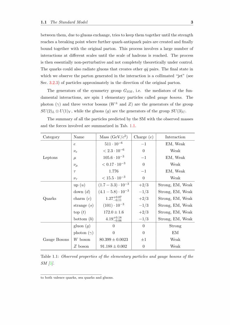
The summary of all the particles predicted by the SM with the observed masses
and the forces involved are summarized in Tab. 1.1.
Category Name Mass (GeV/c2) Charge (e) Interaction
e 511 · 10−6 −1 EM, Weak
νe < 2.3 · 10−6 0 Weak
Leptons µ 105.6 · 10−3 −1 EM, Weak
νµ < 0.17 · 10−3 0 Weak
τ 1.776 −1 EM, Weak
ντ < 15.5 · 10−3 0 Weak
up (u) (1.7− 3.3) · 10−3 +2/3 Strong, EM, Weak
down (d) (4.1− 5.8) · 10−3 −1/3 Strong, EM, Weak
Quarks charm (c) 1.27+0.07−0.11 +2/3 Strong, EM, Weak
strange (s) (101) · 10−3 −1/3 Strong, EM, Weak
top (t) 172.0± 1.6 +2/3 Strong, EM, Weak
bottom (b) 4.19+0.18−0.06 −1/3 Strong, EM, Weak
gluon (g) 0 0 Strong
photon (γ) 0 0 EM
Gauge Bosons W boson 80.399± 0.0023 ±1 Weak
Z boson 91.188± 0.002 0 Weak
Table 1.1: Observed properties of the elementary particles and gauge bosons of the
SM [5].
to both valence quarks, sea quarks and gluons.
4 Chapter 1. Theoretical Overview and Motivation
1.2 Electroweak Sector and the Higgs Mechanism
A big success of the SM is the unification of the electromagnetic and the weak forces
into the so called electroweak force [6]. The idea of the unification is to combine
both interactions into one single theoretical framework, in which they would appear
as two manifestations of the same fundamental force. If we indicate the gauge fields
and the coupling constants of the group SU(2)L ⊗ U(1)Y respectively as W iµ, Bµ,
and g, g′, the electroweak lagrangian can be written as
LEW = −1
4WµνW
µν − 1
4BµνB
µν + ψiγµDµψ (1.1)
where we used the Yang–Mills and Maxwell tensors,
Wµν = ∂µWν − ∂νWµ − gWµ ×Wν and Bµν = ∂µBν − ∂νBµ,
and the covariant derivative is defined as
Dµ = ∂µ + igWµT +1
2ig′BµY.
The first two componenets of W iµ are associated to the physical W± boson, while
the electromagnetic field, Aµ, and neutral current, Zµ, are obtained with a rotation
of an angle θW , defined by g′ = g tan θW , of the fields W 3µ and Bµ:(
Zµ
Aµ
)=
(cos θW − sin θW
sin θW cos θW
)=
(W 3µ
Bµ
)
As a result, the electric charge is e = g sin θW and the real fields are
W±µ =1√2
(W 1µ ∓ iW 2
µ) (1.2)
Zµ =−g′Bµ + gW 3
µ√g2 + g′2
(1.3)
Aµ =gBµ + g′W 3
µ√g2 + g′2
(1.4)
When we introduce the physical fields in the lagragian of eq. (1.1), from the first
term we get up to quartic interaction vertices between charged bosons or charged
and neutral bosons, while the second term produces vertices with no more than
two neutral bosons. Triple gauge couplings (or quartic interaction vertices) of only
neutral bosons such as ZZZ, ZZγ, Zγγ, are then absent in the SM.
The gauge invariance of SU(2)L ⊗ U(1)Y implies massless weak bosons and
fermions. This is in total contradiction with reality where, as shown in Tab. 1.1,
1.2 Electroweak Sector and the Higgs Mechanism 5
weak bosons (W and Z) and almost all fermions are experimentally observed to be
massive. The most accepted solution to this problem is the Higgs mechanism [7].
This mechanism predicts the existence of a scalar field, Φ, whose corresponding
lagrangian density has the form
LΦ = (DµΦ)†DµΦ− V (Φ),
where the potential is defined as
V (Φ) = µ2Φ†Φ + λ(Φ†Φ)2.
If λ > 0 and µ2 < 0 the potential has a minimum for Φ†Φ = µ2/2λ ≡ v2/2.
Thus the field Φ has a non-zero vacuum expectation value (VEV). Choosing one
of a set of degenerate states of minimum energy breaks the gauge symmetry. As
stated by the Goldstone theorem, fields that acquire a VEV will have an associated
massless boson which will disappear, transformed into the longitudinal component
of a massive gauge boson. Since the photon is known to be massless, the symmetry
is chosen to be broken so that only the fields with zero electric charge (the ones
that cannot couple to the electromagnetic interaction) acquire a VEV. Expanding
around the true minimum of the theory, the complex field Φ becomes:
Φ(x) = eiσjξj(x)/v 1√2
(0
v +H(x)
)
Here, H is the Higgs field, σj are the Pauli matrices and ξj(x) are non-physical
Goldstone bosons. When we introduce this specific representation of Φ in the SM
lagrangian, what happens is that the Goldstone bosons vanish while the gauge
bosons acquire terms which can be identified as mass terms. From the broken
lagrangian one finds the following relations between the masses of the gauge bosons:
MW = MZ cos θW and MH =√−2µ2.
Then the mass of the Higgs boson is undetermined and needs to be measured ex-
perimentally. So far, the Higgs boson has still not been observed, only experimental
limits from both LEP and the Tevatron exist [8] [9].
1.2.1 Beyond the Standard Model
Even if, at the present time, no experiment has been able to find any clear deviation
from SM predictions (with the only exception of neutrino oscillations and masses
6 Chapter 1. Theoretical Overview and Motivation
[10]) the Higgs mechanism and its use of an elementary scalar field to generate
particles masses is problematic.
In fact, in the SM there is no mechanism to prevent scalar particles from acquir-
ing large masses through radiative corrections. Therefore, M2H receives enormous
high order loop corrections from every particle which couples to the Higgs field. If
the SM has to to describe nature up to the Planck scale, then the quantum correc-
tion ∆M2H , is about 30 orders of magnitude larger than the bare Higgs mass square.
A cancellation of these corrections at all orders would call for an incredibly “fine
tuning” which seems very unlikely [11].
In a model with spontaneous electroweak symmetry breaking, the problem af-
fects not only the Higgs mass, but also its expectation value and the masses of all
other particles such as the W and Z boson, the quarks and the charged leptons.
Hence, it is unnatural to have all the SM particles masses at the electroweak scale
unless the model is somehow cut off and embedded in a richer structure at energies
no bigger than the TeV scale.
Several other theories exist such as supersymmetry (SUSY), technicolor, and
fourth-generation models to name a few, that try to solve this “hierarchy problem”.
SUSY [12] in particular, predicts bosonic super-partners for fermions (and vice-
versa) in a way that each term in ∆M2H has a counter-term that naturally cancel
all the huge corrections (since ∆M2H receives contributions with different sign from
fermions and bosons).
Technicolor [13], instead, hides electroweak symmetry and generate masses for
the W and Z bosons through the dynamics of new gauge interactions. Although
asymptotically free at very high energies, these interactions must become strong
and confining (and hence unobservable) at the lower energies that have been ex-
perimentally probed. This dynamical approach is natural and avoids the hierarchy
problem of the SM.
1.3 WW and WZ Production and Decay
Because of so many open questions about the mechanism that gives masses to the W
and Z bosons, studying their couplings and production cross sections may provide
useful information.
Moreover, one of the peculiarity of the SM is that it is a non abelian theory.
This implies that gauge bosons have auto-interactions, where vertices with three
1.3 WW and WZ Production and Decay 7
q
qγ,Z
p
p
W−
W+
q
q′
q
p
p
W+
W−
q
q′W+
p
p
Z
W+
q′
q
q
p
p
W+
Z
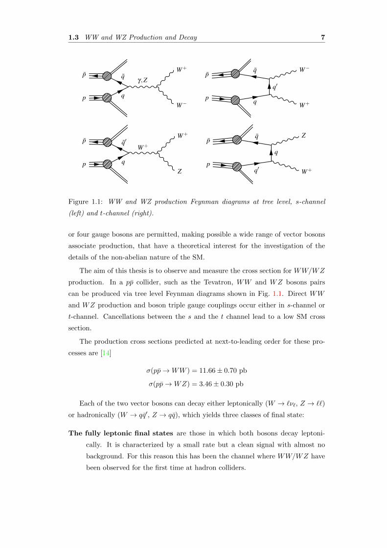
Figure 1.1: WW and WZ production Feynman diagrams at tree level, s-channel
(left) and t-channel (right).
or four gauge bosons are permitted, making possible a wide range of vector bosons
associate production, that have a theoretical interest for the investigation of the
details of the non-abelian nature of the SM.
The aim of this thesis is to observe and measure the cross section for WW/WZ
production. In a pp collider, such as the Tevatron, WW and WZ bosons pairs
can be produced via tree level Feynman diagrams shown in Fig. 1.1. Direct WW
and WZ production and boson triple gauge couplings occur either in s-channel or
t-channel. Cancellations between the s and the t channel lead to a low SM cross
section.
The production cross sections predicted at next-to-leading order for these pro-
cesses are [14]
σ(pp→WW ) = 11.66± 0.70 pb
σ(pp→WZ) = 3.46± 0.30 pb
Each of the two vector bosons can decay either leptonically (W → `ν`, Z → ``)
or hadronically (W → qq′, Z → qq), which yields three classes of final state:
The fully leptonic final states are those in which both bosons decay leptoni-
cally. It is characterized by a small rate but a clean signal with almost no
background. For this reason this has been the channel where WW/WZ have
been observed for the first time at hadron colliders.
8 Chapter 1. Theoretical Overview and Motivation
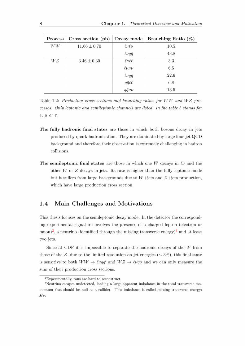
Process Cross section (pb) Decay mode Branching Ratio (%)
WW 11.66± 0.70 `ν`ν 10.5
`νqq 43.8
WZ 3.46± 0.30 `ν`` 3.3
`ννν 6.5
`νqq 22.6
qq`` 6.8
qqνν 13.5
Table 1.2: Production cross sections and branching ratios for WW and WZ pro-
cesses. Only leptonic and semileptonic channels are listed. In the table ` stands for
e, µ or τ .
The fully hadronic final states are those in which both bosons decay in jets
produced by quark hadronization. They are dominated by large four-jet QCD
background and therefore their observation is extremely challenging in hadron
collisions.
The semileptonic final states are those in which one W decays in `ν and the
other W or Z decays in jets. Its rate is higher than the fully leptonic mode
but it suffers from large backgrounds due to W+jets and Z+jets production,
which have large production cross section.
1.4 Main Challenges and Motivations
This thesis focuses on the semileptonic decay mode. In the detector the correspond-
ing experimental signature involves the presence of a charged lepton (electron or
muon)2, a neutrino (identified through the missing transverse energy)3 and at least
two jets.
Since at CDF it is impossible to separate the hadronic decays of the W from
those of the Z, due to the limited resolution on jet energies (∼ 3%), this final state
is sensitive to both WW → `νqq′ and WZ → `νqq and we can only measure the
sum of their production cross sections.
2Experimentally, taus are hard to reconstruct.3Neutrino escapes undetected, leading a large apparent imbalance in the total transverse mo-
mentum that should be null at a collider. This imbalance is called missing transverse energy:
�ET .
1.4 Main Challenges and Motivations 9
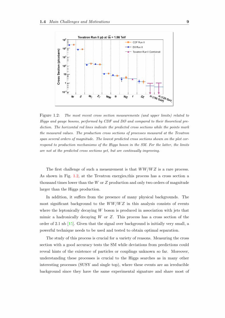
Figure 1.2: The most recent cross section measurements (and upper limits) related to
Higgs and gauge bosons, performed by CDF and DØ and compared to their theoretical pre-
diction. The horizontal red lines indicate the predicted cross sections while the points mark
the measured values. The production cross sections of processes measured at the Tevatron
span several orders of magnitude. The lowest predicted cross sections shown on the plot cor-
respond to production mechanisms of the Higgs boson in the SM. For the latter, the limits
are not at the predicted cross sections yet, but are continually improving.
The first challenge of such a measurement is that WW/WZ is a rare process.
As shown in Fig. 1.2, at the Tevatron energies,this process has a cross section a
thousand times lower than the W or Z production and only two orders of magnitude
larger than the Higgs production.
In addition, it suffers from the presence of many physical backgrounds. The
most significant background to the WW/WZ in this analysis consists of events
where the leptonically decaying W boson is produced in association with jets that
mimic a hadronically decaying W or Z. This process has a cross section of the
order of 2.1 nb [15]. Given that the signal over background is initially very small, a
powerful technique needs to be used and tested to obtain optimal separation.
The study of this process is crucial for a variety of reasons. Measuring the cross
section with a good accuracy tests the SM while deviations from predictions could
reveal hints of the existence of particles or couplings unknown so far. Moreover,
understanding these processes is crucial to the Higgs searches as in many other
interesting processes (SUSY and single top), where these events are an irreducible
background since they have the same experimental signature and share most of
10 Chapter 1. Theoretical Overview and Motivation
the trigger, Monte Carlo (MC) simulation, and analysis methods. Hence, a better
understanding of diboson production allows for a more precise background modeling
in various other searches. At the same time, the similarity among the final state
topologies means also that the performance of different techniques used for SM
Higgs searches can be tested on the more rich sample of diboson. The main Higgs
searches affected by weak diboson production as significant backgrounds are:
• low mass SM Higgs boson searches (MH ≤ 140 GeV/c2) in WH → `ν + bb
that have basically the same signature except for the requirement for the jets
to be identified as coming from b quarks.
• high mass SM Higgs boson (MH & 140 GeV/c2), in which the search focuses on
H →W+W− decays. As in the low mass Higgs scenario, both the magnitude
and the kinematics of diboson production impact the sensitivity of the search.
This channel can also provide an important test of the high energy behavior of
electroweak interactions. The diboson production cross section is sensitive to the
triple (WW (Z,γ) and WZ(W )) couplings (TGC). The experimental deviation of
the diboson production cross section from the value predicted by the SM would be an
indication of physics beyond the SM and could provide insight on the mechanism
responsible for electroweak symmetry breaking. Measurements of WW and WZ
production at the Tevatron have been used to place limits on non-SM contributions
to the TGC and fully leptonic channels have contributed to those limits [16]. The
measurement presented in this thesis has not yet been converted to a limit on the
anomalous TGCs, but it could be used to do so in the future.
The same final state has also been used to look for other resonances produced
in association with a W boson using a model independent search.
In fact, apart from the SM Higgs, the Wφ (φ being the neutral MSSM Higgs
bosons) channel with the W decaying leptonically and the Higgs boson decaying
into bb quarks remains the golden mode to test the MSSM (minimal supersymmetric
standard model) Higgs sector at the Tevatron [17] [18]. Moreover, depending on
the scenario and on the value of some of the parameters, the cross section can
be enhanced and therefore it could potentially be observable with existing data
samples.
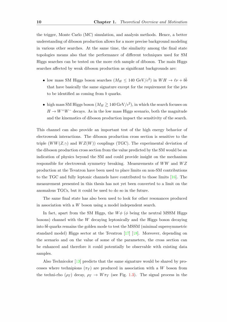
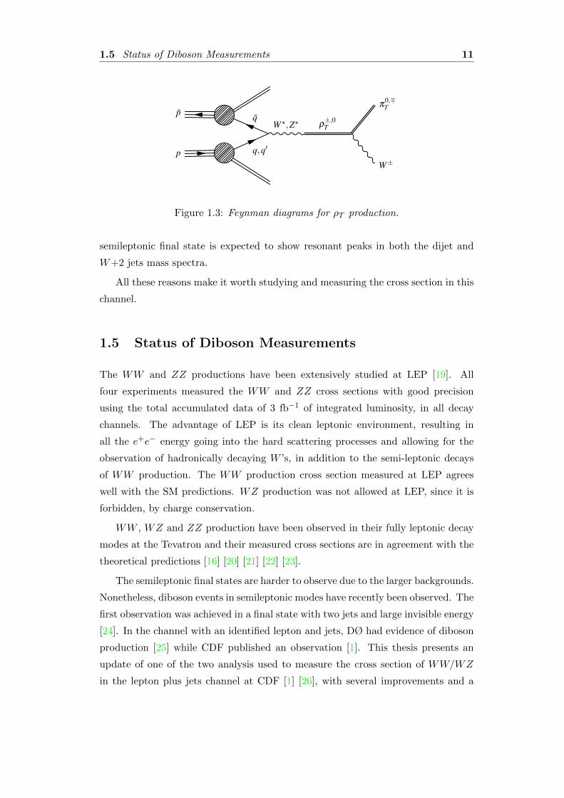
Also Technicolor [13] predicts that the same signature would be shared by pro-
cesses where technipions (πT ) are produced in association with a W boson from
the techni-rho (ρT ) decay, ρT → WπT (see Fig. 1.3). The signal process in the
1.5 Status of Diboson Measurements 11
q,q′
qW ⋆,Z⋆ ρ
±,0T
p
p
W±
π0,∓T
Figure 1.3: Feynman diagrams for ρT production.
semileptonic final state is expected to show resonant peaks in both the dijet and
W+2 jets mass spectra.
All these reasons make it worth studying and measuring the cross section in this
channel.
1.5 Status of Diboson Measurements
The WW and ZZ productions have been extensively studied at LEP [19]. All
four experiments measured the WW and ZZ cross sections with good precision
using the total accumulated data of 3 fb−1 of integrated luminosity, in all decay
channels. The advantage of LEP is its clean leptonic environment, resulting in
all the e+e− energy going into the hard scattering processes and allowing for the
observation of hadronically decaying W ’s, in addition to the semi-leptonic decays
of WW production. The WW production cross section measured at LEP agrees
well with the SM predictions. WZ production was not allowed at LEP, since it is
forbidden, by charge conservation.
WW , WZ and ZZ production have been observed in their fully leptonic decay
modes at the Tevatron and their measured cross sections are in agreement with the
theoretical predictions [16] [20] [21] [22] [23].
The semileptonic final states are harder to observe due to the larger backgrounds.
Nonetheless, diboson events in semileptonic modes have recently been observed. The
first observation was achieved in a final state with two jets and large invisible energy
[24]. In the channel with an identified lepton and jets, DØ had evidence of diboson
production [25] while CDF published an observation [1]. This thesis presents an
update of one of the two analysis used to measure the cross section of WW/WZ
in the lepton plus jets channel at CDF [1] [26], with several improvements and a
12 Chapter 1. Theoretical Overview and Motivation
Process Experiment L (fb−1) Measured σ (pb) Theory σ (pb)
WW → `ν`ν CDF [21] 3.6 12.1± 0.9(stat.)+1.0−1.4(syst.) 11.66± 0.70
DØ [20] 1 11.5± 2.2(stat.+sys.)
ZZ → ```` CDF [23] 6 1.7+1.2−0.7(stat.)± 0.2(syst.) 1.4± 0.1
WZ → ```ν CDF [23] 6 4.1± 0.6(stat.)± 0.4(syst.) 3.46± 0.30
DØ [22] 1 2.7+1.7−1.3(stat.+sys.)
WW/WZ/ZZ → νν + jets CDF [24] 3.5 18.6± 2.8(stat.)± 2.6(syst.) 16.8± 0.50
WW/WZ → `ν + jets DØ [25] 1.0 20.2± 4.5(stat.+sys.) 15.9± 0.9
CDF[2] 4.3 18.1± 3.3(stat.)± 2.5(syst.)
CDF[26] 4.6 16.5+3.3−3.0(stat.+sys.)
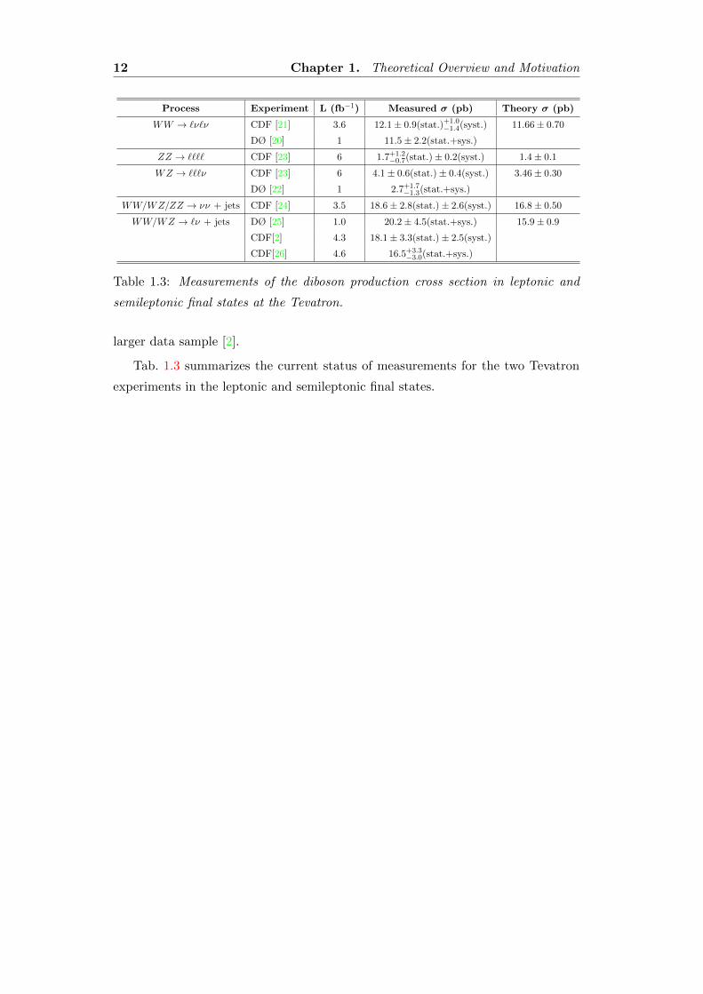
Table 1.3: Measurements of the diboson production cross section in leptonic and
semileptonic final states at the Tevatron.
larger data sample [2].
Tab. 1.3 summarizes the current status of measurements for the two Tevatron
experiments in the leptonic and semileptonic final states.
Chapter 2
Experimental Apparatus
The measurement described in this thesis is based on a data sample collected by the
CDFII detector during Run II operations at the Fermilab’s Tevatron Collider. This
chapter provides a general description of the experimental apparatus, both collider
and detector, focusing on the more relevant elements for this analysis.
2.1 The Tevatron Collider
The Tevatron [27] located at the Fermi National Accelerator Laboratory (Fermilab)
in Batavia (Illinois, USA) is a proton-antiproton (pp) collider with a center-of-mass
energy of 1.96 TeV.
The Tevatron started operating in 1975 as the first superconducting synchrotron,
the first pp collisions occurred in 1985 and since the year 2002 it operates only in
the collider mode. The upgraded machine collides 36 × 36 bunches every 396 ns.
As shown in Fig. 2.1, the Tevatron complex has five major accelerators and storage
rings used in successive steps, to produce, store and accelerate the particles up to
980 GeV.
2.1.1 Proton Production
The acceleration cycle starts with the production of protons from ionized hydrogen
atoms, H−, which are accelerated to 750 KeV of kinetic energy by a Cockroft-
Walton electrostatic accelerator.
Pre-accelerated H− ions are then injected into the LINAC where they are ac-
celerated up to 400 MeV by passing through a 150 m long chain of radio-frequency
13
14 Chapter 2. Experimental Apparatus
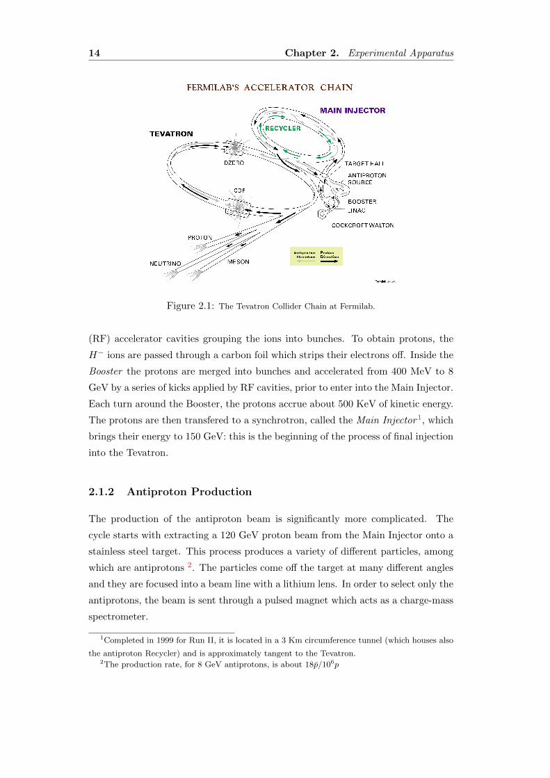
Figure 2.1: The Tevatron Collider Chain at Fermilab.
(RF) accelerator cavities grouping the ions into bunches. To obtain protons, the
H− ions are passed through a carbon foil which strips their electrons off. Inside the
Booster the protons are merged into bunches and accelerated from 400 MeV to 8
GeV by a series of kicks applied by RF cavities, prior to enter into the Main Injector.
Each turn around the Booster, the protons accrue about 500 KeV of kinetic energy.
The protons are then transfered to a synchrotron, called the Main Injector1, which
brings their energy to 150 GeV: this is the beginning of the process of final injection
into the Tevatron.
2.1.2 Antiproton Production
The production of the antiproton beam is significantly more complicated. The
cycle starts with extracting a 120 GeV proton beam from the Main Injector onto a
stainless steel target. This process produces a variety of different particles, among
which are antiprotons 2. The particles come off the target at many different angles
and they are focused into a beam line with a lithium lens. In order to select only the
antiprotons, the beam is sent through a pulsed magnet which acts as a charge-mass
spectrometer.
1Completed in 1999 for Run II, it is located in a 3 Km circumference tunnel (which houses also
the antiproton Recycler) and is approximately tangent to the Tevatron.2The production rate, for 8 GeV antiprotons, is about 18p/106p
2.1 The Tevatron Collider 15
The emerging antiprotons, having a bunch structure similar to that of the inci-
dent protons and a large energy spread, are stored in a Debuncher, a storage ring
where their momentum spread is reduced via stochastic cooling stations. Here, the
bunch structure is destroyed resulting in a continuous beam of antiprotons. At the
end of the process the monochromatic antiprotons are stored in the Accumulator,
which is a triangle-shaped storage ring where they are further cooled and stored
until the cycles of the Debuncher are completed.
After the accumulator has collected a sufficient amount of antiprotons (∼ 6 ×10¹¹), they are transferred to the Recycler3 which is an 8 GeV storage ring made of
permanent magnets and further cooled using stochastic cooling and accumulated.
When a current sufficient to create 36 bunches with the required density is available,
the p are injected into the Main Injector where they are accelerated to 150 GeV.
2.1.3 Tevatron
The Tevatron is a large synchrotron, 1 Km in radius, that accelerates particles from
150 GeV to 980 GeV. It keeps both protons and antiprotons in the same beampipe,
revolving in opposite directions. Electrostatic separators produce a strong electric
field that keeps the two beams from touching except at the collision point. The beam
is steered by 774 superconducting dipole magnets and 240 quadrupole magnets with
a maximum magnetic field of 4.2 T. They are cooled by liquid helium to 4.2 K, at
which point the niobium-titanium alloy in the magnets becomes superconducting.
The process of injecting particles into the machine, accelerating them, and initi-
ating collisions, referred to as a “shot”, starts with injection of protons, one bunch
at a time, at 150 GeV from the Main Injector. The antiprotons are injected three
bunches at a time from the Recycler through the Main Injector. RF cavities accel-
erate the beams to 980 GeV, and then some electrostatic separators switch polarity
to cause the beams to collide at two points. Each interaction point lies at the heart
of a particle detector: one named DØ (for the technical name of its position in
the Tevatron ring) and the other named the Collider Detector at Fermilab (CDF).
Stable running conditions and data-taking by the experiments are reached after
beams are scraped with remotely-operated collimators to remove the beam halo.
A continuous period of collider operation using the same collection of protons and
3Antiproton availability is the most limiting factor at Tevatron for attaining high luminosi-
ties: keeping a large stash of antiprotons inside the Recycler has been one of the most significant
engineering challenges and the excellent performance of the Recycler is an achievement of prime
importance for the good operation of the accelerator
16 Chapter 2. Experimental Apparatus
Parameter Run II value
number of bunches (Nb) 36
revolution frequency [MHz] (fbc) 1.7
bunch rms [m] σl 0.37
bunch spacing [ns] 396
protons/bunch (Np) 2.7× 10¹¹
antiprotons/bunch (Np) 3.0× 10¹⁰
total antiprotons 1.1× 10¹²
β∗ [cm] 35
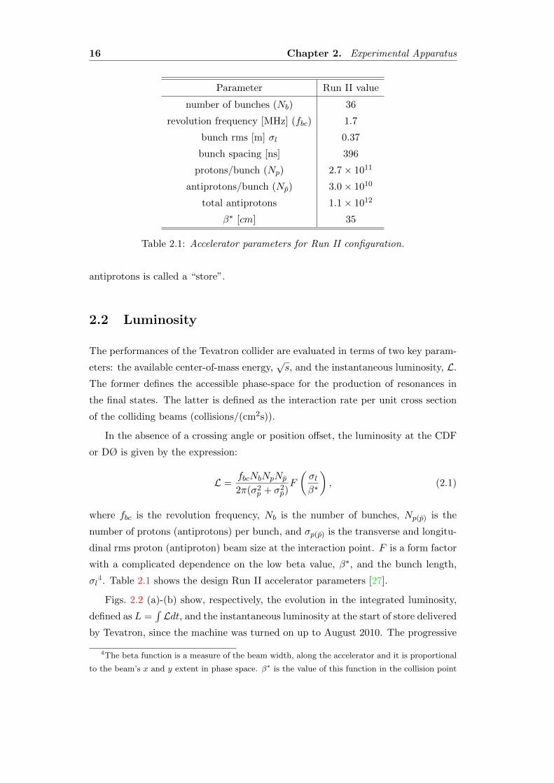
Table 2.1: Accelerator parameters for Run II configuration.
antiprotons is called a “store”.
2.2 Luminosity
The performances of the Tevatron collider are evaluated in terms of two key param-
eters: the available center-of-mass energy,√s, and the instantaneous luminosity, L.
The former defines the accessible phase-space for the production of resonances in
the final states. The latter is defined as the interaction rate per unit cross section
of the colliding beams (collisions/(cm2s)).
In the absence of a crossing angle or position offset, the luminosity at the CDF
or DØ is given by the expression:
L =fbcNbNpNp
2π(σ2p + σ2
p)F
(σlβ∗
), (2.1)
where fbc is the revolution frequency, Nb is the number of bunches, Np(p) is the
number of protons (antiprotons) per bunch, and σp(p) is the transverse and longitu-
dinal rms proton (antiproton) beam size at the interaction point. F is a form factor
with a complicated dependence on the low beta value, β∗, and the bunch length,
σl4. Table 2.1 shows the design Run II accelerator parameters [27].
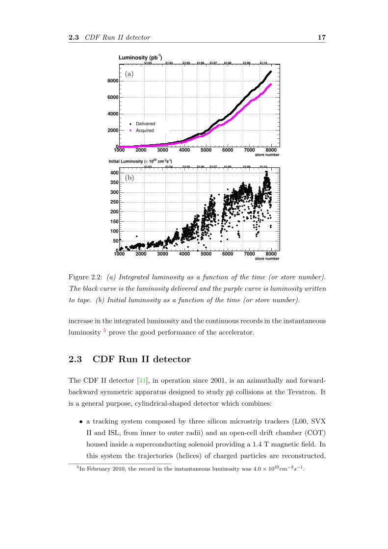
Figs. 2.2 (a)-(b) show, respectively, the evolution in the integrated luminosity,
defined as L =∫Ldt, and the instantaneous luminosity at the start of store delivered
by Tevatron, since the machine was turned on up to August 2010. The progressive
4The beta function is a measure of the beam width, along the accelerator and it is proportional
to the beam’s x and y extent in phase space. β∗ is the value of this function in the collision point
2.3 CDF Run II detector 17
store number1000 2000 3000 4000 5000 6000 7000 80000
2000
4000
6000
8000
01/1001/0901/0801/0701/0601/0501/0401/03
Delivered
Acquired
)-1
Luminosity (pb
(a)
store number1000 2000 3000 4000 5000 6000 7000 80000
50
100
150
200
250
300
350
400
01/1001/0901/0801/0701/0601/0501/0401/03
)-1s-2 cm30
10×Initial Luminosity (
(b)
Figure 2.2: (a) Integrated luminosity as a function of the time (or store number).
The black curve is the luminosity delivered and the purple curve is luminosity written
to tape. (b) Initial luminosity as a function of the time (or store number).
increase in the integrated luminosity and the continuous records in the instantaneous
luminosity 5 prove the good performance of the accelerator.
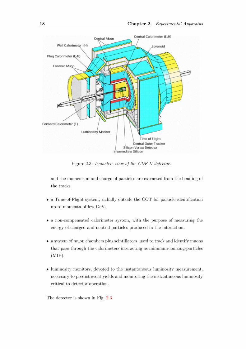
2.3 CDF Run II detector
The CDF II detector [41], in operation since 2001, is an azimuthally and forward-
backward symmetric apparatus designed to study pp collisions at the Tevatron. It
is a general purpose, cylindrical-shaped detector which combines:
• a tracking system composed by three silicon microstrip trackers (L00, SVX
II and ISL, from inner to outer radii) and an open-cell drift chamber (COT)
housed inside a superconducting solenoid providing a 1.4 T magnetic field. In
this system the trajectories (helices) of charged particles are reconstructed,
5In February 2010, the record in the instantaneous luminosity was 4.0 × 1032cm−2s−1.
18 Chapter 2. Experimental Apparatus
Figure 2.3: Isometric view of the CDF II detector.
and the momentum and charge of particles are extracted from the bending of
the tracks.
• a Time-of-Flight system, radially outside the COT for particle identification
up to momenta of few GeV.
• a non-compensated calorimeter system, with the purpose of measuring the
energy of charged and neutral particles produced in the interaction.
• a system of muon chambers plus scintillators, used to track and identify muons
that pass through the calorimeters interacting as minimum-ionizing-particles
(MIP).
• luminosity monitors, devoted to the instantaneous luminosity measurement,
necessary to predict event yields and monitoring the instantaneous luminosity
critical to detector operation.
The detector is shown in Fig. 2.3.
2.3 CDF Run II detector 19
2.3.1 Coordinate System and Useful Variables
The CDF detector is approximately cylindrically symmetric around the beam axis.
Its geometry can be described in cartesian as well as in cylindrical coordinates.
The left-handed cartesian system is centered on the nominal interaction point
with the z axis laying in the direction of the proton beam and the x axis on the
Tevatron plane pointing radially outside.
The cylindrical coordinates are the azimuthal angle, φ, and the polar angle, θ,:
φ = tan−1 y
xθ = tan−1
√x2 + y2
z
A momentum-dependent particle coordinate named rapidity is also commonly used.
The rapidity is defined as
Y =1
2lnE + pzE − pz
,
where E is the energy and pz is the z component of the momentum of the particle. It
is used instead of the polar angle θ because it is Lorentz invariant. In the relativistic
limit, or when the mass of the particle is ignored, rapidity becomes dependent only
upon the production angle of the particle with respect to the beam axis. This
approximation is called pseudorapidity η and is defined by
η = − ln(
tanθ
2
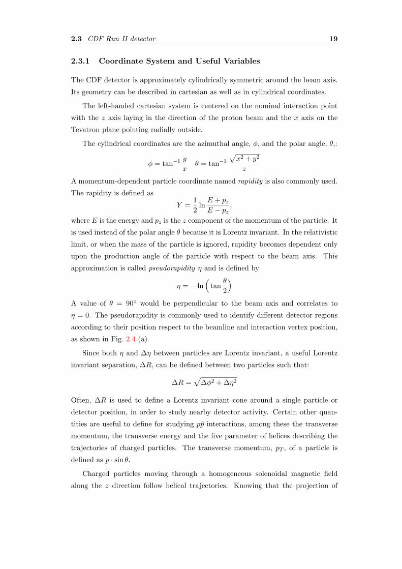
)A value of θ = 90◦ would be perpendicular to the beam axis and correlates to
η = 0. The pseudorapidity is commonly used to identify different detector regions
according to their position respect to the beamline and interaction vertex position,
as shown in Fig. 2.4 (a).
Since both η and ∆η between particles are Lorentz invariant, a useful Lorentz
invariant separation, ∆R, can be defined between two particles such that:
∆R =√
∆φ2 + ∆η2
Often, ∆R is used to define a Lorentz invariant cone around a single particle or
detector position, in order to study nearby detector activity. Certain other quan-
tities are useful to define for studying pp interactions, among these the transverse
momentum, the transverse energy and the five parameter of helices describing the
trajectories of charged particles. The transverse momentum, pT , of a particle is
defined as p · sin θ.Charged particles moving through a homogeneous solenoidal magnetic field
along the z direction follow helical trajectories. Knowing that the projection of
20 Chapter 2. Experimental Apparatus
(a) (b)
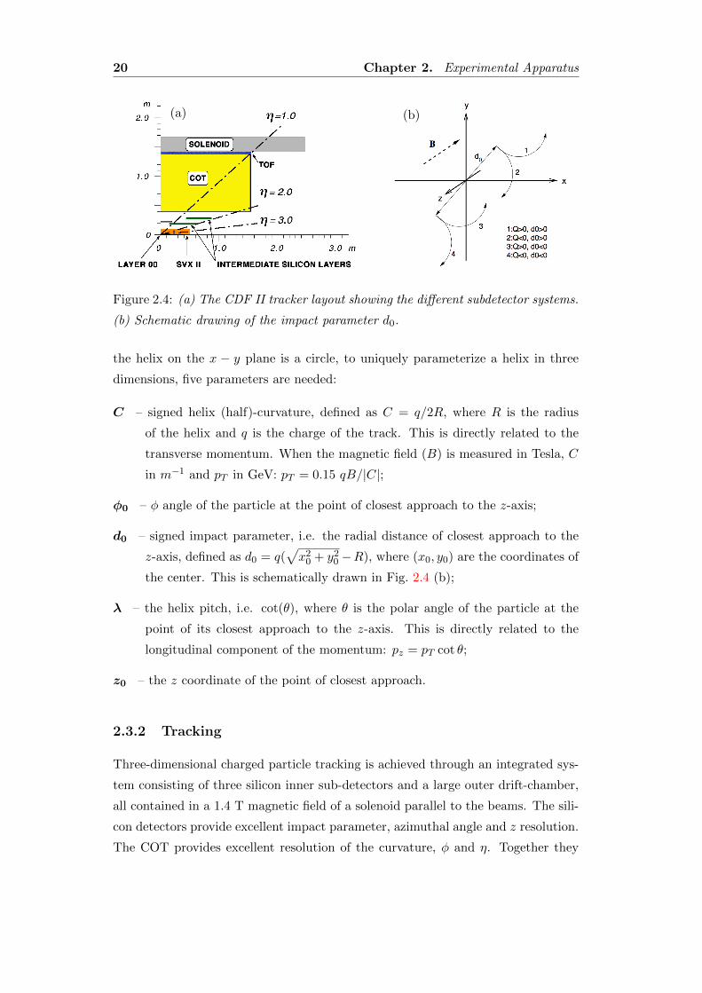
Figure 2.4: (a) The CDF II tracker layout showing the different subdetector systems.
(b) Schematic drawing of the impact parameter d0.
the helix on the x − y plane is a circle, to uniquely parameterize a helix in three
dimensions, five parameters are needed:
C – signed helix (half)-curvature, defined as C = q/2R, where R is the radius
of the helix and q is the charge of the track. This is directly related to the
transverse momentum. When the magnetic field (B) is measured in Tesla, C
in m−1 and pT in GeV: pT = 0.15 qB/|C|;
φ0 – φ angle of the particle at the point of closest approach to the z-axis;
d0 – signed impact parameter, i.e. the radial distance of closest approach to the
z-axis, defined as d0 = q(√x2
0 + y20 −R), where (x0, y0) are the coordinates of
the center. This is schematically drawn in Fig. 2.4 (b);
λ – the helix pitch, i.e. cot(θ), where θ is the polar angle of the particle at the
point of its closest approach to the z-axis. This is directly related to the
longitudinal component of the momentum: pz = pT cot θ;
z0 – the z coordinate of the point of closest approach.
2.3.2 Tracking
Three-dimensional charged particle tracking is achieved through an integrated sys-
tem consisting of three silicon inner sub-detectors and a large outer drift-chamber,
all contained in a 1.4 T magnetic field of a solenoid parallel to the beams. The sili-
con detectors provide excellent impact parameter, azimuthal angle and z resolution.
The COT provides excellent resolution of the curvature, φ and η. Together they
2.3 CDF Run II detector 21
provide a very accurate measurements of the helical paths of charged particles. We
will describe this system starting from the devices closest to the beam and moving
outwards (see Fig. 2.4 (a)).
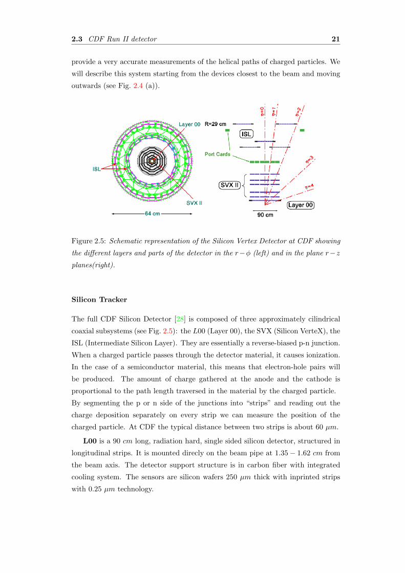
Figure 2.5: Schematic representation of the Silicon Vertex Detector at CDF showing
the different layers and parts of the detector in the r−φ (left) and in the plane r−zplanes(right).
Silicon Tracker
The full CDF Silicon Detector [28] is composed of three approximately cilindrical
coaxial subsystems (see Fig. 2.5): the L00 (Layer 00), the SVX (Silicon VerteX), the
ISL (Intermediate Silicon Layer). They are essentially a reverse-biased p-n junction.
When a charged particle passes through the detector material, it causes ionization.
In the case of a semiconductor material, this means that electron-hole pairs will
be produced. The amount of charge gathered at the anode and the cathode is
proportional to the path length traversed in the material by the charged particle.
By segmenting the p or n side of the junctions into “strips” and reading out the
charge deposition separately on every strip we can measure the position of the
charged particle. At CDF the typical distance between two strips is about 60 µm.
L00 is a 90 cm long, radiation hard, single sided silicon detector, structured in
longitudinal strips. It is mounted direcly on the beam pipe at 1.35− 1.62 cm from
the beam axis. The detector support structure is in carbon fiber with integrated
cooling system. The sensors are silicon wafers 250 µm thick with inprinted strips
with 0.25 µm technology.
22 Chapter 2. Experimental Apparatus
Being so close to the beam, L00 allows to reach a resolution of ∼ 25/30 µm
on the impact parameter of tracks of moderate pT , providing a powerful help to
identify long-lived hadrons containing a b quark.
SVX is composed of a set of three cylindrical barrels [29]. Barrels are radially
organized in five layers of double-sided silicon wafers extending from 2.5 cm to
10.7 cm. Three of those layers provide ϕ measurement on one side and 90o z on the
other, while the other two provide ϕ measurement in one side and a z measurement
by small angle 1.2o stereo on the other.
The SVX detector has ∼ 90 cm of total active length, which corresponds to
about 3σ of the gaussian longitudinal spread of the interaction point, and provides
pseudorapidity coverage in the |η| < 2 region. The resolution on the single hit is 12
µm.
The ISL consists of 5 layers of double sided silicon wafers: four are assembled
in two telescopes at 22 cm and 29 cm radial distance from the beamline covering
1 < |η| < 2. One is central at r = 22 cm, covering |η| < 1. The two ISL layers are
important to help tracking in a region where the COT coverage is incomplete.
All the silicon detectors are used in the offline track reconstruction algorithms,
while SVX plays a crucial role in the both for the online reconstruction and for the
B hadrons trigger. CDF employs an innovative processor SVT [30] for the online
track reconstruction in the silicon detector. The SVT was upgraded [31] to cope
with the higher Tevatron luminosity. The SVT reconstruction is precise enough
for online identification of secondary vertexes of B hadron decays (displaced by the
primary interaction point).
COT
Surrounding the silicon detector is the Central Outer Tracker (COT) [32], the anchor
of the CDF Run II tracking system. It is a 3.1 m long cylindrical drift chamber
that covers the radial range from 40 to 137 cm (|η| < 1). The COT contains 96
sense wire layers, which are radially grouped into eight “superlayers”, as inferred
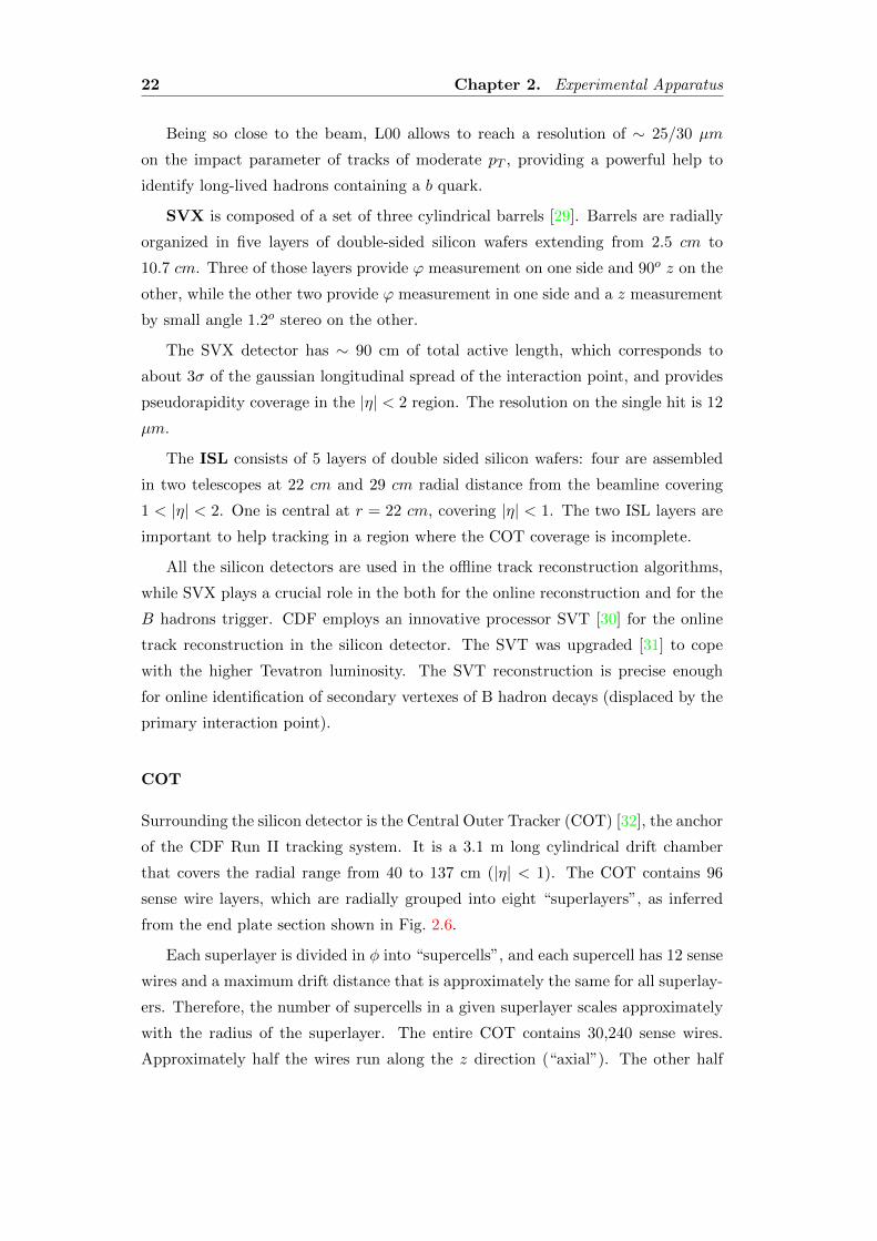
from the end plate section shown in Fig. 2.6.
Each superlayer is divided in φ into “supercells”, and each supercell has 12 sense
wires and a maximum drift distance that is approximately the same for all superlay-
ers. Therefore, the number of supercells in a given superlayer scales approximately
with the radius of the superlayer. The entire COT contains 30,240 sense wires.
Approximately half the wires run along the z direction (“axial”). The other half
2.3 CDF Run II detector 23
(a)
SL252 54 56 58 60 62 64 66
R
Potential wires
Sense wires
Shaper wires
Gold on Mylar (Field Panel)
R (cm)
(b)
Figure 2.6: (a) Layout of wire planes on a COT endplate. (b) Layout of wires in a
COT supercell.
are strung at a small angle (2◦) with respect to the z direction (“stereo”). The com-
bination of the axial and stereo information allows us to measure the z positions.
Particles originated from the interaction point, which have |η| < 1, pass through all
8 superlayers of the COT.
The supercell layout, shown in figure 2.6 for superlayer 2, consists of a wire
plane containing sense and potential wires, for field shaping and a field (or cathode)
sheet on either side. Both the sense and potential wires are 40 µm diameter gold
plated tungsten. The field sheet is 6.35 µm thick Mylar with vapor-deposited gold
on both sides. Each field sheet is shared with the neighboring supercell.
The COT is filled with an Argon-Ethane gas mixture and Isopropyl alcohol
(49.5:49.5:1). The mixture is chosen to have a constant drift velocity, approximately
50 µm/ns, across the cell width and the small content of isopropyl alcohol is intended
to reduce the aging and build up on the wires. When a charged particle passes
through, the gas is ionized. Electrons drift toward the sense wires. Due to the
magnetic field that the COT is immersed in, electrons drift at a Lorentz angle of
35◦. The supercell is tilted by 35◦ with respect to the radial direction to compensate
for this effect. The hit resolution in r − φ is about 140 µm and the transverse
momentum resolution of the tracks in the COT chamber depends on the pT and is
measured to be σ(pT )/p2T ≈ 0.15% (GeV/c)−1 for tracks with pT > 2 GeV/c [33].
24 Chapter 2. Experimental Apparatus
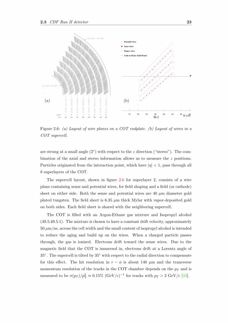
Figure 2.7: Elevation view of 1/4 of the CDF detector showering the components of
the CDF calorimeter: CEM, CHA, WHA, PEM and PHA.
In addition to the measurement of the charged particle momenta, the COT is
used to identify particles based on dE/dx measurements.
2.3.3 Time of Flight
Just outside the tracking system, see Fig. 2.4 (a), CDF II has a Time of Flight
(TOF) detector [34]. It is a barrel of scintillator almost 3 m long located at 140 cm
from the beam line with a total of 216 bars, each covering 1.7◦ in φ and pseudo-
rapidity range |η| < 1. Particle identification is achieved by measuring the time of
arrival of a charged particle at the scintillators with respect to the collision time.
Thus, combining the measured time-of-flight, the momentum and the path length,
measured by the tracking system, the mass of the particle can be estimated. The
resolution in the time-of-flight measurement is ≈ 100 ps and it provides at least two
standard deviation separation between K± and π± for momenta p < 1.6 GeV/c.
2.3.4 Calorimeter System
Surrounding the CDF tracking volume, outside of the solenoid coil, there is the
calorimeter system. The different calorimeters that compose the system are scintillator-
based detectors and segmented in projective towers (or wedges), in η×φ space, that
point to the interaction region. The total coverage of the system is 2π in φ and
about |η| < 3.64 units in pseudorapidity.
The calorimeter system is divided in two regions: central and plug. The central
2.3 CDF Run II detector 25
calorimeter covers the region |η| < 1.1 and is split into two halves at |η| = 0. The
forward plug calorimeters cover the angular range corresponding to 1.1 < |η| < 3.64,
as it is shown in Fig. 2.7. Due to this structure two “gap” regions are found at |η| = 0
and |η| ∼ 1.1.
Central Calorimeters
The central calorimeters consist of 478 towers, each one is 15◦ in azimuth by
about 0.11 in pseudorapidity. Each wedge consists of an electromagnetic component
backed by a hadronic section. The light from each tower is collected and shifted by
sheets of acrylic plastic placed on the azimuthal tower boundaries, and guided to
two phototubes per tower.
In the central electromagnetic calorimeter (CEM) [35], there are 31 layers of
polystyrene scintillator interleayed with layers of lead. The two outer towers (chim-
ney) in one wedge are missing to allow accessing the solenoid for check and repairs
if needed. The total material has a depth of 19 radiation lengths (X0) 6.
The central hadronic calorimeter CHA [36] surrounds the CEM covering the
region |η| < 0.9 and consists of 32 steel layers sampled each 2.5 cm by 1.0 cm-thick
acrylic scintillator. Filling a space between the CHA and the forward plug hadronic
calorimeter (PHA) two calorimeter rings cover the gap between CHA and PHA in
the region 0.7 < |η| < 1.3, the wall hadronic calorimeter (WHA), which continues
the tower structure of the CHA but with reduced sampling (each 5.0 cm). The total
thickness of the hadronic section is approximately constant and corresponds to 4.5
interaction lengths (λ0) 7.
The energy resolution for each section was measured in the test beam and, for
a perpendicular incident beam, it can be parameterized as
σ
E=
σ1√E⊕ σ2,
where the first term comes from sampling fluctuations and the photostatistics of
PMTs, and the second term comes from the non-uniform response of the calorimeter.
6The radiation length X0 describes the characteristic amount of matter transversed, for high-
energy electrons to lose all but 1/e of its energy by bremsstrahlung, which is equivalent to 79
of
the length of the mean free path for pair e+e− production of high-energy photons. The average
energy loss due to bremsstrahlung for an electron of energy E is related to the radiation length by(dEdx
)brems
= − EX0
.7An interaction length is the average distance a particle will travel before interacting with a
nucleus: λ = AρσNA
, where A is the atomic weight, ρ is the material density, σ is the cross section
and NA is the Avogadro’s number.
26 Chapter 2. Experimental Apparatus
In the CEM, the energy resolution for high energy electrons and photons is
σ(E)
E=
13.5%√ET⊕ 1.5%,
where ET = E sin θ being θ the beam incident angle.
Charge pions were used to obtain the energy resolution in the CHA and WHA
detectors that are
σ(E)
E=
50%√ET⊕ 3% and
σ(E)
E=
75%√ET⊕ 4%
respectively.
Plug Calorimeters
One of the major components upgraded for the Run II was the plug calorimeter [37].
The new plug calorimeters are built with the same technology as the central com-
ponents and replace the Run I gas calorimeters in the forward region. The η × φsegmentation depends on the tower pseudorapidity coverage. For towers in the
region |η| < 2.1, the segmentation is 7.5o in φ and from 0.1 to 0.16 in the pseudo-
rapidity direction. For more forward wedges, the segmentation changes to 15o in φ
and about 0.2 to 0.6 in η.
As in the central calorimeters, each wedge consists of an electromagnetic (PEM)
and a hadronic section (PHA). The PEM, with 23 layers composed of lead and
scintillator, has a total thickness of about 21 X0 . The PHA is a steel/scintillator
device with a depth of about 7 λ0. In both sections the scintillator tiles are read
out by WLS fibers embedded in the scintillator. The WLS fibers carry the light
out to PMTs tubes located on the back plane of each endplug. Unlike the central
calorimeters, each tower is only read out by one PMT.
The PEM energy resolution for high energy electrons and photons is:
σ
E=
16%√ET⊕ 1%.
The PHA energy resolution, for charged pions that do not interact in the elec-
tromagnetic component, is:
σ
E=
80%√ET⊕ 5%.
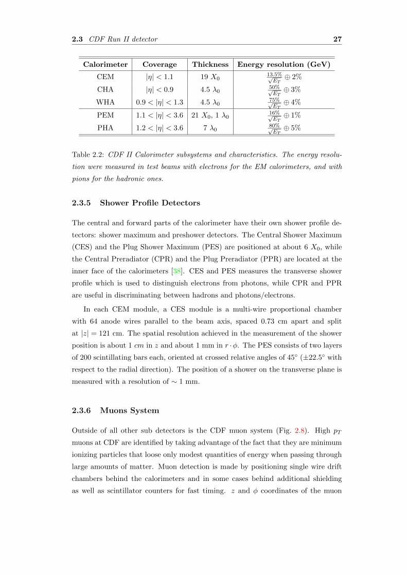
Table 2.2 summarizes the calorimeter subsystems and their characteristics.
2.3 CDF Run II detector 27
Calorimeter Coverage Thickness Energy resolution (GeV)
CEM |η| < 1.1 19 X013.5%√ET⊕ 2%
CHA |η| < 0.9 4.5 λ050%√ET⊕ 3%
WHA 0.9 < |η| < 1.3 4.5 λ075%√ET⊕ 4%
PEM 1.1 < |η| < 3.6 21 X0, 1 λ016%√ET⊕ 1%
PHA 1.2 < |η| < 3.6 7 λ080%√ET⊕ 5%
Table 2.2: CDF II Calorimeter subsystems and characteristics. The energy resolu-
tion were measured in test beams with electrons for the EM calorimeters, and with
pions for the hadronic ones.
2.3.5 Shower Profile Detectors
The central and forward parts of the calorimeter have their own shower profile de-
tectors: shower maximum and preshower detectors. The Central Shower Maximum
(CES) and the Plug Shower Maximum (PES) are positioned at about 6 X0, while
the Central Preradiator (CPR) and the Plug Preradiator (PPR) are located at the
inner face of the calorimeters [38]. CES and PES measures the transverse shower
profile which is used to distinguish electrons from photons, while CPR and PPR
are useful in discriminating between hadrons and photons/electrons.
In each CEM module, a CES module is a multi-wire proportional chamber
with 64 anode wires parallel to the beam axis, spaced 0.73 cm apart and split
at |z| = 121 cm. The spatial resolution achieved in the measurement of the shower
position is about 1 cm in z and about 1 mm in r ·φ. The PES consists of two layers
of 200 scintillating bars each, oriented at crossed relative angles of 45◦ (±22.5◦ with
respect to the radial direction). The position of a shower on the transverse plane is
measured with a resolution of ∼ 1 mm.
2.3.6 Muons System
Outside of all other sub detectors is the CDF muon system (Fig. 2.8). High pT
muons at CDF are identified by taking advantage of the fact that they are minimum
ionizing particles that loose only modest quantities of energy when passing through
large amounts of matter. Muon detection is made by positioning single wire drift
chambers behind the calorimeters and in some cases behind additional shielding
as well as scintillator counters for fast timing. z and φ coordinates of the muon
28 Chapter 2. Experimental Apparatus
candidate are provided by the chambers while the scintillator detectors are used for
triggering and spurious signal rejection.
The muon system [39, 40] is divided into different subsystems: the Central
Muon Detector, CMU, the Central Muon Upgrade Detector, CMP, the Central
Muon Extension Detector, CMX and the Intermediate Muon Detector, IMU. The
coverage of the muon systems is almost complete in φ, except for some gaps, and
spans in polar angle up to |η| ∼ 1.5, see Fig. 2.8.
CMU
The Central Muon Chambers (CMU) [41] is a set of four layered drift chamber
sandwiches, housed on the back of wedges inside the central calorimeter shells cov-
ering the region |η| < 0.6. It is cylindrical in geometry with a radius of 350 cm,
arranged into 12.6◦ wedges. Each wedge contains three modules (stacks) with four
layers of four rectangular drift cells. The cell are 266 cm x 2.68 cm x 6.35 cm wide
and they have 50 µm sense wire at the center of the cell, parallel to the z direction.
The system is filled with Argone-Ethane gas miixture and alcohol like the COT.
CMP
The Central Muon uPgrade (CMP) consists of a 4-layer sandwich of wire chambers
operated in proportional mode covering most of the |η| < 0.6 region where it overlaps
with CMU (see Fig. 2.8). It is located outside an additional layer of 60 cm thick
steel partially used for the magnetic field return, providing the needed shielding to
absorb particles, other than muons, leaking the calorimeter. Unlike mostly of the
CDF components, this subdetector is not cylinrically-shaped but box-like, because
CMP uses the magnet return yoke steel as an absorber, along with some additional
pieces of steel to fill gaps in the yoke. On the outer surface of CMP a scintillator
layer, the Central Scintillator Upgrade (CSP), measures the muon traversal time.
The system CMU/CMP, which is called CMUP, detects muons having a minimum
energy of ∼ 1.4 GeV .
CMX
The muon extension CMX is a large system of drift chambers-scintillator sandwiches
arranged in two truncated conical arches detached from the main CDF detector to
cover the region 0.6 < |η| < 1.0. Due to main detector frame structure, some
2.3 CDF Run II detector 29
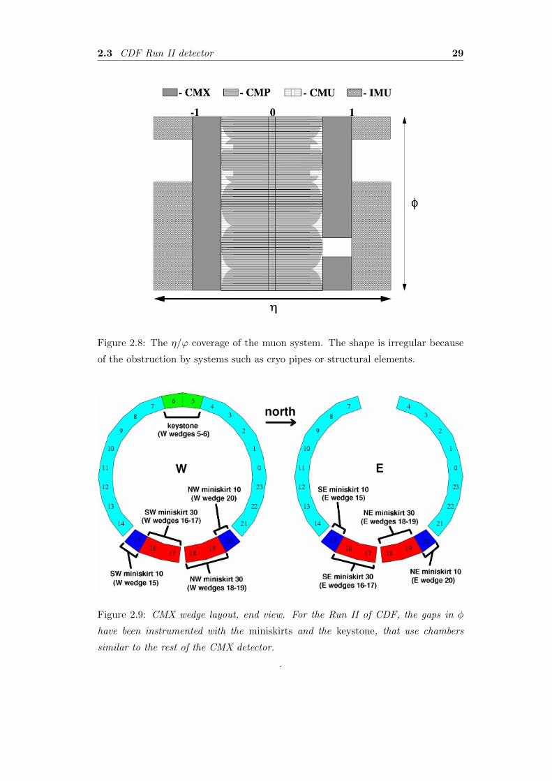
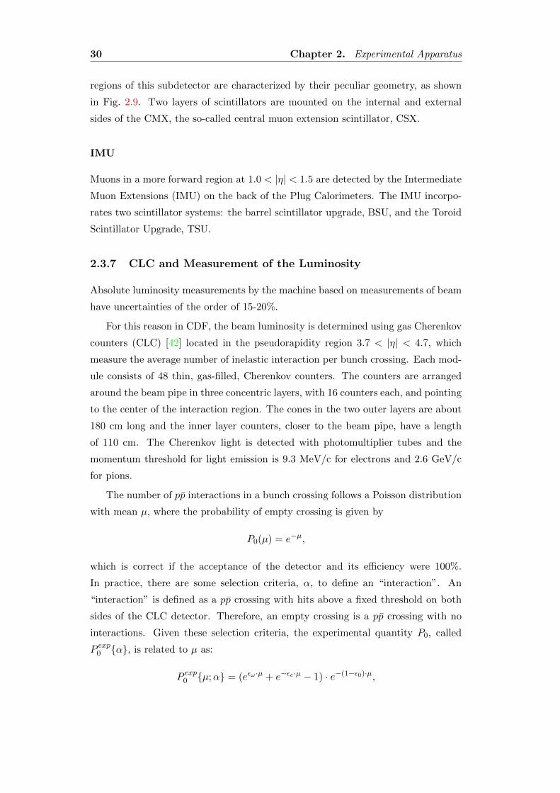
Figure 2.8: The η/ϕ coverage of the muon system. The shape is irregular because
of the obstruction by systems such as cryo pipes or structural elements.
Figure 2.9: CMX wedge layout, end view. For the Run II of CDF, the gaps in φ
have been instrumented with the miniskirts and the keystone, that use chambers
similar to the rest of the CMX detector.
.
30 Chapter 2. Experimental Apparatus
regions of this subdetector are characterized by their peculiar geometry, as shown
in Fig. 2.9. Two layers of scintillators are mounted on the internal and external
sides of the CMX, the so-called central muon extension scintillator, CSX.
IMU
Muons in a more forward region at 1.0 < |η| < 1.5 are detected by the Intermediate
Muon Extensions (IMU) on the back of the Plug Calorimeters. The IMU incorpo-
rates two scintillator systems: the barrel scintillator upgrade, BSU, and the Toroid
Scintillator Upgrade, TSU.
2.3.7 CLC and Measurement of the Luminosity
Absolute luminosity measurements by the machine based on measurements of beam
have uncertainties of the order of 15-20%.
For this reason in CDF, the beam luminosity is determined using gas Cherenkov
counters (CLC) [42] located in the pseudorapidity region 3.7 < |η| < 4.7, which
measure the average number of inelastic interaction per bunch crossing. Each mod-
ule consists of 48 thin, gas-filled, Cherenkov counters. The counters are arranged
around the beam pipe in three concentric layers, with 16 counters each, and pointing
to the center of the interaction region. The cones in the two outer layers are about
180 cm long and the inner layer counters, closer to the beam pipe, have a length
of 110 cm. The Cherenkov light is detected with photomultiplier tubes and the
momentum threshold for light emission is 9.3 MeV/c for electrons and 2.6 GeV/c
for pions.
The number of pp interactions in a bunch crossing follows a Poisson distribution
with mean µ, where the probability of empty crossing is given by
P0(µ) = e−µ,
which is correct if the acceptance of the detector and its efficiency were 100%.
In practice, there are some selection criteria, α, to define an “interaction”. An
“interaction” is defined as a pp crossing with hits above a fixed threshold on both
sides of the CLC detector. Therefore, an empty crossing is a pp crossing with no
interactions. Given these selection criteria, the experimental quantity P0, called
P exp0 {α}, is related to µ as:
P exp0 {µ;α} = (eεω ·µ + e−εe·µ − 1) · e−(1−ε0)·µ,
2.4 Trigger and Data Acquisition 31
where the acceptances ε0 and εω/e are, respectively, the probability to have no hits
in the combined east and west CLC modules and the probability to have at least
one hit exclusively in west/east CLC module. The evaluation of these parameters is
based on Monte Carlo simulations, and typical values are ε0=0.07 and εω/e = 0.12.
From the measurement of µ we can extract the luminosity. Since the CLC is not
sensitive at all to the elastic component of the pp scattering, the rate of inelastic pp
interactions is given by:
µ · fbc = σin · L,
where fbc is the bunch crossings frequency at Tevatron and σin is the inelastic pp
cross section. σin = 60.7±2.0 mb, is obtained by extrapolating the combined results
for the inelastic pp cross section of CDF at√s = 1.8 TeV and E811 measurements
at√s = 1.96 TeV[43].
Different sources of uncertainties have been taken into account to evaluate the
systematic uncertainties on the luminosity measurement [47]. The dominated con-
tributions are related to the detector simulation and the event generator used, and
have been evaluated to be about 3%. The total uncertainty in the CLC luminosity
measurements is 5.8%, which includes uncertainties on the measurement (4.2%) and
on the inelastic cross section value (4%).
2.4 Trigger and Data Acquisition
The average interaction rate at the Tevatron is 1.7 MHz for 36×36 bunches. In fact,
the actual interaction rate is higher because the bunches circulate in three trains of
12 bunches in each group spaced 396 ns, which leads to a crossing rate of 2.53 MHz.
The interaction rate is orders of magnitude higher than the maximum rate that
the data acquisition system can handle. Furthermore, the majority of collisions are
not of interest. This leads to implementation of a trigger system that preselects
events online and decides if the corresponding event information is written to tape
or discarded.
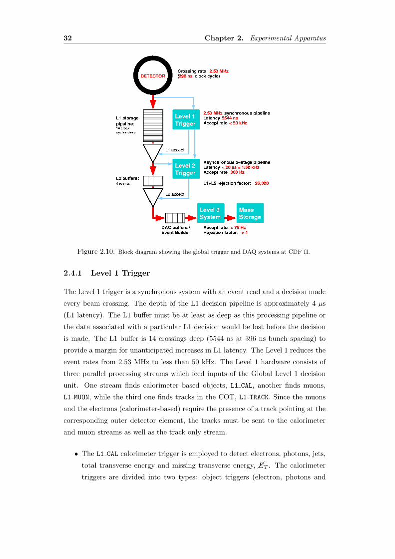
The CDF trigger system consists of three trigger levels, see Fig. 2.10. The first
two levels are hardware based and the third one is a processor farm. The decisions
taken by the system are based on increasingly more complex event information.
The two hardware levels are monitored and controlled by the Trigger Supervisor
Interface (TSI), which distributes signals from the different sections of the trigger
and DAQ system, a global clock and bunch crossing signal.
32 Chapter 2. Experimental Apparatus
Figure 2.10: Block diagram showing the global trigger and DAQ systems at CDF II.
2.4.1 Level 1 Trigger
The Level 1 trigger is a synchronous system with an event read and a decision made
every beam crossing. The depth of the L1 decision pipeline is approximately 4 µs
(L1 latency). The L1 buffer must be at least as deep as this processing pipeline or
the data associated with a particular L1 decision would be lost before the decision
is made. The L1 buffer is 14 crossings deep (5544 ns at 396 ns bunch spacing) to
provide a margin for unanticipated increases in L1 latency. The Level 1 reduces the
event rates from 2.53 MHz to less than 50 kHz. The Level 1 hardware consists of
three parallel processing streams which feed inputs of the Global Level 1 decision
unit. One stream finds calorimeter based objects, L1 CAL, another finds muons,
L1 MUON, while the third one finds tracks in the COT, L1 TRACK. Since the muons
and the electrons (calorimeter-based) require the presence of a track pointing at the
corresponding outer detector element, the tracks must be sent to the calorimeter
and muon streams as well as the track only stream.
• The L1 CAL calorimeter trigger is employed to detect electrons, photons, jets,
total transverse energy and missing transverse energy, ��ET . The calorimeter
triggers are divided into two types: object triggers (electron, photons and
2.4 Trigger and Data Acquisition 33
jets) and global triggers (∑ET and ��ET ). The calorimeter towers are summed
into trigger towers of 15o in φ and by approximately 0.2 in η. Therefore, the
calorimeter is divided in 24 x 24 towers in η×φ space. The object triggers are
formed by applying thresholds to individual calorimeter trigger towers, while
thresholds for the global triggers are applied after summing energies from all
towers.
• The L1 TRACK trigger is designed to detect tracks in the COT. An eXtremely
Fast Tracker (XFT) uses hits from 4 axial layers of the COT to find tracks
with a pT greater than some threshold (∼ 2 GeV/c). The resulting track list
is sent to the extrapolation box (XTRP) that distributes the tracks to the
Level 1 and Level 2 trigger subsystems.
• L1 MUON system uses muon primitives, generated from various muon detector
elements, and XFT tracks extrapolated to the muon chambers by the XTRP
to form muon trigger objects. For the scintillators of the muon system, the
primitives are derived from single hits or coincidences of hits. In the case of the
wire chambers, the primitives are obtained from patterns of hits on projective
wire with the requirement that the difference in the arrival times of signals be
less than a present threshold. This maximum allowed time difference imposes
a minimum pT requirement for hits from a single tracks.
Finally, the Global Level 1 makes the L1 trigger decision based on the objects of
interest found by the different Level 1 processes. Different sets of Level 1 conditions
are assigned to the L1 trigger bits. If these conditions are met, the bit is set to true.
All this information is later handled by the TSI and transfered to the other trigger
levels, and eventually, to tape. Finally, the Global Level 1 makes the L1 trigger
decision based on the quantity of each trigger object passed to it.
2.4.2 Level 2 Trigger
The Level 2 trigger is an asynchronous system which processes events that have
received a L1 accept in FIFO (First In, First Out) manner. It is structured as
a two stage pipeline with data buffering at the input of each stage. The first
stage is based on dedicated hardware processor which assembles information from
a particular section of the detector. The second stage consists of a programmable
processors operating on lists of objects generated by the first stage. Each of the L2
stages is expected to take approximately 10 µs giving a latency of approximately
34 Chapter 2. Experimental Apparatus
20 µs. The L2 buffers provide a storage of four events. After the Level 2, the event
rate is reduced to about 300 Hz.
In addition of the trigger primitives generated for L1, data for the L2 come from
the shower maximum strip chambers in the central calorimeter and the r×φ strips
of the SVX II. There are three hardware systems generating primitives at Level
2: Level 2 cluster finder (L2CAL), shower maximum strip chambers in the central
calorimeter (XCES) and the Silicon Vertex Trigger (SVT).
• The L2CAL hardware carries out the hardware cluster finder functions. It re-
ceives trigger tower energies from the L1 CAL and applies seed and ‘shoulder”
thresholds for cluster finding. It is basically designed for jet triggers.
• The shower maximum detector provides a much better spacial resolution than
a calorimeter wedge. The XCES boards perform sum of the energy on groups
of four adjacent CES wires and compare them to a threshold (around 4 GeV).
This information is matched to XFT tracks to generate a Level 2 trigger. This
trigger hardware provides a significant reduction in combinatorial background
for electrons and photons.
• Silicon Vertex Tracker [30] uses hits from the r × φ strips of the SVX II
and tracks from the XFT to find tracks in SVX II. SVT improves on the
XFT resolution for φ and pT and adds a measurement of the track impact
parameter d0. Hereby the efficiency and resolution are comparable to those
of the offline track reconstruction. The SVT enables triggering on displaced
tracks, that have a large impact parameter d0.
The Level 2 trigger has worked well for Run II at low luminosity. However, as
the Tevatron instantaneous luminosity increases, the limitation due to the simple
algorithms used, starts to become clear. For this reason, two major trigger upgrades
were implemented during 2007, the Level 2 XFT stereo upgrade and the Level 2
calorimer upgrade [48].
The upgrade makes use of the full calorimeter trigger tower information directly
available to the Level 2 decision CPU. The upgraded system allows more sophisti-
cated algorithms to be implemented in software; both Level 2 jets and ��ET can be
made nearly equivalent to offline quality, thus significantly improving the purity as
well as the efficiency of the jet and ��ET related triggers. The jet triggers are im-
proved by using a cone algorithm in the Level 2 CPU for jet cluster finding. The jet
algorithm is similar to JetClu (which is used to reconstruct Level 3 and offline jets)

2.4 Trigger and Data Acquisition 35
except that the clustering is done in a single iteration, in order to save processing
time.
2.4.3 Level 3 Trigger
When an event is accepted by the Level 2 trigger, its data become available for
readout distributed over a couple of hundred of VME Readout Buffers (VRBs). The
event has to be assembled from pieces of data from the L2 system into complete
events, this is the purpose of the Event Builder. It is divided into 16 sub-farms,
each consisting of 12-16 processor nodes. Once the event is built, it is sent to one
place in the Level 3 farm. The Level 3 trigger reconstructs the event following given
algorithms. These algorithms take advantage of the full detector information and
improved resolution not available to the lower trigger levels. This includes a full
3-dimensional track reconstruction and tight matching of tracks to calorimeter and
muon-system information. Events that satisfy the Level 3 trigger requirements are
then transferred onward to the Consumer Server/Data Logger (CSL) system for
storage first on disk and later on tape. The average processing time per event in
Level 3 is on the order of one second. The Level 3 leads to a further reduction in
the output rate, a roughly 50 Hz.
A set of requirements that an event has to fulfill at Level 1, Level 2 and Level 3
constitutes a trigger path. The CDF II trigger system implements about 150 trigger
paths. A complete description of the different datasets at CDF Run II can be found
in [49].
The trigger system described above is able to use the information of quite any
detector subsystem. Combining all the measurements of the various subsystems it
is possible to efficiently record, at the same time, events characterized by different
signatures. Indeed the data collected by CDF II can be used to study the properties
of the top quark, weak bosons, as well as the decays of b and c hadrons and more
generally SM processes, or to search evidence of physics beyond the SM.
The trigger path used in this analysis require a central high pT electron or muon
and will be briefly described in Sec. 4.3.

36 Chapter 2. Experimental Apparatus

Chapter 3
Objects Identification and
Event Reconstruction
All the quantities measured by the CDF sub-detectors have to be processed in
order to reconstruct the observables needed to study the physical products of the
pp collision. This chapter briefly explains how from “raw” data we first reconstruct
high level detector objects (such as tracks, vertices and calorimeter clusters) and
how these are then combined to identify the physical objects (electrons, muons,
neutrinos and jets) of interest for the analysis described in this thesis.
3.1 High Level Detector Objects
The detector outputs are primarily used to reconstruct high level objects, which
include tracks, trajectories of charged particles identified as sequences of “hits”
in the tracking detectors, and calorimeter clusters, collections of towers in which
energy from particles is deposited. Multiple-track reconstruction allows to identify
the vertices where either the pp interaction (primary vertex) or the decay of a long-
lived particle (secondary or displaced vertex) took place.
3.1.1 Tracking
As explained in the previous chapter, charged particles leave small charge depo-
sitions as they pass through the alternative layers of the tracking system. Using
these depositions, pattern recognition algorithms can reconstruct the particle origi-
nal trajectory measuring the five parameters of the helix (see Sect. 2.3.1) that best
37
38 Chapter 3. Objects Identification and Event Reconstruction
match to the observed hits.
CDF employs several algorithms for tracks reconstruction depending on which
component of the detector a particle travels through. The principal one is the
Outside-In (OI) [50]. This algorithm, exploiting the informations from both the
central drift chamber and the silicon detectors, is used to track the particles in
the central region (|η| < 1). It first reconstructs tracks in the COT and then
extrapolates them inwards toward the beam.
The first step of pattern recognition in the COT looks for circular paths1 in the
axial superlayers. Cells in the axial superlayers are searched for sets of 4 or more hits
that can be fit to a straight line. These sets are called “segments”. Once segments
are found, there are two approaches to track finding [51] (“segment linking” and
“histogram linking” algorithms). One approach is to link together the segments
which are consistent with lying tangent to a common circle. The other approach is
to constrain its circular fit to the “beamline” (see Sec.3.1.2). Once a circular path
is found in the r − φ plane, segments and hits in the stereo superlayer are added
depending on their proximity to the circular fit. This results in a three-dimensional
track fit. Typically, if one algorithm fails to reconstruct a track, the other algorithm
will not. This results in a high track reconstruction efficiency in the COT for tracks
which pass through all 8 superlayers (97% for tracks with pT > 10 GeV/c)2.
Once a track is reconstructed in the COT, it is extrapolated inward to the
silicon system. Based on the estimated errors on the track parameters, a three
dimensional “road” is formed around the extrapolated track. Starting from the
outermost layer, and working inwards, silicon hits found inside the road are added
to the track. As hits get added, the road gets narrowed according to the knowledge
of the updated track parameters and their covariance matrix. Reducing the width
of the road reduces the chance of adding a wrong hit to the track, and also reduces
the computation time. In the first pass of this algorithm, axial hits are added. In
the second pass, hits with stereo information are added to the track. At the end,
the track combination with the highest number of hits and lowest χ2/ndf for the
five parameters helix fit is kept.
Due to the limited COT coverage and the strict hits requirement (at least four
of eight superlayers), tracking in the forward region requires different algorithms
1The helical track, when projected onto the r − φ plane, is a circle.2The track reconstruction efficiency mostly depends on how many tracks are reconstructed in
the event. If there are many tracks close to each other, hits from one track can shadow hits from
the other track, resulting in efficiency losses.
3.1 High Level Detector Objects 39
[52] [53] that are not described here because not used in this analysis.
3.1.2 Primary Vertex
The location of the primary pp vertex is required to calculate transverse energies
in the calorimeter towers and to derive objects such as jets and missing energy,
since the angle θ is defined by the vector pointing from the vertex to the shower
maximum detectors within the calorimeter towers.
The primary vertex location for a given event is found by fitting high quality
tracks to a common point of origin. At high luminosities, multiple collisions occur on
a given bunch crossing. For a luminosity of 1032 cm−2s−1, there are an average of 2.3
interactions per bunch crossing. Typically, since the luminous region is sufficiently
long (with σz = 29 cm), the primary vertices of each collision are well separated
in z. An iterative algorithm is used to find the vertex associated to the hardest
collision: the first estimate of its position (xV , yV , zV ) is binned in the z coordinate,
then the z position of each vertex is calculated from the weighted average of the
z coordinates of all tracks within 1 cm of the first iteration vertex, with a typical
resolution of 100 µm; finally the vertex associated with the highest sum of the tracks
pT is defined as primary vertex of the event.
The locus of all primary vertices defines the beamline, the position of the lu-
minous region of the beam-beam collisions through the detector. A linear fit to
(xV , yV ) vs. zV yields the beamline for each stable running period. The beamline is
used as a constraint to refine the knowledge of the primary vertex in a given event.
Typically the beam transverse section is circular with width of ≈ 30 µm at z = 0,
rising to ≈ 50 − 60 µm at |z| = 40 cm. The beam is not necessarily parallel nor
centered in the detector and moves as a function of time.
3.1.3 Calorimeter Clusters
In general, to each calorimeter tower we associate a vector,−→E , of magnitude equal
to the energy deposit E, pointing from the origin of the coordinate frame (the
event primary vertex position) to the center of the calorimetric tower. The center’s
coordinates of a tower are conventionally identified by the (η, φ) position at r = 6 X0
(r = 1.5 λ) of the vector pointing to the geometrical center of the electromagnetic
(hadron) compartment of the calorimeter tower. Using this convention we can define
the transverse energy of the tower, i.e. the projection on the transverse plane of the
measured energy, as−→E T whose magnitude is ET = E sin θ.
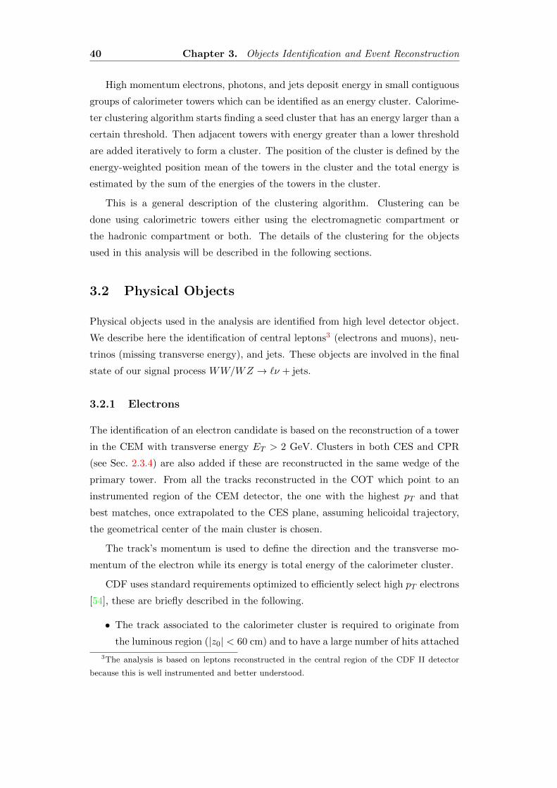
40 Chapter 3. Objects Identification and Event Reconstruction
High momentum electrons, photons, and jets deposit energy in small contiguous
groups of calorimeter towers which can be identified as an energy cluster. Calorime-
ter clustering algorithm starts finding a seed cluster that has an energy larger than a
certain threshold. Then adjacent towers with energy greater than a lower threshold
are added iteratively to form a cluster. The position of the cluster is defined by the
energy-weighted position mean of the towers in the cluster and the total energy is
estimated by the sum of the energies of the towers in the cluster.
This is a general description of the clustering algorithm. Clustering can be
done using calorimetric towers either using the electromagnetic compartment or
the hadronic compartment or both. The details of the clustering for the objects
used in this analysis will be described in the following sections.
3.2 Physical Objects
Physical objects used in the analysis are identified from high level detector object.
We describe here the identification of central leptons3 (electrons and muons), neu-
trinos (missing transverse energy), and jets. These objects are involved in the final
state of our signal process WW/WZ → `ν + jets.
3.2.1 Electrons
The identification of an electron candidate is based on the reconstruction of a tower
in the CEM with transverse energy ET > 2 GeV. Clusters in both CES and CPR
(see Sec. 2.3.4) are also added if these are reconstructed in the same wedge of the
primary tower. From all the tracks reconstructed in the COT which point to an
instrumented region of the CEM detector, the one with the highest pT and that
best matches, once extrapolated to the CES plane, assuming helicoidal trajectory,
the geometrical center of the main cluster is chosen.
The track’s momentum is used to define the direction and the transverse mo-
mentum of the electron while its energy is total energy of the calorimeter cluster.
CDF uses standard requirements optimized to efficiently select high pT electrons
[54], these are briefly described in the following.
• The track associated to the calorimeter cluster is required to originate from
the luminous region (|z0| < 60 cm) and to have a large number of hits attached
3The analysis is based on leptons reconstructed in the central region of the CDF II detector
because this is well instrumented and better understood.
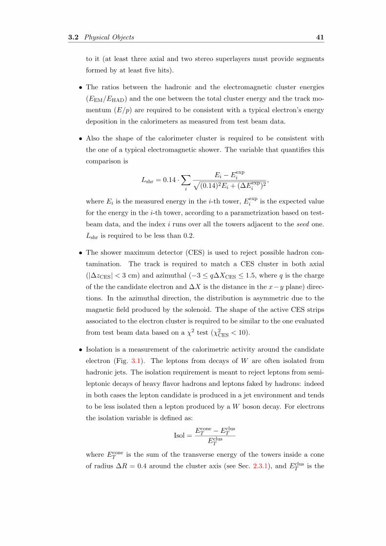
3.2 Physical Objects 41
to it (at least three axial and two stereo superlayers must provide segments
formed by at least five hits).
• The ratios between the hadronic and the electromagnetic cluster energies
(EEM/EHAD) and the one between the total cluster energy and the track mo-
mentum (E/p) are required to be consistent with a typical electron’s energy
deposition in the calorimeters as measured from test beam data.
• Also the shape of the calorimeter cluster is required to be consistent with
the one of a typical electromagnetic shower. The variable that quantifies this
comparison is
Lshr = 0.14 ·∑i
Ei − Eexpi√
(0.14)2Ei + (∆Eexpi )2
,
where Ei is the measured energy in the i-th tower, Eexpi is the expected value
for the energy in the i-th tower, according to a parametrization based on test-
beam data, and the index i runs over all the towers adjacent to the seed one.
Lshr is required to be less than 0.2.
• The shower maximum detector (CES) is used to reject possible hadron con-
tamination. The track is required to match a CES cluster in both axial
(|∆zCES| < 3 cm) and azimuthal (−3 ≤ q∆XCES ≤ 1.5, where q is the charge
of the the candidate electron and ∆X is the distance in the x−y plane) direc-
tions. In the azimuthal direction, the distribution is asymmetric due to the
magnetic field produced by the solenoid. The shape of the active CES strips
associated to the electron cluster is required to be similar to the one evaluated
from test beam data based on a χ2 test (χ2CES < 10).
• Isolation is a measurement of the calorimetric activity around the candidate
electron (Fig. 3.1). The leptons from decays of W are often isolated from
hadronic jets. The isolation requirement is meant to reject leptons from semi-
leptonic decays of heavy flavor hadrons and leptons faked by hadrons: indeed
in both cases the lepton candidate is produced in a jet environment and tends
to be less isolated then a lepton produced by a W boson decay. For electrons
the isolation variable is defined as:
Isol =EconeT − Eclus
T
EclusT
where EconeT is the sum of the transverse energy of the towers inside a cone
of radius ∆R = 0.4 around the cluster axis (see Sec. 2.3.1), and EclusT is the
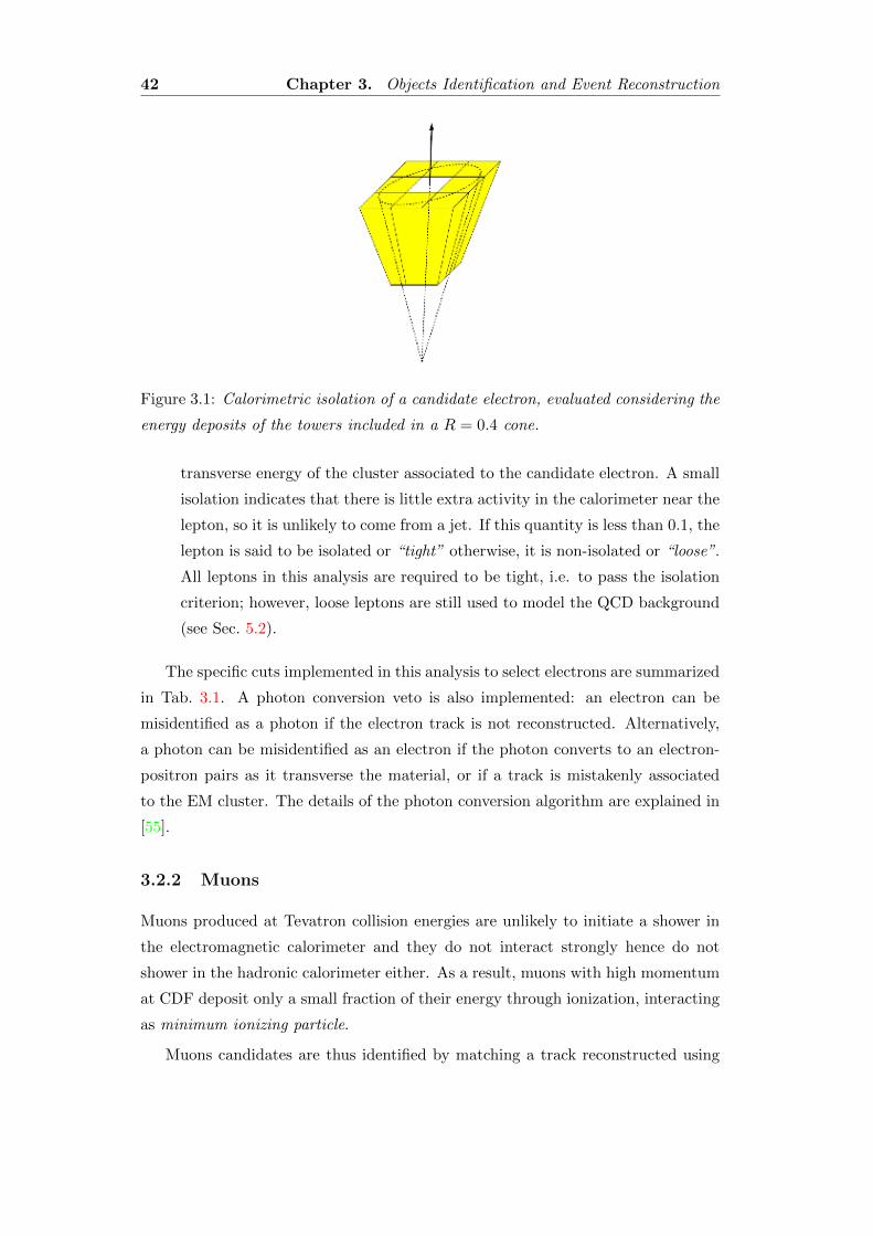
42 Chapter 3. Objects Identification and Event Reconstruction
Figure 3.1: Calorimetric isolation of a candidate electron, evaluated considering the
energy deposits of the towers included in a R = 0.4 cone.
transverse energy of the cluster associated to the candidate electron. A small
isolation indicates that there is little extra activity in the calorimeter near the
lepton, so it is unlikely to come from a jet. If this quantity is less than 0.1, the
lepton is said to be isolated or “tight” otherwise, it is non-isolated or “loose”.
All leptons in this analysis are required to be tight, i.e. to pass the isolation
criterion; however, loose leptons are still used to model the QCD background
(see Sec. 5.2).
The specific cuts implemented in this analysis to select electrons are summarized
in Tab. 3.1. A photon conversion veto is also implemented: an electron can be
misidentified as a photon if the electron track is not reconstructed. Alternatively,
a photon can be misidentified as an electron if the photon converts to an electron-
positron pairs as it transverse the material, or if a track is mistakenly associated
to the EM cluster. The details of the photon conversion algorithm are explained in
[55].
3.2.2 Muons
Muons produced at Tevatron collision energies are unlikely to initiate a shower in
the electromagnetic calorimeter and they do not interact strongly hence do not
shower in the hadronic calorimeter either. As a result, muons with high momentum
at CDF deposit only a small fraction of their energy through ionization, interacting
as minimum ionizing particle.
Muons candidates are thus identified by matching a track reconstructed using
3.2 Physical Objects 43
Variable Requirement
Fiduciality Detected in the active region of the CES/CEM
Track |Z0| ≤ 60 cm
ET > 20 GeV
pT > 10 GeV/c
COT Axial segments ≥ 3 with ≥ 5 hits each
COT Stereo segments ≥ 2 with ≥ 5 hits each
E/p ≤ 2 (unless pt ≥ 50 GeV/c)
EHAD/EEM ≤ 0.055 + 0.00043 · ELshr < 0.2
Iso/ET ≤ 0.1
Signed ∆XCES −3 ≤ q∆XCES ≤ 1.5
|∆zCES| < 3 cm
χ2CES ≤ 10
Table 3.1: Offline requirement for high pT central electrons [57].
the hits in the muon chambers (“stub”) with the extrapolation of reconstructed
track in the COT and requiring that little energy be deposited in the calorimeters
on the trajectory of the particle.
Real muons that are backgrounds for this analysis are: cosmic rays and muons
from decays in flight of kaons and charged pions or from heavy flavor semi-leptonic
decays. A veto, based on timing information from the muon chamber and the COT,
is used to reject cosmic rays events [56]. Muons can also be mimicked by hadrons
that shower unusually late or not at all in the calorimeter (“punch-through”).
In this analysis we define two types of muons according to the detector used to
identify them (see Sec. 2.3.6): CMX muons (with a stub in the CMX system that
covers the region 0.7 < |η| < 1) and CMUP muons (with a stub in both the CMU
and CMP systems with |η| < 0.7).
The observables and the requirements used to select the muons are briefly de-
scribed in the following [54] and summarized in Tab. 3.2.
• The quality of the COT track has the same requirements as for electrons.
Additionally, the track is required to have a low impact parameter (|d0| < 0.2
cm) in order to reject cosmic ray background. If hits from SVX are attached to
the track, the requirement on the impact parameter is more stringent (|d0| <
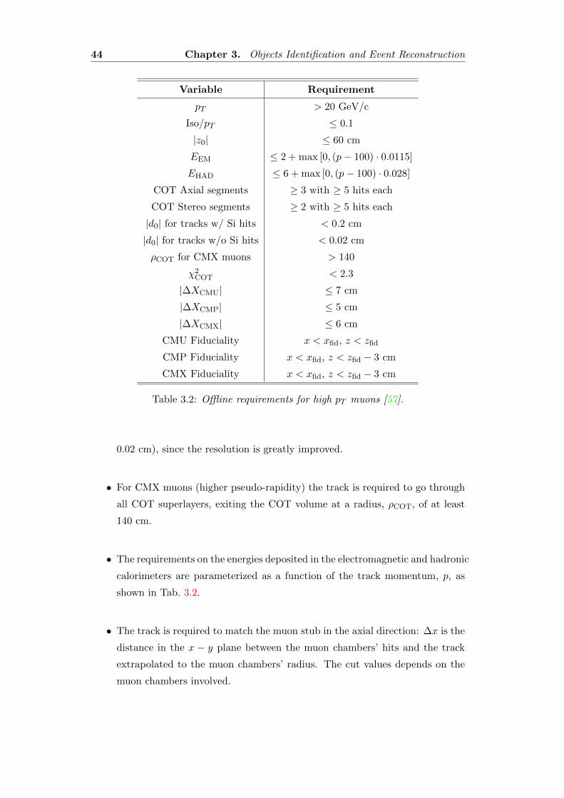
44 Chapter 3. Objects Identification and Event Reconstruction
Variable Requirement
pT > 20 GeV/c
Iso/pT ≤ 0.1
|z0| ≤ 60 cm
EEM ≤ 2 + max [0, (p− 100) · 0.0115]
EHAD ≤ 6 + max [0, (p− 100) · 0.028]
COT Axial segments ≥ 3 with ≥ 5 hits each
COT Stereo segments ≥ 2 with ≥ 5 hits each
|d0| for tracks w/ Si hits < 0.2 cm
|d0| for tracks w/o Si hits < 0.02 cm
ρCOT for CMX muons > 140
χ2COT < 2.3
|∆XCMU| ≤ 7 cm
|∆XCMP| ≤ 5 cm
|∆XCMX| ≤ 6 cm
CMU Fiduciality x < xfid, z < zfid
CMP Fiduciality x < xfid, z < zfid − 3 cm
CMX Fiduciality x < xfid, z < zfid − 3 cm
Table 3.2: Offline requirements for high pT muons [57].
0.02 cm), since the resolution is greatly improved.
• For CMX muons (higher pseudo-rapidity) the track is required to go through
all COT superlayers, exiting the COT volume at a radius, ρCOT, of at least
140 cm.
• The requirements on the energies deposited in the electromagnetic and hadronic
calorimeters are parameterized as a function of the track momentum, p, as
shown in Tab. 3.2.
• The track is required to match the muon stub in the axial direction: ∆x is the
distance in the x − y plane between the muon chambers’ hits and the track
extrapolated to the muon chambers’ radius. The cut values depends on the
muon chambers involved.
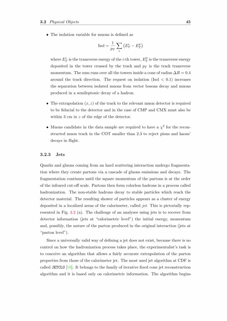
3.2 Physical Objects 45
• The isolation variable for muons is defined as
Isol =1
pT
∑i
(EiT − EµT
)where EiT is the transverse energy of the i-th tower, EµT is the transverse energy
deposited in the tower crossed by the track and pT is the track transverse
momentum. The sum runs over all the towers inside a cone of radius ∆R = 0.4
around the track direction. The request on isolation (Isol < 0.1) increases
the separation between isolated muons from vector bosons decay and muons
produced in a semileptonic decay of a hadron.
• The extrapolation (x, z) of the track to the relevant muon detector is required
to be fiducial to the detector and in the case of CMP and CMX must also be
within 3 cm in z of the edge of the detector.
• Muons candidate in the data sample are required to have a χ2 for the recon-
structed muon track in the COT smaller than 2.3 to reject pions and kaons’
decays in flight.
3.2.3 Jets
Quarks and gluons coming from an hard scattering interaction undergo fragmenta-
tion where they create partons via a cascade of gluons emissions and decays. The
fragmentation continues until the square momentum of the partons is at the order
of the infrared cut-off scale. Partons then form colorless hadrons in a process called
hadronization. The non-stable hadrons decay to stable particles which reach the
detector material. The resulting shower of particles appears as a cluster of energy
deposited in a localized areas of the calorimeter, called jet. This is pictorially rep-
resented in Fig. 3.2 (a). The challenge of an analyses using jets is to recover from
detector information (jets at “calorimetric level”) the initial energy, momentum
and, possibly, the nature of the parton produced in the original interaction (jets at
“parton level”).
Since a universally valid way of defining a jet does not exist, because there is no
control on how the hadronization process takes place, the experimentalist’s task is
to conceive an algorithm that allows a fairly accurate extrapolation of the parton
properties from those of the calorimeter jet. The most used jet algorithm at CDF is
called JETCLU [58]. It belongs to the family of iterative fixed cone jet reconstruction
algorithm and it is based only on calorimetric information. The algorithm begins
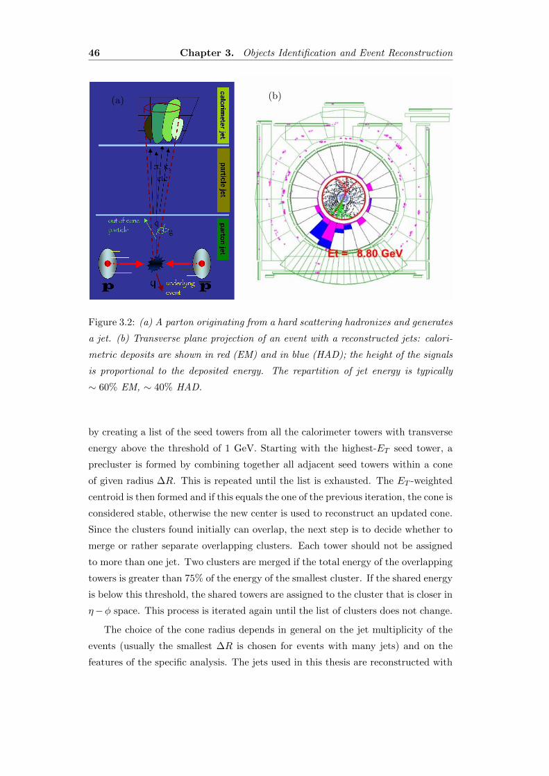
46 Chapter 3. Objects Identification and Event Reconstruction
(a) (b)
Figure 3.2: (a) A parton originating from a hard scattering hadronizes and generates
a jet. (b) Transverse plane projection of an event with a reconstructed jets: calori-
metric deposits are shown in red (EM) and in blue (HAD); the height of the signals
is proportional to the deposited energy. The repartition of jet energy is typically
∼ 60% EM, ∼ 40% HAD.
by creating a list of the seed towers from all the calorimeter towers with transverse
energy above the threshold of 1 GeV. Starting with the highest-ET seed tower, a
precluster is formed by combining together all adjacent seed towers within a cone
of given radius ∆R. This is repeated until the list is exhausted. The ET -weighted
centroid is then formed and if this equals the one of the previous iteration, the cone is
considered stable, otherwise the new center is used to reconstruct an updated cone.
Since the clusters found initially can overlap, the next step is to decide whether to
merge or rather separate overlapping clusters. Each tower should not be assigned
to more than one jet. Two clusters are merged if the total energy of the overlapping
towers is greater than 75% of the energy of the smallest cluster. If the shared energy
is below this threshold, the shared towers are assigned to the cluster that is closer in
η−φ space. This process is iterated again until the list of clusters does not change.
The choice of the cone radius depends in general on the jet multiplicity of the
events (usually the smallest ∆R is chosen for events with many jets) and on the
features of the specific analysis. The jets used in this thesis are reconstructed with

3.2 Physical Objects 47
∆R = 0.4.
Massless four-vector momenta are assigned to the towers in the clusters for
the electromagnetic and hadronic components, the jet four-vector is then defined
summing over all the towers in the cluster.
Jets Energy Corrections
The four-momentum assigned to a jet suffers for both detector inaccuracies and re-
construction algorithm imperfections. A set of corrections to the jet reconstructed
energy (“raw energy”) have been developed to partially overcome these limits, in
order to convert the measured transverse jet energy to the expected transverse en-
ergy of the partons. The corrections, assessed using data and simulation of the
CDF detector, include corrections for the response inhomogeneity in η, contribu-
tions from multiple interactions, the non- linearity of the calorimeter response, the
underlying event and the energy flow out of the jet cone. Each of those corrections
has a corresponding fractional uncertainty, σJES(pT ) which can be parameterized
as function of the corrected transverse momentum of the jet pT . They are applied
in a sequence of levels (of “L-levels’”) in order to correct for each bias independently
[59].
The correction can be parameterized as follows
ppartonT = (pjetT · Cη − CMI) · CAbs − CUE + COOC = pparticle
T − CUE + COOC ,
where the terms are described in the following.
Cη: pseudorapidity-dependent correction (L1) The L1 correction accounts
for non-uniformities in calorimeter response along η. This correction is ob-
tained by studying the pT balancing in dijet events. Dijet events are selected
in order to have one jet (“trigger jet”) in the 0.2 < |η| < 0.6 region (far away
from detector cracks). The other jet, called “probe jet”, is free to span over
the |η| < 3 region. The pT balancing fraction fb is formed and the correction
β is defined as
β =2 + 〈fb〉2− 〈fb〉
which is in average equal to pprobeT /ptrigger
T but reduces the sensitivity of the
measurement to the non-Gaussian tails which affect the latter ratio. The
uncertainty associated with this correction is estimated to be of the order of
1% for central jets and 7.5% for forward jets.
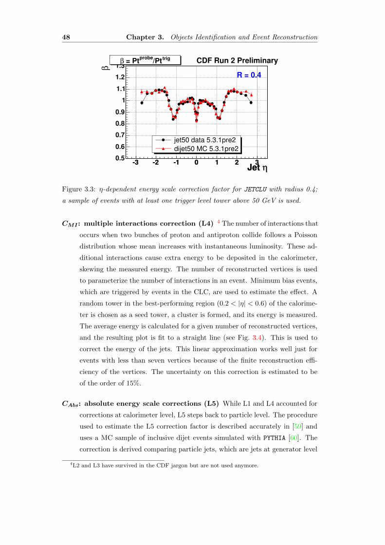
48 Chapter 3. Objects Identification and Event Reconstruction
ηJet -3 -2 -1 0 1 2 3
ηJet -3 -2 -1 0 1 2 3
β
0.5
0.6
0.7
0.8
0.9
1
1.1
1.2
1.3trig/Pt
probe = Ptβ
jet50 data 5.3.1pre2
dijet50 MC 5.3.1pre2
R = 0.4
CDF Run 2 Preliminarytrig/Ptprobe
= Ptβ
Figure 3.3: η-dependent energy scale correction factor for JETCLU with radius 0.4;
a sample of events with at least one trigger level tower above 50 GeV is used.
CMI : multiple interactions correction (L4) 4 The number of interactions that
occurs when two bunches of proton and antiproton collide follows a Poisson
distribution whose mean increases with instantaneous luminosity. These ad-
ditional interactions cause extra energy to be deposited in the calorimeter,
skewing the measured energy. The number of reconstructed vertices is used
to parameterize the number of interactions in an event. Minimum bias events,
which are triggered by events in the CLC, are used to estimate the effect. A
random tower in the best-performing region (0.2 < |η| < 0.6) of the calorime-
ter is chosen as a seed tower, a cluster is formed, and its energy is measured.
The average energy is calculated for a given number of reconstructed vertices,
and the resulting plot is fit to a straight line (see Fig. 3.4). This is used to
correct the energy of the jets. This linear approximation works well just for
events with less than seven vertices because of the finite reconstruction effi-
ciency of the vertices. The uncertainty on this correction is estimated to be
of the order of 15%.
CAbs: absolute energy scale corrections (L5) While L1 and L4 accounted for
corrections at calorimeter level, L5 steps back to particle level. The procedure
used to estimate the L5 correction factor is described accurately in [59] and
uses a MC sample of inclusive dijet events simulated with PYTHIA [60]. The
correction is derived comparing particle jets, which are jets at generator level
4L2 and L3 have survived in the CDF jargon but are not used anymore.
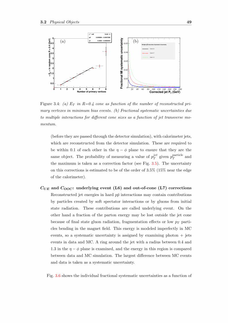
3.2 Physical Objects 49
Number of primary vertices0 1 2 3 4 5 6 7 8
> in
ran
do
m c
on
e R
= 0
.4 (
GeV
)T
< E
0.5
1
1.5
2
2.5
3
3.5
4
4.5
5
/ ndf 2χ 15.62 / 4
p0 0.0007298± 0.005894
p1 0.0006464± 0.3563
/ ndf 2χ 15.62 / 4
p0 0.0007298± 0.005894
p1 0.0006464± 0.3563 (a)
(GeV)TCorrected jet P20 40 60 80 100 120 140 160 180 200
Fra
cti
on
al
MI
sy
ste
ma
tic
un
ce
rta
inty
0
0.01
0.02
0.03
0.04
0.05 Interactions Systematic UncertaintypMultiple p
Cone 0.4
Cone 0.7
Cone 1.0
Interactions Systematic UncertaintypMultiple p
Cone 0.4
Cone 0.7
Cone 1.0
(b)
Figure 3.4: (a) ET in R=0.4 cone as function of the number of reconstructed pri-
mary vertexes in minimum bias events. (b) Fractional systematic uncertainties due
to multiple interactions for different cone sizes as a function of jet transverse mo-
mentum.
(before they are passed through the detector simulation), with calorimeter jets,
which are reconstructed from the detector simulation. These are required to
be within 0.1 of each other in the η − φ plane to ensure that they are the
same object. The probability of measuring a value of pjetT given pparticleT and
the maximum is taken as a correction factor (see Fig. 3.5). The uncertainty
on this corrections is estimated to be of the order of 3.5% (15% near the edge
of the calorimeter).
CUE and COOC : underlying event (L6) and out-of-cone (L7) corrections
Reconstructed jet energies in hard pp interactions may contain contributions
by particles created by soft spectator interactions or by gluons from initial
state radiation. These contributions are called underlying event. On the
other hand a fraction of the parton energy may be lost outside the jet cone
because of final state gluon radiation, fragmentation effects or low pT parti-
cles bending in the magnet field. This energy is modeled imperfectly in MC
events, so a systematic uncertainty is assigned by examining photon + jets
events in data and MC. A ring around the jet with a radius between 0.4 and
1.3 in the η − φ plane is examined, and the energy in this region is compared
between data and MC simulation. The largest difference between MC events
and data is taken as a systematic uncertainty.
Fig. 3.6 shows the individual fractional systematic uncertainties as a function of
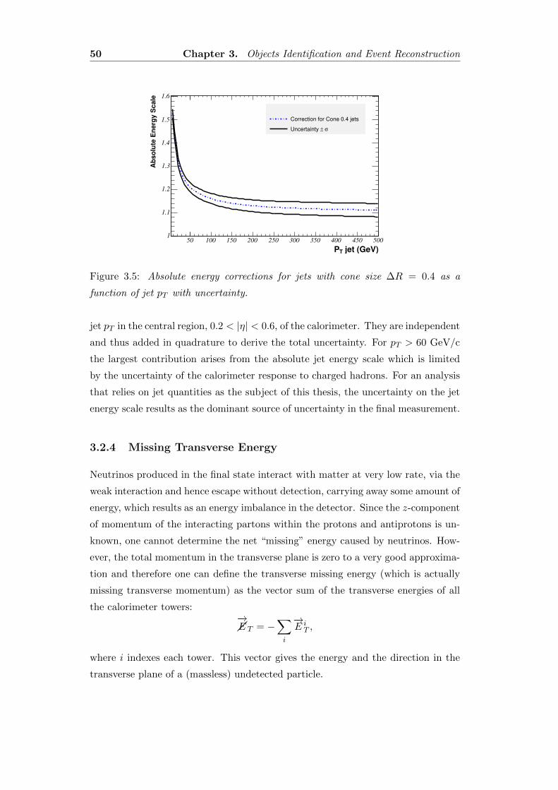
50 Chapter 3. Objects Identification and Event Reconstruction
jet (GeV)TP50 100 150 200 250 300 350 400 450 500
Ab
so
lute
En
erg
y S
cale
1
1.1
1.2
1.3
1.4
1.5
1.6
Correction for Cone 0.4 jets
σ ±Uncertainty
Correction for Cone 0.4 jets
σ ±Uncertainty
Figure 3.5: Absolute energy corrections for jets with cone size ∆R = 0.4 as a
function of jet pT with uncertainty.
jet pT in the central region, 0.2 < |η| < 0.6, of the calorimeter. They are independent
and thus added in quadrature to derive the total uncertainty. For pT > 60 GeV/c
the largest contribution arises from the absolute jet energy scale which is limited
by the uncertainty of the calorimeter response to charged hadrons. For an analysis
that relies on jet quantities as the subject of this thesis, the uncertainty on the jet
energy scale results as the dominant source of uncertainty in the final measurement.
3.2.4 Missing Transverse Energy
Neutrinos produced in the final state interact with matter at very low rate, via the
weak interaction and hence escape without detection, carrying away some amount of
energy, which results as an energy imbalance in the detector. Since the z-component
of momentum of the interacting partons within the protons and antiprotons is un-
known, one cannot determine the net “missing” energy caused by neutrinos. How-
ever, the total momentum in the transverse plane is zero to a very good approxima-
tion and therefore one can define the transverse missing energy (which is actually
missing transverse momentum) as the vector sum of the transverse energies of all
the calorimeter towers:−→��E T = −
∑i
−→E iT ,
where i indexes each tower. This vector gives the energy and the direction in the
transverse plane of a (massless) undetected particle.
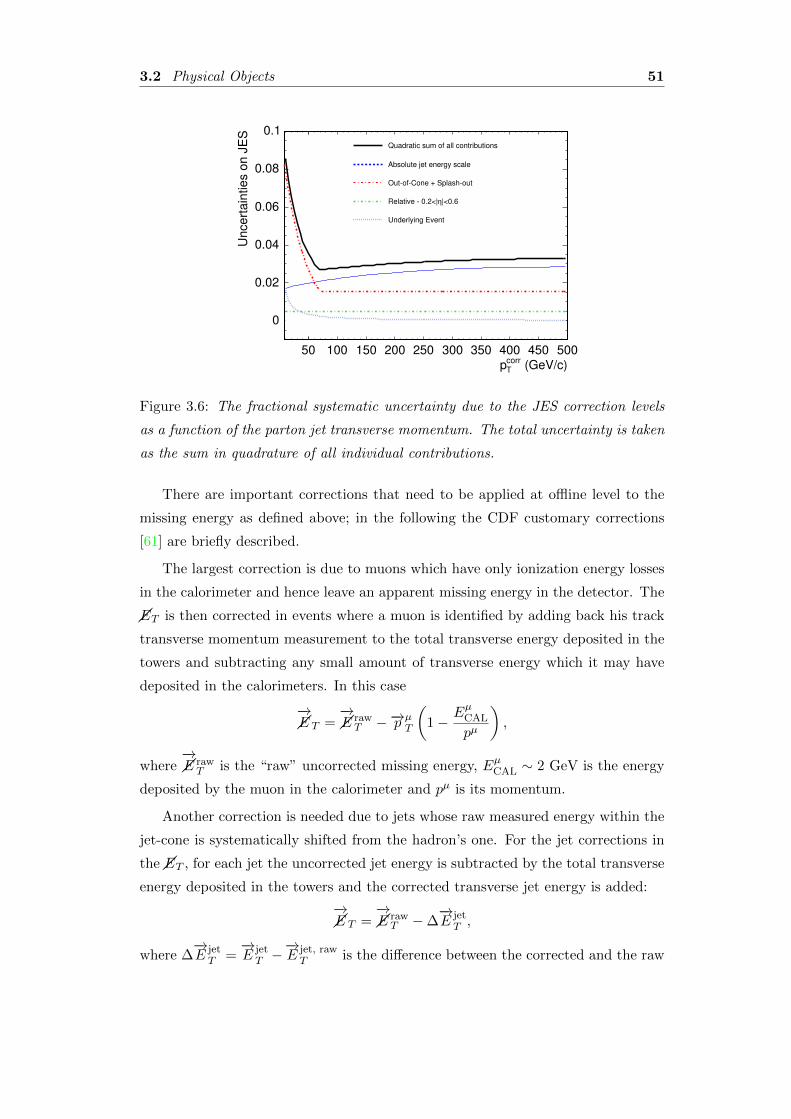
3.2 Physical Objects 51
(GeV/c)corrTp
50 100 150 200 250 300 350 400 450 500
Uncert
ain
ties o
n J
ES
0
0.02
0.04
0.06
0.08
0.1Quadratic sum of all contributions
Absolute jet energy scale
Out-of-Cone + Splash-out
|<0.6ηRelative - 0.2<|
Underlying Event
Figure 3.6: The fractional systematic uncertainty due to the JES correction levels
as a function of the parton jet transverse momentum. The total uncertainty is taken
as the sum in quadrature of all individual contributions.
There are important corrections that need to be applied at offline level to the
missing energy as defined above; in the following the CDF customary corrections
[61] are briefly described.
The largest correction is due to muons which have only ionization energy losses
in the calorimeter and hence leave an apparent missing energy in the detector. The
��ET is then corrected in events where a muon is identified by adding back his track
transverse momentum measurement to the total transverse energy deposited in the
towers and subtracting any small amount of transverse energy which it may have
deposited in the calorimeters. In this case
−→��E T =
−→��E
rawT −−→p µT
(1− EµCAL
pµ
),
where−→��E
rawT is the “raw” uncorrected missing energy, EµCAL ∼ 2 GeV is the energy
deposited by the muon in the calorimeter and pµ is its momentum.
Another correction is needed due to jets whose raw measured energy within the
jet-cone is systematically shifted from the hadron’s one. For the jet corrections in
the ��ET , for each jet the uncorrected jet energy is subtracted by the total transverse
energy deposited in the towers and the corrected transverse jet energy is added:
−→��E T =
−→��E
rawT −∆
−→E jetT ,
where ∆−→E jetT =
−→E jetT −
−→E jet, rawT is the difference between the corrected and the raw

52 Chapter 3. Objects Identification and Event Reconstruction
energies of the jet.
The source of real ��ET in this analysis is from neutrinos created in electroweak
interactions. There are also several sources of false ��ET which are often difficult to
control. These sources include the mis-measurement of jet and lepton energies as
well as when a lepton or photon or hadron enters a crack in the detector where
it would not be possible to reconstruct its energy with any reasonable accuracy.
Dealing with this requires some care in reconstructing the neutrino.
Chapter 4
Event Selection
In this chapter we describe the details of the offline selection based on the physical
object reconstruction performed in the previous chapter. The criteria are designed
to efficiently select our signal events and reduce the backgrounds that share the
same signature (lepton, ��ET and jets).
4.1 Signal and Background Definition
The events of interest for this analysis have the experimental signature of semi-
leptonic WW and WZ decays which consists of at least two energetic jets, a high
pT isolated lepton (electron or muon) and large missing transverse energy. A typical
candidate event with this signature is shown in Fig. 4.1.
Several other processes have the same signature (either processes that have a
lepton from a W decay or whose signatures fakes the lepton from the W ) so they
are considered as backgrounds of our signal process:
• W+jets: the main background is the production of W boson in association
with multiple high ET jets,
pp→W± → `±ν` + jets.
W bosons are produced in pp interaction mostly by processes where a quark
from a proton and antiquark from an antiproton annihilate in a W boson.
QCD radiation from the colliding partons easily produce multiple high pT
partons in association with the W boson. There are several Feynman dia-
grams (Fig. 4.2 shows one of them) leading to this final state but the detailed
53
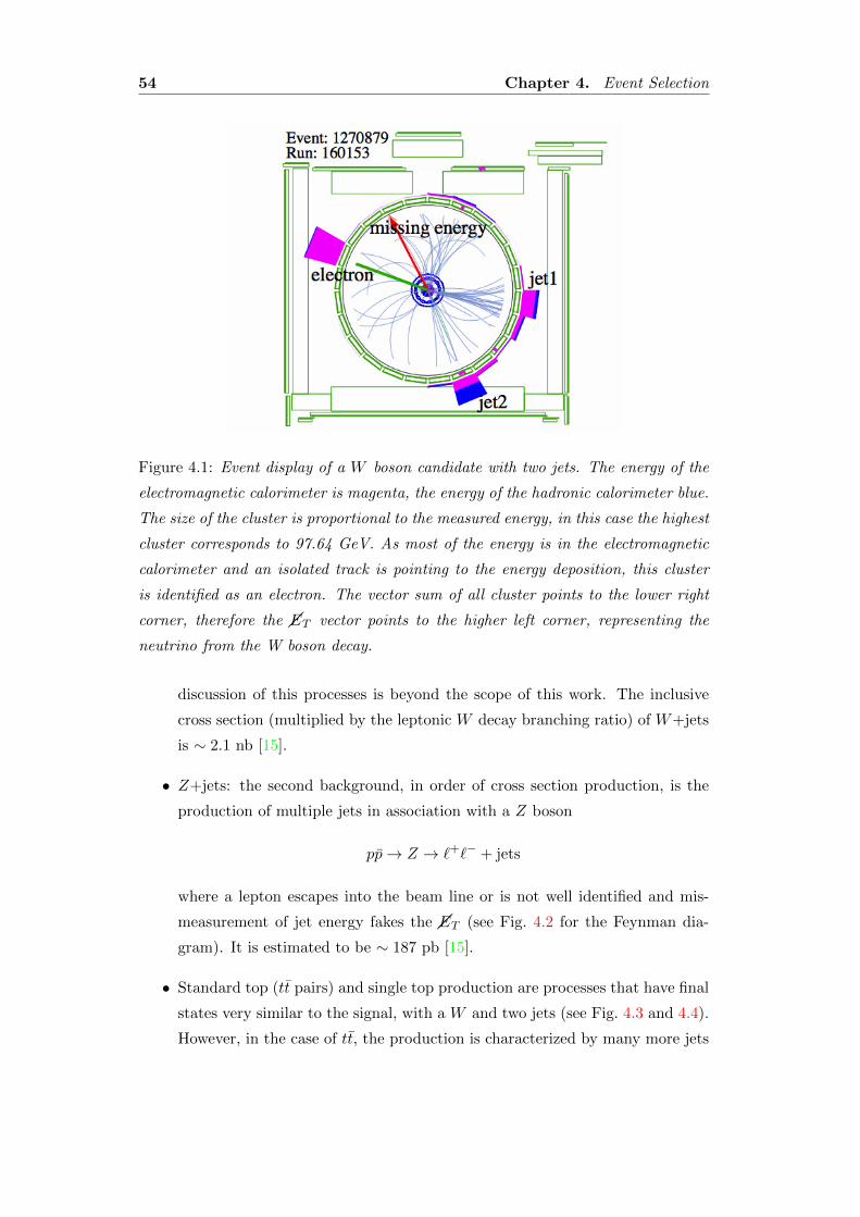
54 Chapter 4. Event Selection
Figure 4.1: Event display of a W boson candidate with two jets. The energy of the
electromagnetic calorimeter is magenta, the energy of the hadronic calorimeter blue.
The size of the cluster is proportional to the measured energy, in this case the highest
cluster corresponds to 97.64 GeV. As most of the energy is in the electromagnetic
calorimeter and an isolated track is pointing to the energy deposition, this cluster
is identified as an electron. The vector sum of all cluster points to the lower right
corner, therefore the ��ET vector points to the higher left corner, representing the
neutrino from the W boson decay.
discussion of this processes is beyond the scope of this work. The inclusive
cross section (multiplied by the leptonic W decay branching ratio) of W+jets
is ∼ 2.1 nb [15].
• Z+jets: the second background, in order of cross section production, is the
production of multiple jets in association with a Z boson
pp→ Z → `+`− + jets
where a lepton escapes into the beam line or is not well identified and mis-
measurement of jet energy fakes the ��ET (see Fig. 4.2 for the Feynman dia-
gram). It is estimated to be ∼ 187 pb [15].
• Standard top (tt pairs) and single top production are processes that have final
states very similar to the signal, with a W and two jets (see Fig. 4.3 and 4.4).
However, in the case of tt, the production is characterized by many more jets
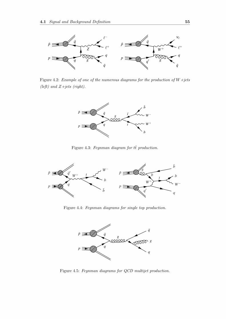
4.1 Signal and Background Definition 55
q
q
Z
gp
p
q
q
ℓ+
ℓ−
q′
q
W+
gp
p
q
q
ℓ+
νℓ
Figure 4.2: Example of one of the numerous diagrams for the production of W+jets
(left) and Z+jets (right).
q
qg
t
t
p
p
b
W+
W−
b
Figure 4.3: Feynman diagram for tt production.
q
q′W+ t
p
p
b
b
W−
q′
g
bt
W+
p
p
q
W−
b
b
Figure 4.4: Feynman diagrams for single top production.
q
qg
p
p
q
g
q
Figure 4.5: Feynman diagrams for QCD multijet production.
56 Chapter 4. Event Selection
in the final state that will give an handle to discriminate signal from this
background. The corresponding cross section are [62] [63]
σ(pp→ tt) = 7.5 pb
σ(pp→ tb) = 2.9 pb
• QCD multijet: the most difficult events to model come from QCD multijet
events (see Fig. 4.5). The extremely large cross section of QCD multijet events
means that even kinematically unlikely configurations can form a significant
background. In particular, highly unlikely events needed to fake the neces-
sary signature (a three-jet event in which one jet manages to pass all lepton
cuts and, simultaneously, the energies are so poorly measured that a large
missing transverse energy is reported) still occurs with enough probability to
contaminate the sample significantly. Because of the extremely small rate of
these events to occur, and because they come from different QCD processes,
that are difficult to calculate or model, it is highly unreliable to simulate these
events with MC events and we need to derive the model directly from the data
(see Sec. 5.2).
The large cross section of these processes leads to a large contamination of
different backgrounds in the data sample. Dedicated online and offline selections
are needed to improve the signal over background ratio.
4.2 Data Sample
This analysis uses 4.3 fb−1 of data collected by CDF II detector between February
2002 and March 2009. The datasets used have been selected by any of the triggers
for high pT central leptons, ELECTRON CENTRAL 18, MUON CMUP 18 and MUON CMX 18
(see following section) and spans run1 numbers from 138425 to 274055.
Only “good runs”, where all components of the detector relevant for this analysis
are reliably working, are included. Each dataset is organized in more secondary
datasets corresponding to different data periods during which the detector was
operated under a stable configuration (i.e. trigger settings, average instantaneous
luminosity, system calibrations, etc. can change over time).
1A run is a period of continuous operation of the CDF II Data Acquisition. Many different
cases can require the DAQ to be stopped and restarted including the need to enable or disable a
sub-detector, a change in the trigger Table, a problem in the trigger/DAQ chain etc.
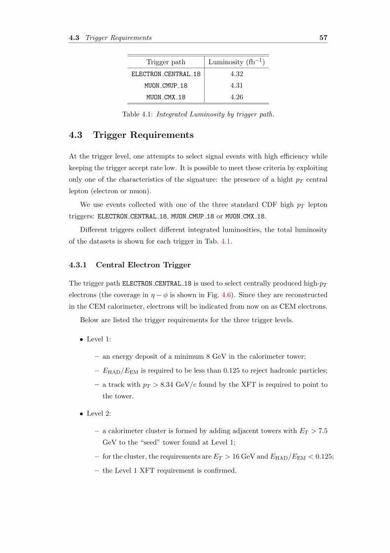
4.3 Trigger Requirements 57
Trigger path Luminosity (fb−1)
ELECTRON CENTRAL 18 4.32
MUON CMUP 18 4.31
MUON CMX 18 4.26
Table 4.1: Integrated Luminosity by trigger path.
4.3 Trigger Requirements
At the trigger level, one attempts to select signal events with high efficiency while
keeping the trigger accept rate low. It is possible to meet these criteria by exploiting
only one of the characteristics of the signature: the presence of a hight pT central
lepton (electron or muon).
We use events collected with one of the three standard CDF high pT lepton
triggers: ELECTRON CENTRAL 18, MUON CMUP 18 or MUON CMX 18.
Different triggers collect different integrated luminosities, the total luminosity
of the datasets is shown for each trigger in Tab. 4.1.
4.3.1 Central Electron Trigger
The trigger path ELECTRON CENTRAL 18 is used to select centrally produced high-pT
electrons (the coverage in η − φ is shown in Fig. 4.6). Since they are reconstructed
in the CEM calorimeter, electrons will be indicated from now on as CEM electrons.
Below are listed the trigger requirements for the three trigger levels.
• Level 1:
– an energy deposit of a minimum 8 GeV in the calorimeter tower;
– EHAD/EEM is required to be less than 0.125 to reject hadronic particles;
– a track with pT > 8.34 GeV/c found by the XFT is required to point to
the tower.
• Level 2:
– a calorimeter cluster is formed by adding adjacent towers with ET > 7.5
GeV to the “seed” tower found at Level 1;
– for the cluster, the requirements are ET > 16 GeV and EHAD/EEM < 0.125;
– the Level 1 XFT requirement is confirmed.
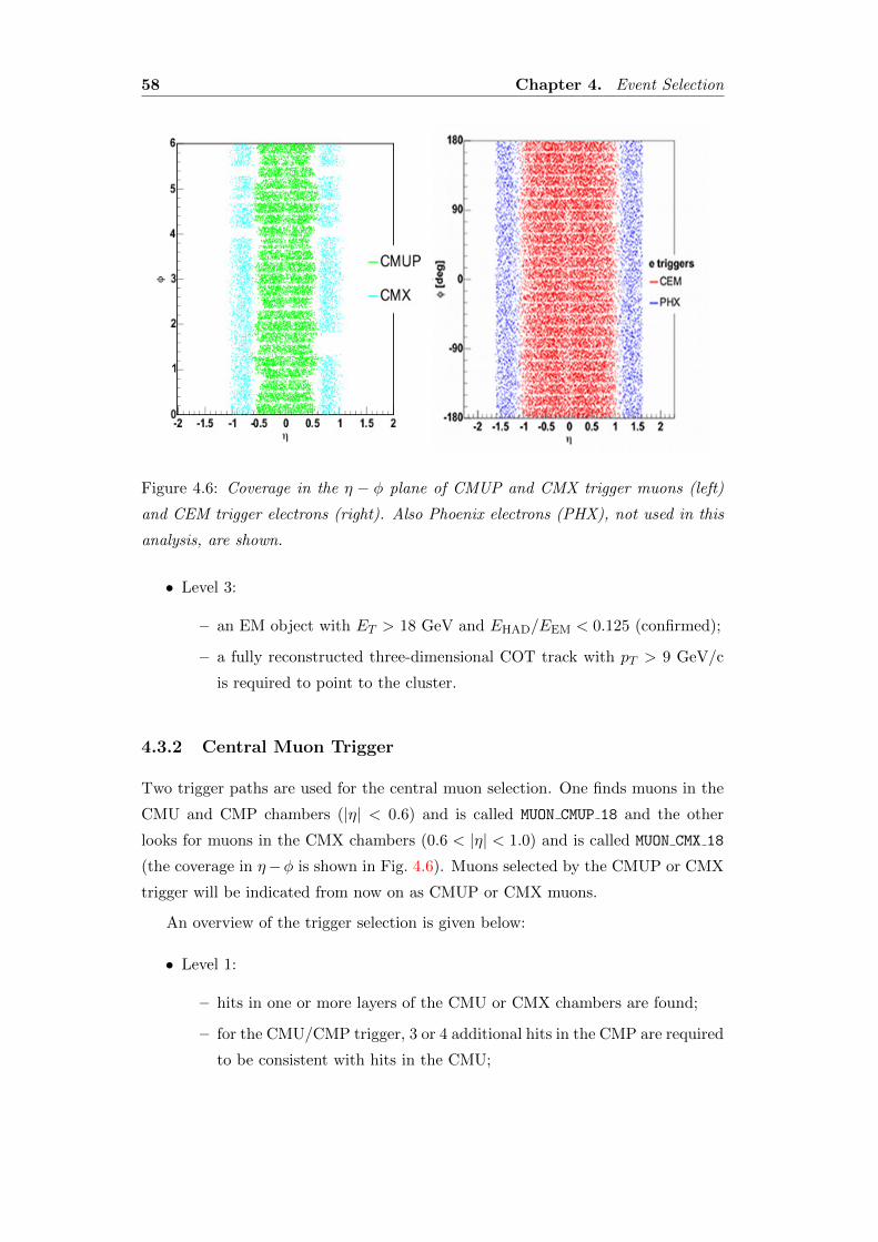
58 Chapter 4. Event Selection
Figure 4.6: Coverage in the η − φ plane of CMUP and CMX trigger muons (left)
and CEM trigger electrons (right). Also Phoenix electrons (PHX), not used in this
analysis, are shown.
• Level 3:
– an EM object with ET > 18 GeV and EHAD/EEM < 0.125 (confirmed);
– a fully reconstructed three-dimensional COT track with pT > 9 GeV/c
is required to point to the cluster.
4.3.2 Central Muon Trigger
Two trigger paths are used for the central muon selection. One finds muons in the
CMU and CMP chambers (|η| < 0.6) and is called MUON CMUP 18 and the other
looks for muons in the CMX chambers (0.6 < |η| < 1.0) and is called MUON CMX 18
(the coverage in η−φ is shown in Fig. 4.6). Muons selected by the CMUP or CMX
trigger will be indicated from now on as CMUP or CMX muons.
An overview of the trigger selection is given below:
• Level 1:
– hits in one or more layers of the CMU or CMX chambers are found;
– for the CMU/CMP trigger, 3 or 4 additional hits in the CMP are required
to be consistent with hits in the CMU;
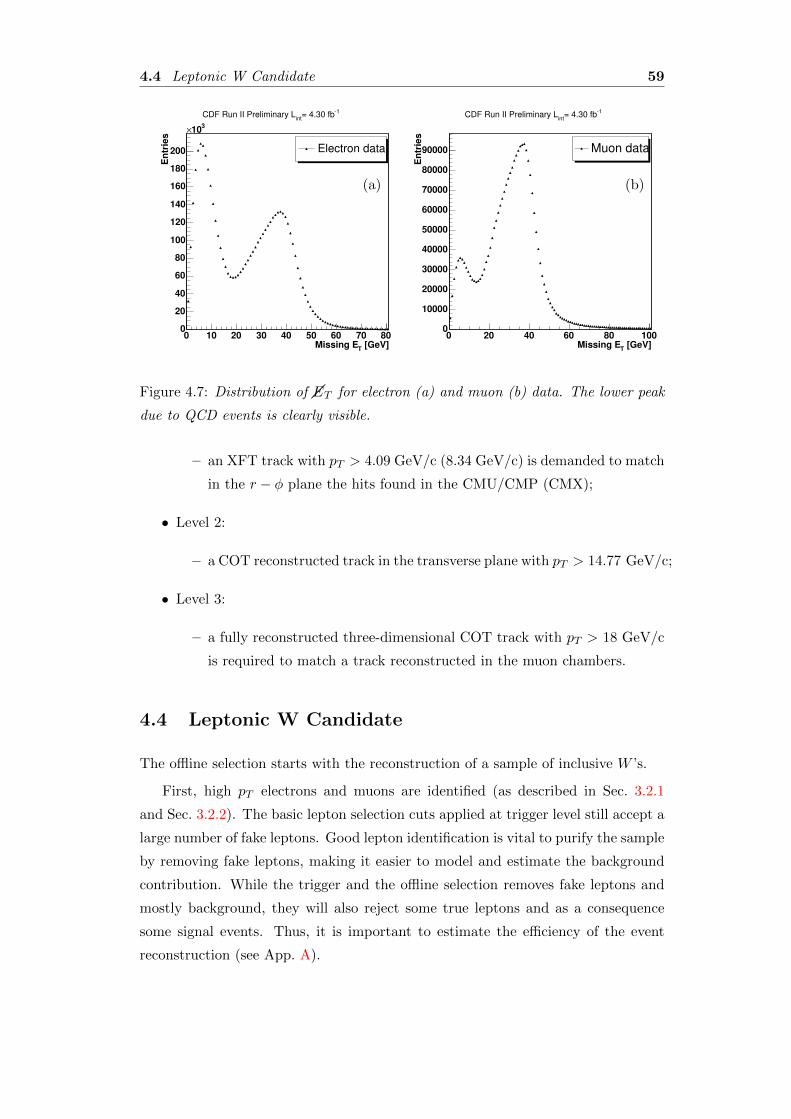
4.4 Leptonic W Candidate 59
[GeV]T
Missing E0 10 20 30 40 50 60 70 80
En
trie
s
0
20
40
60
80
100
120
140
160
180
200
310×
-1= 4.30 fbint
CDF Run II Preliminary L
Electron data
(a)
[GeV]T
Missing E0 20 40 60 80 100
En
trie
s
0
10000
20000
30000
40000
50000
60000
70000
80000
90000
-1= 4.30 fbint
CDF Run II Preliminary L
Muon data
(b)
Figure 4.7: Distribution of ��ET for electron (a) and muon (b) data. The lower peak
due to QCD events is clearly visible.
– an XFT track with pT > 4.09 GeV/c (8.34 GeV/c) is demanded to match
in the r − φ plane the hits found in the CMU/CMP (CMX);
• Level 2:
– a COT reconstructed track in the transverse plane with pT > 14.77 GeV/c;
• Level 3:
– a fully reconstructed three-dimensional COT track with pT > 18 GeV/c
is required to match a track reconstructed in the muon chambers.
4.4 Leptonic W Candidate
The offline selection starts with the reconstruction of a sample of inclusive W ’s.
First, high pT electrons and muons are identified (as described in Sec. 3.2.1
and Sec. 3.2.2). The basic lepton selection cuts applied at trigger level still accept a
large number of fake leptons. Good lepton identification is vital to purify the sample
by removing fake leptons, making it easier to model and estimate the background
contribution. While the trigger and the offline selection removes fake leptons and
mostly background, they will also reject some true leptons and as a consequence
some signal events. Thus, it is important to estimate the efficiency of the event
reconstruction (see App. A).
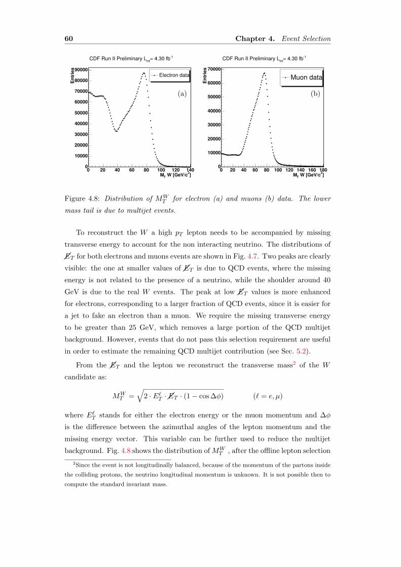
60 Chapter 4. Event Selection
]2
W [GeV/cT
M0 20 40 60 80 100 120 140
En
trie
s
0
10000
20000
30000
40000
50000
60000
70000
80000
90000
-1= 4.30 fbint
CDF Run II Preliminary L
Electron data
(a)
]2
W [GeV/cT
M0 20 40 60 80 100 120 140 160 180
En
trie
s
0
10000
20000
30000
40000
50000
60000
70000
-1= 4.30 fbint
CDF Run II Preliminary L
Muon data
(b)
Figure 4.8: Distribution of MWT for electron (a) and muons (b) data. The lower
mass tail is due to multijet events.
To reconstruct the W a high pT lepton needs to be accompanied by missing
transverse energy to account for the non interacting neutrino. The distributions of
��ET for both electrons and muons events are shown in Fig. 4.7. Two peaks are clearly
visible: the one at smaller values of ��ET is due to QCD events, where the missing
energy is not related to the presence of a neutrino, while the shoulder around 40
GeV is due to the real W events. The peak at low ��ET values is more enhanced
for electrons, corresponding to a larger fraction of QCD events, since it is easier for
a jet to fake an electron than a muon. We require the missing transverse energy
to be greater than 25 GeV, which removes a large portion of the QCD multijet
background. However, events that do not pass this selection requirement are useful
in order to estimate the remaining QCD multijet contribution (see Sec. 5.2).
From the ��ET and the lepton we reconstruct the transverse mass2 of the W
candidate as:
MWT =
√2 · E`T ·��ET · (1− cos ∆φ) (` = e, µ)
where E`T stands for either the electron energy or the muon momentum and ∆φ
is the difference between the azimuthal angles of the lepton momentum and the
missing energy vector. This variable can be further used to reduce the multijet
background. Fig. 4.8 shows the distribution of MWT , after the offline lepton selection
2Since the event is not longitudinally balanced, because of the momentum of the partons inside
the colliding protons, the neutrino longitudinal momentum is unknown. It is not possible then to
compute the standard invariant mass.
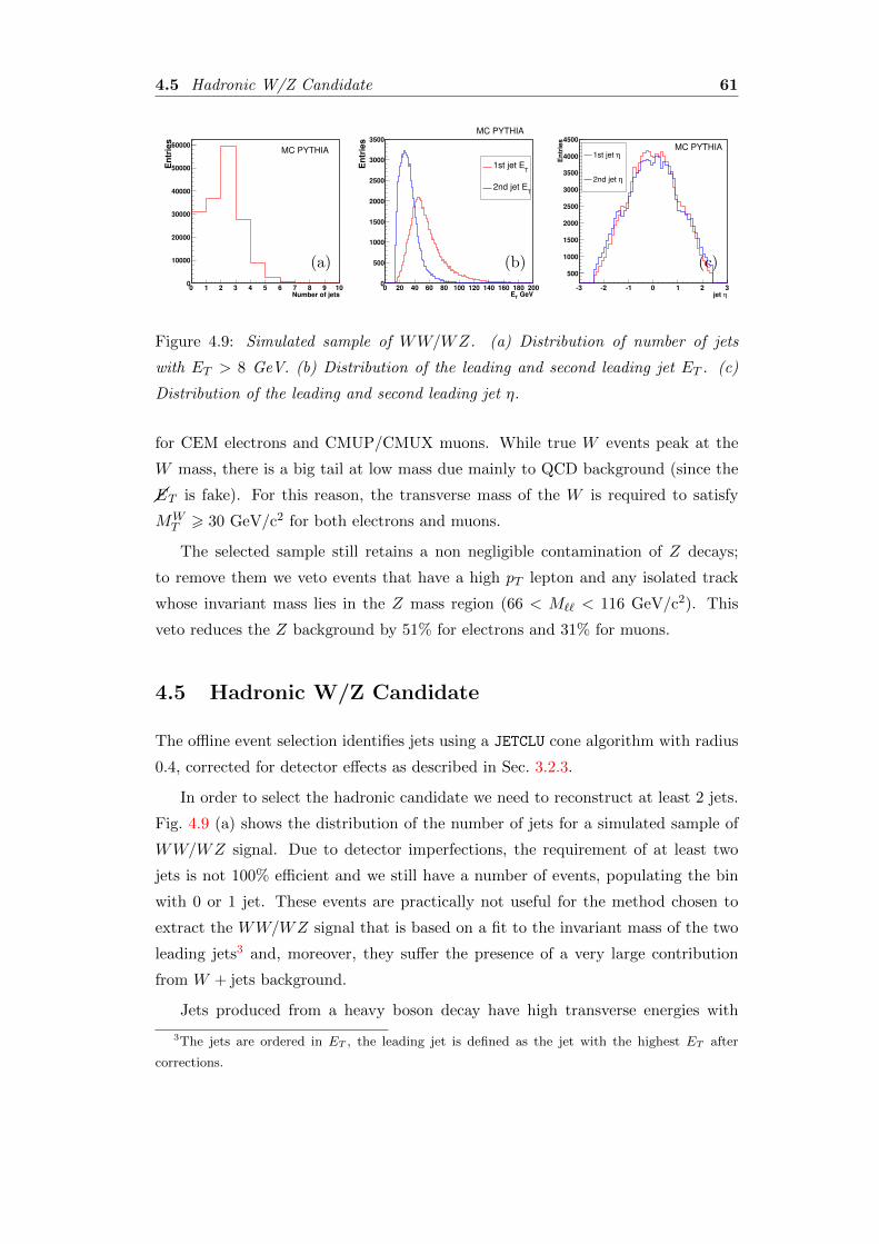
4.5 Hadronic W/Z Candidate 61
Number of jets0 1 2 3 4 5 6 7 8 9 10
En
trie
s
0
10000
20000
30000
40000
50000
60000MC PYTHIA
(a)
GeVT
E0 20 40 60 80 100 120 140 160 180 200
En
trie
s
0
500
1000
1500
2000
2500
3000
3500
MC PYTHIA
T1st jet E
T2nd jet E
(b)
ηjet 3 2 1 0 1 2 3
En
trie
s
500
1000
1500
2000
2500
3000
3500
4000
4500
MC PYTHIAη1st jet
η2nd jet
(c)
Figure 4.9: Simulated sample of WW/WZ. (a) Distribution of number of jets
with ET > 8 GeV. (b) Distribution of the leading and second leading jet ET . (c)
Distribution of the leading and second leading jet η.
for CEM electrons and CMUP/CMUX muons. While true W events peak at the
W mass, there is a big tail at low mass due mainly to QCD background (since the
��ET is fake). For this reason, the transverse mass of the W is required to satisfy
MWT > 30 GeV/c2 for both electrons and muons.
The selected sample still retains a non negligible contamination of Z decays;
to remove them we veto events that have a high pT lepton and any isolated track
whose invariant mass lies in the Z mass region (66 < M`` < 116 GeV/c2). This
veto reduces the Z background by 51% for electrons and 31% for muons.
4.5 Hadronic W/Z Candidate
The offline event selection identifies jets using a JETCLU cone algorithm with radius
0.4, corrected for detector effects as described in Sec. 3.2.3.
In order to select the hadronic candidate we need to reconstruct at least 2 jets.
Fig. 4.9 (a) shows the distribution of the number of jets for a simulated sample of
WW/WZ signal. Due to detector imperfections, the requirement of at least two
jets is not 100% efficient and we still have a number of events, populating the bin
with 0 or 1 jet. These events are practically not useful for the method chosen to
extract the WW/WZ signal that is based on a fit to the invariant mass of the two
leading jets3 and, moreover, they suffer the presence of a very large contribution
from W + jets background.
Jets produced from a heavy boson decay have high transverse energies with
3The jets are ordered in ET , the leading jet is defined as the jet with the highest ET after
corrections.
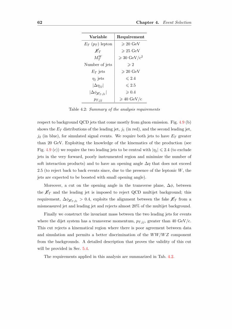
62 Chapter 4. Event Selection
Variable Requirement
ET (pT ) lepton > 20 GeV
��ET > 25 GeV
MWT > 30 GeV/c2
Number of jets > 2
ET jets > 20 GeV
ηj jets 6 2.4
|∆ηjj | 6 2.5
|∆φ�ET ,j1 | > 0.4
pT,jj > 40 GeV/c
Table 4.2: Summary of the analysis requirements
respect to background QCD jets that come mostly from gluon emission. Fig. 4.9 (b)
shows the ET distributions of the leading jet, j1 (in red), and the second leading jet,
j2 (in blue), for simulated signal events. We require both jets to have ET greater
than 20 GeV. Exploiting the knowledge of the kinematics of the production (see
Fig. 4.9 (c)) we require the two leading jets to be central with |ηj | 6 2.4 (to exclude
jets in the very forward, poorly instrumented region and minimize the number of
soft interaction products) and to have an opening angle ∆η that does not exceed
2.5 (to reject back to back events since, due to the presence of the leptonic W , the
jets are expected to be boosted with small opening angle).
Moreover, a cut on the opening angle in the transverse plane, ∆φ, between
the ��ET and the leading jet is imposed to reject QCD multijet background; this
requirement, ∆φ�ET ,j1 > 0.4, exploits the alignment between the fake ��ET from a
mismeasured jet and leading jet and rejects almost 20% of the multijet background.
Finally we construct the invariant mass between the two leading jets for events
where the dijet system has a transverse momentum, pT,jj , greater than 40 GeV/c.
This cut rejects a kinematical region where there is poor agreement between data
and simulation and permits a better discrimination of the WW/WZ component
from the backgrounds. A detailed description that proves the validity of this cut
will be provided in Sec. 5.4.
The requirements applied in this analysis are summarized in Tab. 4.2.
Chapter 5
Sample Composition and
Modeling
This analysis uses a fit to the invariant mass distribution of the two leading jets
associated to the hadronic decay of W/Z boson to disentangle the diboson signal
from the backgrounds in the data sample selected in the previous chapter. The
sensitivity to the signal and its significance rely on an accurate modeling of each
contributing component in the fit.
This chapter will discuss the methods used to model the data and to estimate
the event yield of each contributing process.
5.1 MC-Based Processes
For any process with a well understood cross section, the yield estimate is derived
from the MC simulation (details about the simulation can be found in App. B).
These processes include the single top, tt, diboson and Z+jets.
The determination of the predicted events for each process starts from the calcu-
lation of its acceptance. The acceptance is derived from the simulated MC samples
as the fraction of events passing all the event selection cuts. This number needs to
be corrected in order to take into account the differences between the simulation
and the real experimental setup. A weight is given to each MC sample:
w =
∫Ldt · εtrig · SFreco ·
σpredNevt
where
63
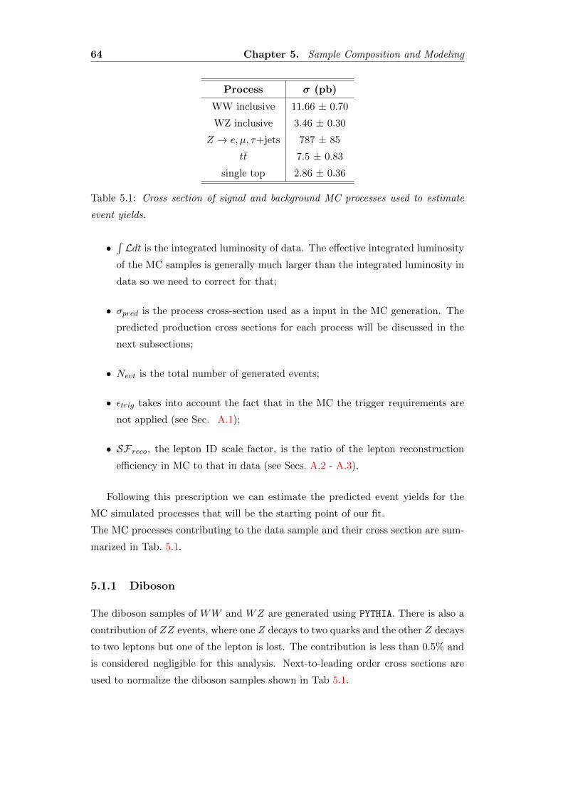
64 Chapter 5. Sample Composition and Modeling
Process σ (pb)
WW inclusive 11.66 ± 0.70
WZ inclusive 3.46 ± 0.30
Z → e, µ, τ+jets 787 ± 85
tt 7.5 ± 0.83
single top 2.86 ± 0.36
Table 5.1: Cross section of signal and background MC processes used to estimate
event yields.
•∫Ldt is the integrated luminosity of data. The effective integrated luminosity
of the MC samples is generally much larger than the integrated luminosity in
data so we need to correct for that;
• σpred is the process cross-section used as a input in the MC generation. The
predicted production cross sections for each process will be discussed in the
next subsections;
• Nevt is the total number of generated events;
• εtrig takes into account the fact that in the MC the trigger requirements are
not applied (see Sec. A.1);
• SFreco, the lepton ID scale factor, is the ratio of the lepton reconstruction
efficiency in MC to that in data (see Secs. A.2 - A.3).
Following this prescription we can estimate the predicted event yields for the
MC simulated processes that will be the starting point of our fit.
The MC processes contributing to the data sample and their cross section are sum-
marized in Tab. 5.1.
5.1.1 Diboson
The diboson samples of WW and WZ are generated using PYTHIA. There is also a
contribution of ZZ events, where one Z decays to two quarks and the other Z decays
to two leptons but one of the lepton is lost. The contribution is less than 0.5% and
is considered negligible for this analysis. Next-to-leading order cross sections are
used to normalize the diboson samples shown in Tab 5.1.
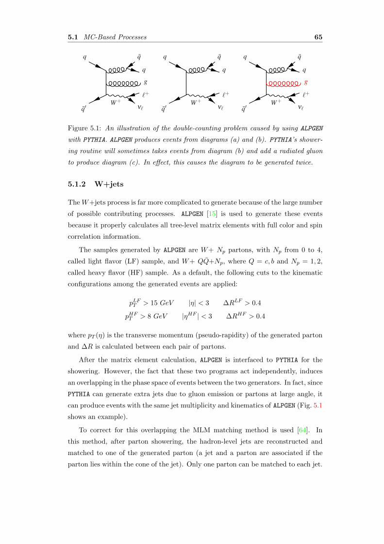
5.1 MC-Based Processes 65
W+
q′
q
νℓ
ℓ+
g
q
q
W+
q′
q
νℓ
ℓ+
q
q
W+
q′
q
νℓ
ℓ+
g
q
q
Figure 5.1: An illustration of the double-counting problem caused by using ALPGEN
with PYTHIA. ALPGEN produces events from diagrams (a) and (b). PYTHIA’s shower-
ing routine will sometimes takes events from diagram (b) and add a radiated gluon
to produce diagram (c). In effect, this causes the diagram to be generated twice.
5.1.2 W+jets
The W+jets process is far more complicated to generate because of the large number
of possible contributing processes. ALPGEN [15] is used to generate these events
because it properly calculates all tree-level matrix elements with full color and spin
correlation information.
The samples generated by ALPGEN are W+ Np partons, with Np from 0 to 4,
called light flavor (LF) sample, and W+ QQ+Np, where Q = c, b and Np = 1, 2,
called heavy flavor (HF) sample. As a default, the following cuts to the kinematic
configurations among the generated events are applied:
pLFT > 15 GeV |η| < 3 ∆RLF > 0.4
pHFT > 8 GeV |ηHF | < 3 ∆RHF > 0.4
where pT (η) is the transverse momentum (pseudo-rapidity) of the generated parton
and ∆R is calculated between each pair of partons.
After the matrix element calculation, ALPGEN is interfaced to PYTHIA for the
showering. However, the fact that these two programs act independently, induces
an overlapping in the phase space of events between the two generators. In fact, since
PYTHIA can generate extra jets due to gluon emission or partons at large angle, it
can produce events with the same jet multiplicity and kinematics of ALPGEN (Fig. 5.1
shows an example).
To correct for this overlapping the MLM matching method is used [64]. In
this method, after parton showering, the hadron-level jets are reconstructed and
matched to one of the generated parton (a jet and a parton are associated if the
parton lies within the cone of the jet). Only one parton can be matched to each jet.
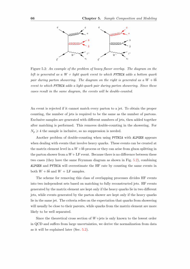
66 Chapter 5. Sample Composition and Modeling
W+
q′
q
νℓ
ℓ+
b
b
u
u
W+
q′
q
νℓ
ℓ+
b
b
u
u
Figure 5.2: An example of the problem of heavy flavor overlap. The diagram on the
left is generated as a W + light quark event to which PYTHIA adds a bottom quark
pair during parton showering. The diagram on the right is generated as a W + bb
event to which PYTHIA adds a light-quark pair during parton showering. Since these
cases result in the same diagram, the events will be double-counted.
An event is rejected if it cannot match every parton to a jet. To obtain the proper
counting, the number of jets is required to be the same as the number of partons.
Exclusive samples are generated with different numbers of jets, then added together
after matching is performed. This removes double-counting in the showering. For
Np > 4 the sample is inclusive, so no suppression is needed.
Another problem of double-counting when using PYTHIA with ALPGEN appears
when dealing with events that involve heavy quarks. These events can be created at
the matrix element level in a W+bb process or they can arise from gluon splitting in
the parton shower from aW+ LF event. Because there is no difference between these
two cases (they have the same Feynman diagram as shown in Fig. 5.2), combining
ALPGEN and PYTHIA will overestimate the HF rate by counting the same events in
both W + bb and W + LF samples.
The scheme for removing this class of overlapping processes divides HF events
into two independent sets based on matching to fully reconstructed jets. HF events
generated by the matrix element are kept only if the heavy quarks lie in two different
jets, while events generated by the parton shower are kept only if the heavy quarks
lie in the same jet. The criteria relies on the expectation that quarks from showering
will usually be close to their parents, while quarks from the matrix element are more
likely to be well separated.
Since the theoretical cross section of W+jets is only known to the lowest order
in QCD and suffers from large uncertainties, we derive the normalization from data
as it will be explained later (Sec. 5.2).
5.2 Data-Driven Background Modeling 67
5.1.3 Z+jets
As for the W+jets production, Z+jet is simulated using a combination of ALPGEN
matrix element generation and PYTHIA parton showering. In this case we use the
CDF inclusive Z + jets cross section measurement [65] for the normalization.
5.1.4 tt and single top production
tt production is simulated using PYTHIA. Single top events are generated using
MADEVENT again interfaced with PYTHIA for the showering. Both single top contri-
butions, s-channel and t-channel, are considered. We use their theoretical next-to-
leading order calculation [62] [63], assuming a top mass of 172.5 GeV/c2.
5.2 Data-Driven Background Modeling
One of the most challenging backgrounds to model is the QCD multijet one, where
a jet is faked by a lepton and mis-measurement of the jets energies leads to large
missing transverse energy. This effect is most relevant in the case of electrons, which
can be easily faked by jets of low track multiplicity and significant electromagnetic
energy1. This background is small relative to the dominant W+jets background,
but larger than the signal in electron events and roughly as large as the signal in
muon events. It is therefore important to correctly model its kinematics. Simulating
the QCD background is not feasible: the quite low rate for a jet to fake an electron
or a muon requires to generate huge QCD samples in order to have sufficient events
passing the event selection, and we need to be confident in the detector simulation.
Therefore, we choose to use data to model this background.
Since different lepton types may induce different rates and shapes of multijet
events, they need to be examined separately. This analysis uses two different models
for QCD events, one for electrons and one for muons. Both are based on the principle
that this process must contain a jet that is misidentified as a lepton. Thus, by
studying jets that are not leptons, but come close to passing leptons cuts, it is
possible to infer a model of this background.
For the muon sample we use non-isolated events, events which pass all selection’s
criteria except the requirement of lepton isolation. This is based on the rationale
that non-isolated leptons are typically leptons contained in jets, and jets that contain
1QCD multijet events can also contain real leptons from the decay of heavy flavor quarks, but
the background from fake leptons is larger.
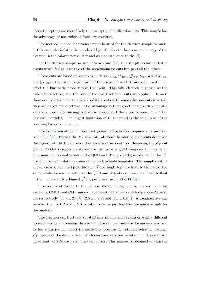
68 Chapter 5. Sample Composition and Modeling
energetic leptons are more likely to pass lepton identification cuts. This sample has
the advantage of not suffering from low statistics.
The method applied for muons cannot be used for the electron sample because,
in this case, the isolation is correlated by definition to the measured energy of the
electron in the calorimeter cluster and as a consequence to the ��ET .
For the electron sample we use anti-electrons [61]: this sample is constructed of
events which fail at least two of the non-kinematic cuts but pass all the others.
These cuts are based on variables, such as EHAD/EEM, χ2CES, Lshr, q×∆XCES,
and |∆zCES|, that are designed primarily to reject fake electrons but do not much
affect the kinematic properties of the event. This fake electron is chosen as the
candidate electron, and the rest of the event selection cuts are applied. Because
these events are similar to electrons data events with some selection cuts inverted,
they are called anti-electrons. The advantage is their good match with kinematic
variables, especially missing transverse energy and the angle between it and the
observed particles. The largest limitation of this method is the small size of the
resulting background sample;
The estimation of the multijet background normalization requires a data-driven
technique [66]. Fitting the ��ET is a natural choice because QCD events dominate
the region with little ��ET , since they have no true neutrino. Removing the ��ET cut
(��ET > 25 GeV) creates a data sample with a large QCD component. In order to
determine the normalization of the QCD and W+jets backgrounds, we fit the ��ET
distribution in the data to a sum of the backgrounds templates. The samples with a
known cross section (Z+jets, diboson, tt and single top) are fixed to their expected
value, while the normalization of the QCD and W+jets samples are allowed to float
in the fit. The fit is a binned χ2 fit, performed using MINUIT [67].
The results of the fit to the ��ET are shown in Fig. 5.3, separately for CEM
electrons, CMUP and CMX muons. The resulting fractions (with��ET above 25 GeV)
are respectively (10.7 ± 2.4)%, (2.5 ± 0.8)% and (3.1 ± 0.6)%. A weighted average
between the CMUP and CMX is taken once we put together the muon sample for
the analysis.
The fraction can fluctuate substantially in different regions or with a different
choice of histogram binning. In addition, the sample itself may be mis-modeled and
its low statistics may affect the sensitivity because the estimate relies on the high
��ET regime of the distribution, which can have very few events in it. A systematic
uncertainty of 25% covers all observed effects. This number is obtained varying the
5.3 Instantaneous Luminosity Correction 69
Met (GeV)0 50 100
Events
/4 G
eV
0
500
1000 /ndf = 36.43/242χ Data CMUP
Fit Result
W/Z+jet + Top + WW/WZ
QCD
QCD frac = 2.5
Met (GeV)0 50 100
Events
/4 G
eV
0
500
1000
1 = 4.30 fbL dt∫CDF Run II Preliminary
(a)
Met (GeV)0 50 100
Events
/4 G
eV
0
200
400
600 /ndf = 22.95/242χ Data CMX
Fit Result
W/Z+jet + Top + WW/WZ
QCD
QCD frac = 3.1
Met (GeV)0 50 100
Events
/4 G
eV
0
200
400
600
1 = 4.30 fbL dt∫CDF Run II Preliminary
(b)
Met (GeV)0 50 100
Events
/4 G
eV
0
1000
2000
3000
/ndf = 52.04/242χ
Data CEM
Fit Result
W/Z+jet + Top + WW/WZ
QCD
QCD frac = 10.7
Met (GeV)0 50 100
Events
/4 G
eV
0
1000
2000
3000
1 = 4.30 fbL dt∫CDF Run II Preliminary
(c)
Figure 5.3: Missing transverse energy fit of the QCD background for CMUP (a),
CMX (b) muons and CEM electrons (c). These fits refer to the offline selection
described in Chap. 4 with the ��ET cut released.
binning of the histograms and choosing different ranges of the fit.
A preliminary data-driven W+jets normalization is also derived from the fit to
the��ET distribution. This normalization is used in the modeling validation described
in Sec. 5.5. In the final fit for the extraction of the diboson cross section, the W+jets
normalization is a free parameter.
5.3 Instantaneous Luminosity Correction
Once the background levels are predicted, we want to investigate the agreement
between data and MC of various kinematic distributions. Before doing that, we

70 Chapter 5. Sample Composition and Modeling
need to apply another correction to the MC to take into account the different
luminosity profiles with respect to the data.
Different instantaneous luminosities can be simulated by tuning the number
of additional interactions per bunch crossing. The samples used in this analysis
were generated with two different luminosity profiles. The WW , WZ, and W+jets
samples have a profile based on the first 2.7 fb−1 of data recorded, while the other
samples were generated with a profile corresponding to the first 1 fb−1 of data.
Since we are using a 4.3 fb−1 data sample, and most of the additional data had
high instantaneous luminosities, we expect the average simulated instantaneous
luminosity to be lower than in our data sample.
A quantity directly related to the instantaneous luminosity is the number of
reconstructed vertices. The distribution of this quantity is shown in Fig. 5.4 with the
total MC prediction (stacked) overlayed. We deal with the observed disagreement
by re-weighting the MC events. Fig. 5.4 (bottom) shows the comparison of the
number of vertices in data and simulation after such re-weight.
5.4 Dijet Mass Shape
Once all the necessary ingredients to estimate the signal and the background are
described, we can directly compare the data with the MC expectations.
The first variable we are interested in is the invariant mass distribution of the
two leading jets, Mjj , shown in Fig 5.5. It is evident that the invariant mass shape
has a two peaks, where the second one starts around 40 GeV/c and extends above
our signal peak.
These peaks are kinematically correlated to the minimum jet energy require-
ment, the angular distance of the jets in the transverse plane (∆φ) and the combined
transverse momentum of the two jets (pT,jj) (shown in Fig. 5.6).
The requirement on the minimum jet energy of 20 GeV translates into two
different thresholds in the dijet invariant mass distribution, the first one, at Mjj ∼20 GeV/c2, is for almost collinear jets (∆φ ∼ 0.5), where the invariant mass is
minimum and the combined pT,jj is maximum. The second one is at Mjj ∼ 40
GeV/c2, for back to back jets (∆φ ∼ π), where the invariant mass is maximum.
The second threshold peak populates the region where the diboson peak is ex-
pected, in both distributions and this strongly reduces the signal sensitivity when
performing the fit. There are two possible choices to overcome this limitation:
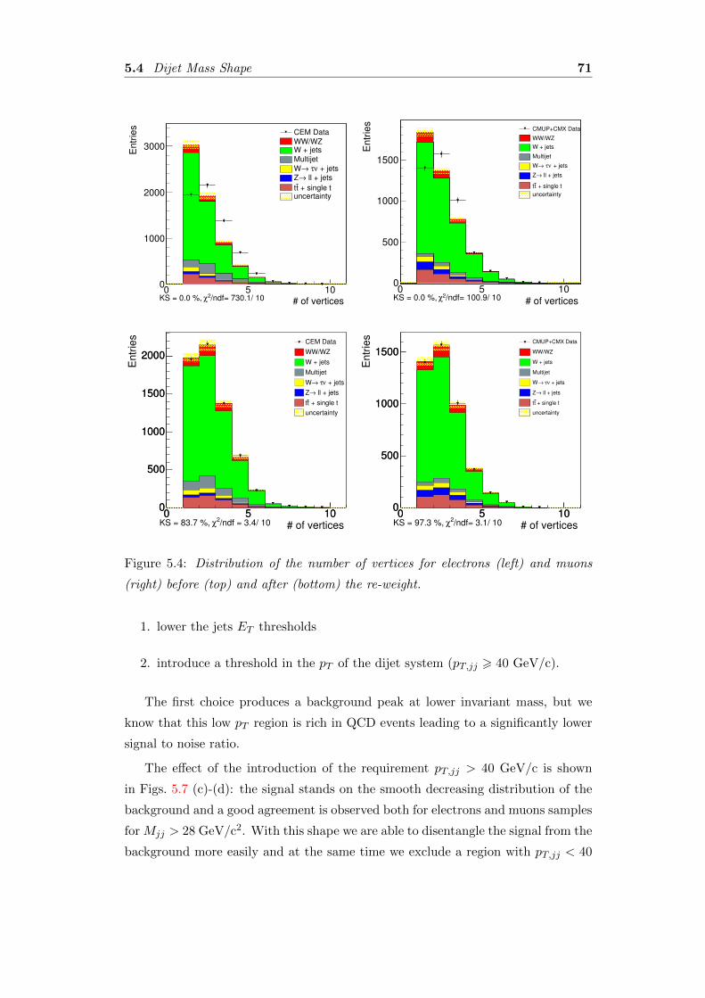
5.4 Dijet Mass Shape 71
# of vertices 0 5 10
En
trie
s
0
1000
2000
3000
/ndf= 730.1/ 10 2χKS = 0.0 %,
CEM Data
WW/WZW + jets
Multijet
+ jetsντ →W
ll + jets→Z
+ single tttuncertainty
# of vertices 0 5 10
Entr
ies
0
500
1000
1500
CMUP+CMX Data
WW/WZ
W + jets
Multijet
+ jetsντ →W
ll + jets→Z
+ single ttt
uncertainty
/ndf= 100.9/ 10 2χKS = 0.0 %,
# of vertices 0 5 10
Entr
ies
0
500
1000
1500
2000
0 5 100
500
1000
1500
2000
/ndf = 3.4/ 10 2χKS = 83.7 %,
CEM Data
WW/WZ
W + jets
Multijet
+ jetsντ →W
ll + jets→Z
+ single ttt
uncertainty
# of vertices 0 5 10
Entr
ies
0
500
1000
1500
0 5 100
500
1000
1500CMUP+CMX Data
WW/WZ
W + jets
Multijet
+ jetsντ →W
ll + jets→Z
+ single ttt
uncertainty
/ndf= 3.1/ 10 2χKS = 97.3 %,
Figure 5.4: Distribution of the number of vertices for electrons (left) and muons
(right) before (top) and after (bottom) the re-weight.
1. lower the jets ET thresholds
2. introduce a threshold in the pT of the dijet system (pT,jj > 40 GeV/c).
The first choice produces a background peak at lower invariant mass, but we
know that this low pT region is rich in QCD events leading to a significantly lower
signal to noise ratio.
The effect of the introduction of the requirement pT,jj > 40 GeV/c is shown
in Figs. 5.7 (c)-(d): the signal stands on the smooth decreasing distribution of the
background and a good agreement is observed both for electrons and muons samples
for Mjj > 28 GeV/c2. With this shape we are able to disentangle the signal from the
background more easily and at the same time we exclude a region with pT,jj < 40
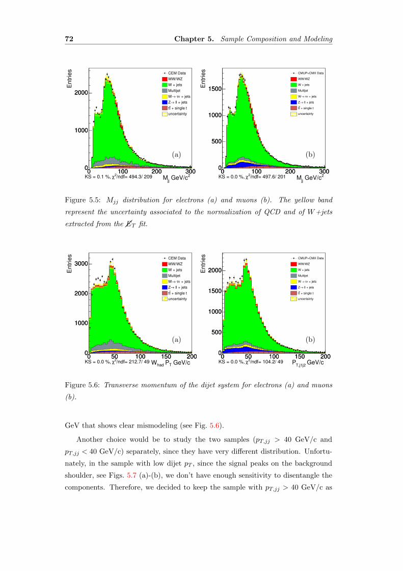
72 Chapter 5. Sample Composition and Modeling
2 GeV/cjj
M0 100 200 300
Entr
ies
0
1000
2000
0 100 200 3000
1000
2000
/ndf= 494.3/ 209 2χKS = 0.1 %,
CEM Data
WW/WZ
W + jets
Multijet
+ jetsντ →W
ll + jets→Z
+ single ttt
uncertainty
(a)
2 GeV/cjj
M0 100 200 300
Entr
ies
0
500
1000
1500
0 100 200 3000
500
1000
1500
CMUP+CMX Data
WW/WZ
W + jets
Multijet
+ jetsντ →W
ll + jets→Z
+ single ttt
uncertainty
/ndf= 497.6/ 201 2χKS = 0.0 %,
(b)
Figure 5.5: Mjj distribution for electrons (a) and muons (b). The yellow band
represent the uncertainty associated to the normalization of QCD and of W+jets
extracted from the ��ET fit.
GeV/c T PhadW0 50 100 150 200
Entr
ies
0
1000
2000
3000
0 50 100 150 2000
1000
2000
3000
/ndf= 212.7/ 49 2χKS = 0.0 %,
CEM Data
WW/WZ
W + jets
Multijet
+ jetsντ →W
ll + jets→Z
+ single ttt
uncertainty
(a)
GeV/c T,j1j2
P0 50 100 150 200
Entr
ies
0
500
1000
1500
2000
0 50 100 150 2000
500
1000
1500
2000
CMUP+CMX Data
WW/WZ
W + jets
Multijet
+ jetsντ →W
ll + jets→Z
+ single ttt
uncertainty
/ndf= 104.2/ 49 2χKS = 0.0 %,
(b)
Figure 5.6: Transverse momentum of the dijet system for electrons (a) and muons
(b).
GeV that shows clear mismodeling (see Fig. 5.6).
Another choice would be to study the two samples (pT,jj > 40 GeV/c and
pT,jj < 40 GeV/c) separately, since they have very different distribution. Unfortu-
nately, in the sample with low dijet pT , since the signal peaks on the background
shoulder, see Figs. 5.7 (a)-(b), we don’t have enough sensitivity to disentangle the
components. Therefore, we decided to keep the sample with pT,jj > 40 GeV/c as
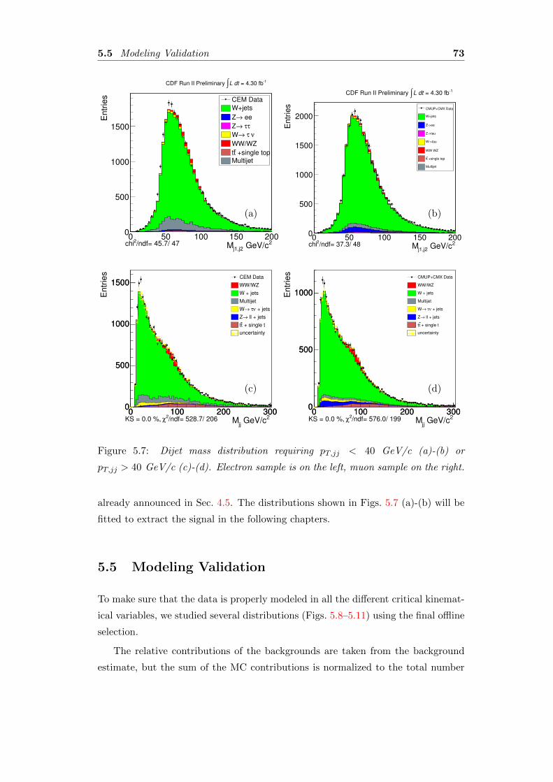
5.5 Modeling Validation 73
2 GeV/cj1,j2M0 50 100 150 200
En
trie
s
0
500
1000
1500
CEM Data
W+jets
ee→Z
ττ →Z
ν τ →W
WW/WZ
+single topttMultijet
/ndf= 45.7/ 47 2chi
1 = 4.30 fbL dt∫CDF Run II Preliminary
(a)
2 GeV/cj1,j2
M0 50 100 150 200
En
trie
s
0
500
1000
1500
2000CMUP+CMX Data
W+jets
Z>ee
Z>tau
W>tau
WW WZ
+single toptt
Multijet
/ndf= 37.3/ 48 2chi
1 = 4.30 fbL dt∫CDF Run II Preliminary
(b)
2 GeV/cjj
M0 100 200 300
Entr
ies
0
500
1000
1500
0 100 200 3000
500
1000
1500
/ndf= 528.7/ 206 2χKS = 0.0 %,
CEM Data
WW/WZ
W + jets
Multijet
+ jetsντ →W
ll + jets→Z
+ single ttt
uncertainty
(c)
2 GeV/cjj
M0 100 200 300
Entr
ies
0
500
1000
0 100 200 3000
500
1000
CMUP+CMX Data
WW/WZ
W + jets
Multijet
+ jetsντ →W
ll + jets→Z
+ single ttt
uncertainty
/ndf= 576.0/ 199 2χKS = 0.0 %,
(d)
Figure 5.7: Dijet mass distribution requiring pT,jj < 40 GeV/c (a)-(b) or
pT,jj > 40 GeV/c (c)-(d). Electron sample is on the left, muon sample on the right.
already announced in Sec. 4.5. The distributions shown in Figs. 5.7 (a)-(b) will be
fitted to extract the signal in the following chapters.
5.5 Modeling Validation
To make sure that the data is properly modeled in all the different critical kinemat-
ical variables, we studied several distributions (Figs. 5.8–5.11) using the final offline
selection.
The relative contributions of the backgrounds are taken from the background
estimate, but the sum of the MC contributions is normalized to the total number
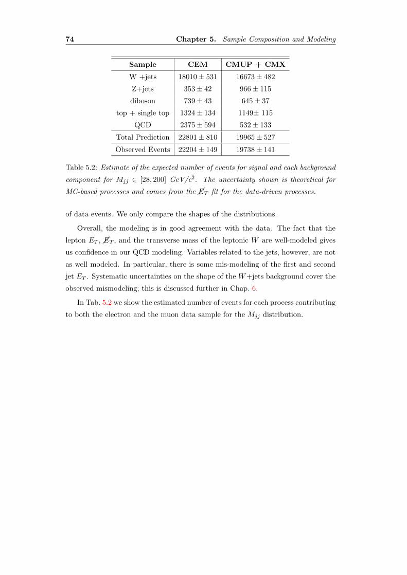
74 Chapter 5. Sample Composition and Modeling
Sample CEM CMUP + CMX
W +jets 18010± 531 16673± 482
Z+jets 353± 42 966± 115
diboson 739± 43 645± 37
top + single top 1324± 134 1149± 115
QCD 2375± 594 532± 133
Total Prediction 22801± 810 19965± 527
Observed Events 22204± 149 19738± 141
Table 5.2: Estimate of the expected number of events for signal and each background
component for Mjj ∈ [28, 200] GeV/c2. The uncertainty shown is theoretical for
MC-based processes and comes from the ��ET fit for the data-driven processes.
of data events. We only compare the shapes of the distributions.
Overall, the modeling is in good agreement with the data. The fact that the
lepton ET , ��ET , and the transverse mass of the leptonic W are well-modeled gives
us confidence in our QCD modeling. Variables related to the jets, however, are not
as well modeled. In particular, there is some mis-modeling of the first and second
jet ET . Systematic uncertainties on the shape of the W+jets background cover the
observed mismodeling; this is discussed further in Chap. 6.
In Tab. 5.2 we show the estimated number of events for each process contributing
to both the electron and the muon data sample for the Mjj distribution.
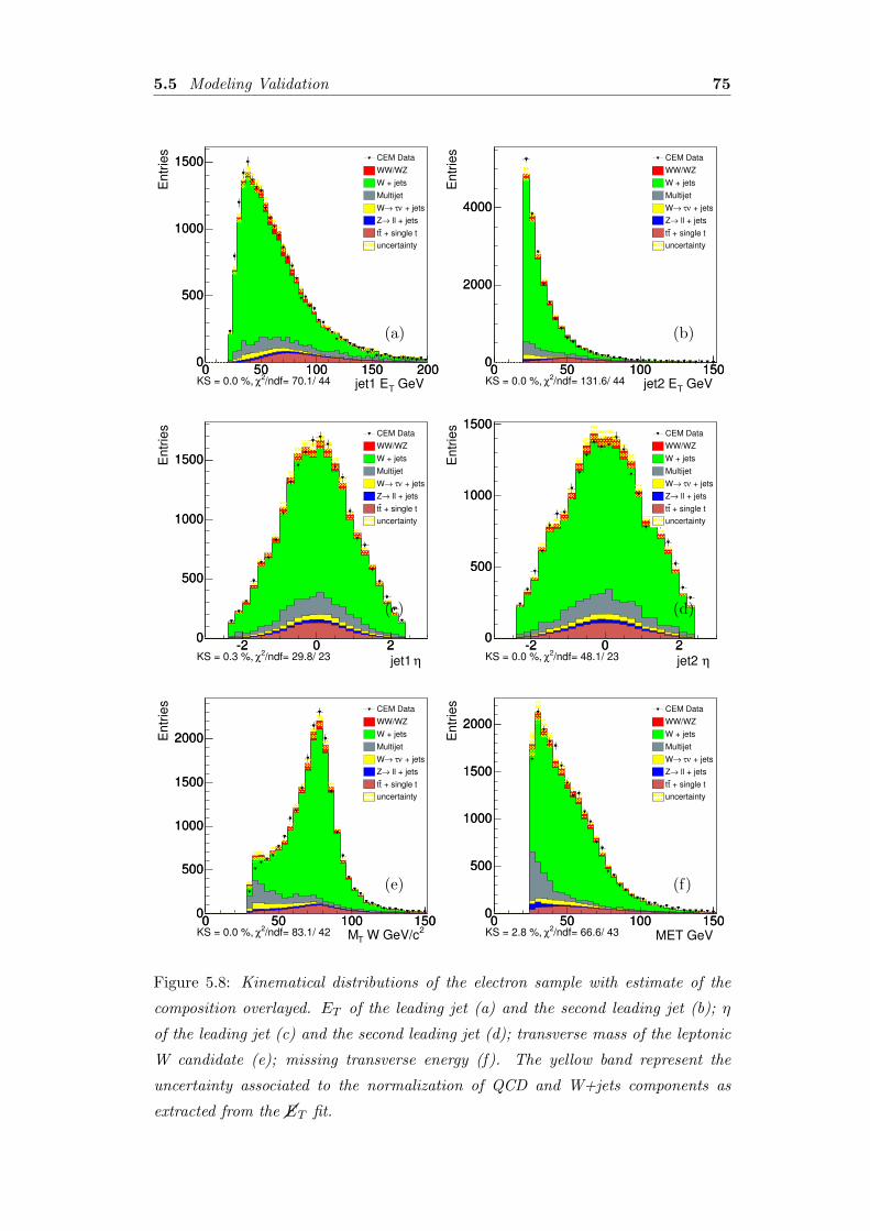
5.5 Modeling Validation 75
GeV Tjet1 E0 50 100 150 200
Entr
ies
0
500
1000
1500
0 50 100 150 2000
500
1000
1500
/ndf= 70.1/ 44 2χKS = 0.0 %,
CEM Data
WW/WZ
W + jets
Multijet
+ jetsντ →W
ll + jets→Z
+ single ttt
uncertainty
(a)
GeV Tjet2 E0 50 100 150
Entr
ies
0
2000
4000
0 50 100 1500
2000
4000
/ndf= 131.6/ 44 2χKS = 0.0 %,
CEM Data
WW/WZ
W + jets
Multijet
+ jetsντ →W
ll + jets→Z
+ single ttt
uncertainty
(b)
ηjet1 -2 0 2
Entr
ies
0
500
1000
1500
-2 0 20
500
1000
1500
/ndf= 29.8/ 23 2χKS = 0.3 %,
CEM Data
WW/WZ
W + jets
Multijet
+ jetsντ →W
ll + jets→Z
+ single ttt
uncertainty
(c)
ηjet2 -2 0 2
Entr
ies
0
500
1000
1500
-2 0 20
500
1000
1500
/ndf= 48.1/ 23 2χKS = 0.0 %,
CEM Data
WW/WZ
W + jets
Multijet
+ jetsντ →W
ll + jets→Z
+ single ttt
uncertainty
(d)
2 W GeV/cTM0 50 100 150
Entr
ies
0
500
1000
1500
2000
0 50 100 1500
500
1000
1500
2000
/ndf= 83.1/ 42 2χKS = 0.0 %,
CEM Data
WW/WZ
W + jets
Multijet
+ jetsντ →W
ll + jets→Z
+ single ttt
uncertainty
(e)
MET GeV 0 50 100 150
Entr
ies
0
500
1000
1500
2000
0 50 100 1500
500
1000
1500
2000
/ndf= 66.6/ 43 2χKS = 2.8 %,
CEM Data
WW/WZ
W + jets
Multijet
+ jetsντ →W
ll + jets→Z
+ single ttt
uncertainty
(f)
Figure 5.8: Kinematical distributions of the electron sample with estimate of the
composition overlayed. ET of the leading jet (a) and the second leading jet (b); η
of the leading jet (c) and the second leading jet (d); transverse mass of the leptonic
W candidate (e); missing transverse energy (f). The yellow band represent the
uncertainty associated to the normalization of QCD and W+jets components as
extracted from the ��ET fit.
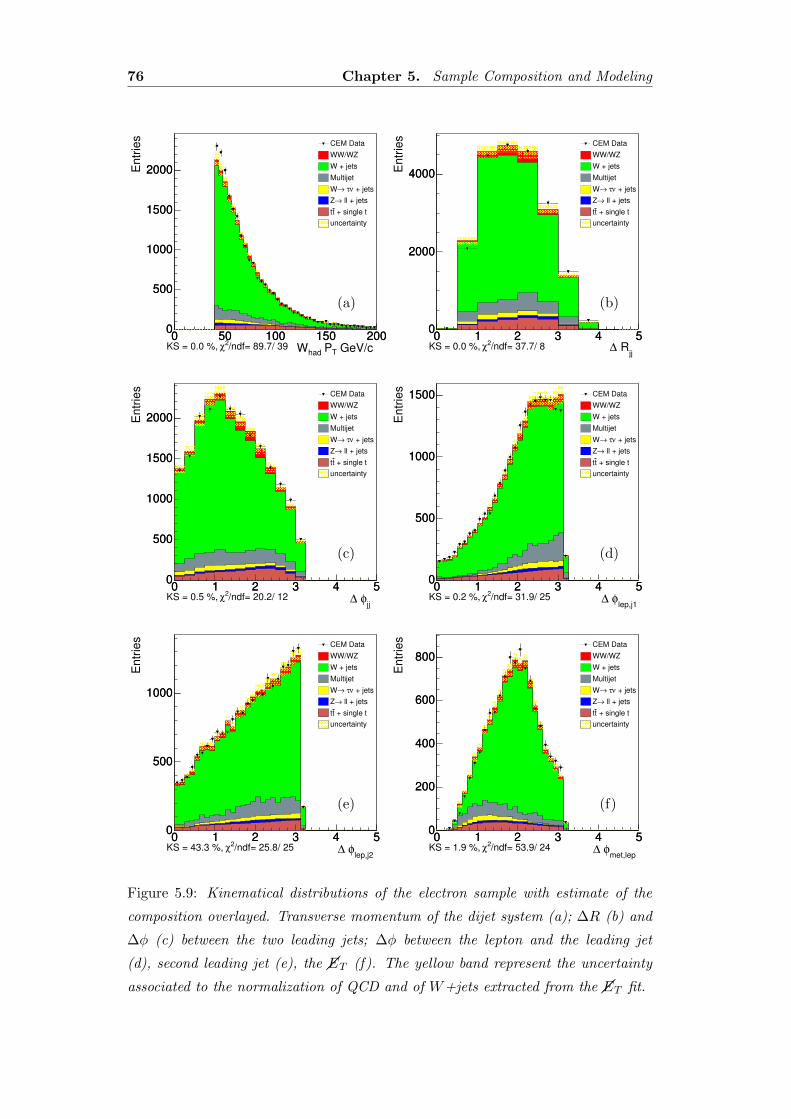
76 Chapter 5. Sample Composition and Modeling
GeV/c T PhadW0 50 100 150 200
Entr
ies
0
500
1000
1500
2000
0 50 100 150 2000
500
1000
1500
2000
/ndf= 89.7/ 39 2χKS = 0.0 %,
CEM Data
WW/WZ
W + jets
Multijet
+ jetsντ →W
ll + jets→Z
+ single ttt
uncertainty
(a)
jj
R∆0 1 2 3 4 5
Entr
ies
0
2000
4000
0 1 2 3 4 50
2000
4000
/ndf= 37.7/ 8 2χKS = 0.0 %,
CEM Data
WW/WZ
W + jets
Multijet
+ jetsντ →W
ll + jets→Z
+ single ttt
uncertainty
(b)
jj
φ ∆0 1 2 3 4 5
Entr
ies
0
500
1000
1500
2000
0 1 2 3 4 50
500
1000
1500
2000
/ndf= 20.2/ 12 2χKS = 0.5 %,
CEM Data
WW/WZ
W + jets
Multijet
+ jetsντ →W
ll + jets→Z
+ single ttt
uncertainty
(c)
lep,j1
φ ∆0 1 2 3 4 5
Entr
ies
0
500
1000
1500
0 1 2 3 4 50
500
1000
1500
/ndf= 31.9/ 25 2χKS = 0.2 %,
CEM Data
WW/WZ
W + jets
Multijet
+ jetsντ →W
ll + jets→Z
+ single ttt
uncertainty
(d)
lep,j2
φ ∆0 1 2 3 4 5
Entr
ies
0
500
1000
0 1 2 3 4 50
500
1000
/ndf= 25.8/ 25 2χKS = 43.3 %,
CEM Data
WW/WZ
W + jets
Multijet
+ jetsντ →W
ll + jets→Z
+ single ttt
uncertainty
(e)
met,lep
φ ∆0 1 2 3 4 5
Entr
ies
0
200
400
600
800
0 1 2 3 4 50
200
400
600
800
/ndf= 53.9/ 24 2χKS = 1.9 %,
CEM Data
WW/WZ
W + jets
Multijet
+ jetsντ →W
ll + jets→Z
+ single ttt
uncertainty
(f)
Figure 5.9: Kinematical distributions of the electron sample with estimate of the
composition overlayed. Transverse momentum of the dijet system (a); ∆R (b) and
∆φ (c) between the two leading jets; ∆φ between the lepton and the leading jet
(d), second leading jet (e), the ��ET (f). The yellow band represent the uncertainty
associated to the normalization of QCD and of W+jets extracted from the ��ET fit.
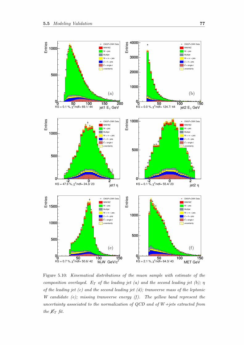
5.5 Modeling Validation 77
GeV Tjet1 E0 50 100 150 200
Entr
ies
0
500
1000
0 50 100 150 2000
500
1000
CMUP+CMX Data
WW/WZ
W + jets
Multijet
+ jetsντ →W
ll + jets→Z
+ single ttt
uncertainty
/ndf= 69.1/ 44 2χKS = 0.1 %,
(a)
GeV Tjet2 E0 50 100 150
Entr
ies
0
1000
2000
3000
4000
0 50 100 1500
1000
2000
3000
4000CMUP+CMX Data
WW/WZ
W + jets
Multijet
+ jetsντ →W
ll + jets→Z
+ single ttt
uncertainty
/ndf= 124.7/ 44 2χKS = 0.0 %,
(b)
ηjet1 -2 0 2
Entr
ies
0
500
1000
-2 0 20
500
1000
CMUP+CMX Data
WW/WZ
W + jets
Multijet
+ jetsντ →W
ll + jets→Z
+ single ttt
uncertainty
/ndf= 24.3/ 23 2χKS = 47.9 %,
(c)
ηjet2 -2 0 2
Entr
ies
0
500
1000
-2 0 20
500
1000 CMUP+CMX Data
WW/WZ
W + jets
Multijet
+ jetsντ →W
ll + jets→Z
+ single ttt
uncertainty
/ndf= 55.4/ 23 2χKS = 0.1 %,
(d)
2W GeV/cTM0 50 100 150
Entr
ies
0
500
1000
1500
0 50 100 1500
500
1000
1500
CMUP+CMX Data
WW/WZ
W + jets
Multijet
+ jetsντ →W
ll + jets→Z
+ single ttt
uncertainty
/ndf= 50.6/ 42 2χKS = 0.7 %,
(e)
MET GeV 0 50 100 150
Entr
ies
0
500
1000
0 50 100 1500
500
1000
CMUP+CMX Data
WW/WZ
W + jets
Multijet
+ jetsντ →W
ll + jets→Z
+ single ttt
uncertainty
/ndf= 64.3/ 43 2χKS = 2.1 %,
(f)
Figure 5.10: Kinematical distributions of the muon sample with estimate of the
composition overlayed. ET of the leading jet (a) and the second leading jet (b); η
of the leading jet (c) and the second leading jet (d); transverse mass of the leptonic
W candidate (e); missing transverse energy (f). The yellow band represent the
uncertainty associated to the normalization of QCD and of W+jets extracted from
the ��ET fit.

78 Chapter 5. Sample Composition and Modeling
GeV/c T,j1j2
P0 50 100 150 200
Entr
ies
0
500
1000
1500
0 50 100 150 2000
500
1000
1500
CMUP+CMX Data
WW/WZ
W + jets
Multijet
+ jetsντ →W
ll + jets→Z
+ single ttt
uncertainty
/ndf= 52.9/ 39 2χKS = 0.0 %,
(a)
jj
R∆0 1 2 3 4 5
Entr
ies
0
1000
2000
3000
0 1 2 3 4 50
1000
2000
3000
CMUP+CMX Data
WW/WZ
W + jets
Multijet
+ jetsντ →W
ll + jets→Z
+ single ttt
uncertainty
/ndf= 15.3/ 8 2χKS = 12.2 %,
(b)
jj
φ ∆0 1 2 3 4 5
Entr
ies
0
500
1000
1500
0 1 2 3 4 50
500
1000
1500
CMUP+CMX Data
WW/WZ
W + jets
Multijet
+ jetsντ →W
ll + jets→Z
+ single ttt
uncertainty
/ndf= 16.7/ 12 2χKS = 0.3 %,
(c)
lep,j1
φ ∆0 1 2 3 4 5
Entr
ies
0
500
1000
0 1 2 3 4 50
500
1000CMUP+CMX Data
WW/WZ
W + jets
Multijet
+ jetsντ →W
ll + jets→Z
+ single ttt
uncertainty
/ndf= 22.4/ 25 2χKS = 27.6 %,
(d)
lep,j2
φ ∆0 1 2 3 4 5
Entr
ies
0
500
1000
0 1 2 3 4 50
500
1000CMUP+CMX Data
WW/WZ
W + jets
Multijet
+ jetsντ →W
ll + jets→Z
+ single ttt
uncertainty
/ndf= 29.5/ 25 2χKS = 0.0 %,
(e)
lep,met
φ ∆0 1 2 3 4 5
Entr
ies
0
200
400
600
0 1 2 3 4 50
200
400
600 CMUP+CMX Data
WW/WZ
W + jets
Multijet
+ jetsντ →W
ll + jets→Z
+ single ttt
uncertainty
/ndf= 25.3/ 24 2χKS = 1.3 %,
(f)
Figure 5.11: Kinematical distributions of the muon sample with estimate of the
composition overlayed. Transverse momentum of the dijet system (a); ∆R (b) and
∆φ (c) between the two leading jets; ∆φ between the lepton and the leading jet
(d), second leading jet (e), the ��ET (f). The yellow band represent the uncertainty
associated to the normalization of QCD and of W+jets extracted from the ��ET fit.
Chapter 6
Fit Description and Validation
The technique used to extract the diboson contribution is a fit of the dijet mass
distribution to a linear combination of signal and backgrounds, whose modeling
has been described in the previous chapter. We now describe the fit procedure
and its validation through statistical trials. The following chapter will present its
application on the data.
6.1 Fit Procedure
Since the backgrounds contributing to the invariant mass distribution are not simply
parameterizable, we use directly the dijet mass “templates” (histograms normalized
to unit area), taken either from MC simulation or from data driven procedures, as
described in Chap. 5. With those we perform a binned χ2 fit to the data.
We perform the fit in each lepton channel separately, because the shapes and the
contributions of the backgrounds to the electron and the muon samples are different.
The fit parameters on each sample are: the total number of events and the fractions
of all components (signal and backgrounds) imposing that their total sum is equal to
1. The contributions of some backgrounds (QCD, tt + single top, Z+jets) are known
with a good theoretical or experimental precision, so we exploit this information to
increase the sensitivity in the determination of the signal fraction, by implementing
a Gaussian constraint on their fraction. The details about the templates, shown
in Figs. 6.1-6.2, and the fit parameters for the five components are outlined in the
following:
• WW/WZ: the dijet mass shapes are obtained combining the WW and WZ
templates, whose relative normalizations are fixed by MC after checking that
79
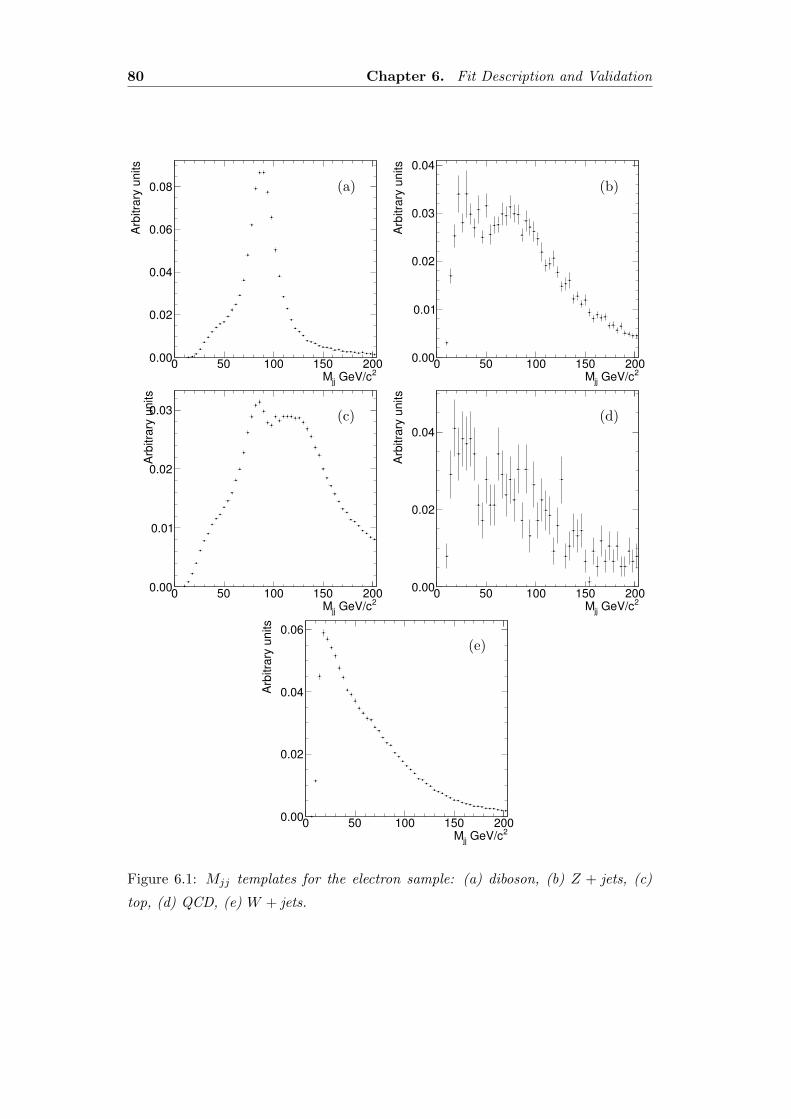
80 Chapter 6. Fit Description and Validation
2 GeV/cjjM0 50 100 150 200
Arb
itra
ry u
nits
0.00
0.02
0.04
0.06
0.08
1 = 4.30 fbL dt∫CDF Run II Preliminary
1 = 4.30 fbL dt∫CDF Run II Preliminary
(a)
2 GeV/cjjM0 50 100 150 200
Arb
itra
ry u
nits
0.00
0.01
0.02
0.03
0.04
1 = 4.30 fbL dt∫CDF Run II Preliminary
1 = 4.30 fbL dt∫CDF Run II Preliminary
(b)
2 GeV/cjjM0 50 100 150 200
Arb
itra
ry u
nits
0.00
0.01
0.02
0.03
1 = 4.30 fbL dt∫CDF Run II Preliminary
1 = 4.30 fbL dt∫CDF Run II Preliminary
(c)
2 GeV/cjjM0 50 100 150 200
Arb
itra
ry u
nits
0.00
0.02
0.04
1 = 4.30 fbL dt∫CDF Run II Preliminary
1 = 4.30 fbL dt∫CDF Run II Preliminary
(d)
2 GeV/cjjM0 50 100 150 200
Arb
itra
ry u
nits
0.00
0.02
0.04
0.06
1 = 4.30 fbL dt∫CDF Run II Preliminary
1 = 4.30 fbL dt∫CDF Run II Preliminary
(e)
Figure 6.1: Mjj templates for the electron sample: (a) diboson, (b) Z + jets, (c)
top, (d) QCD, (e) W + jets.
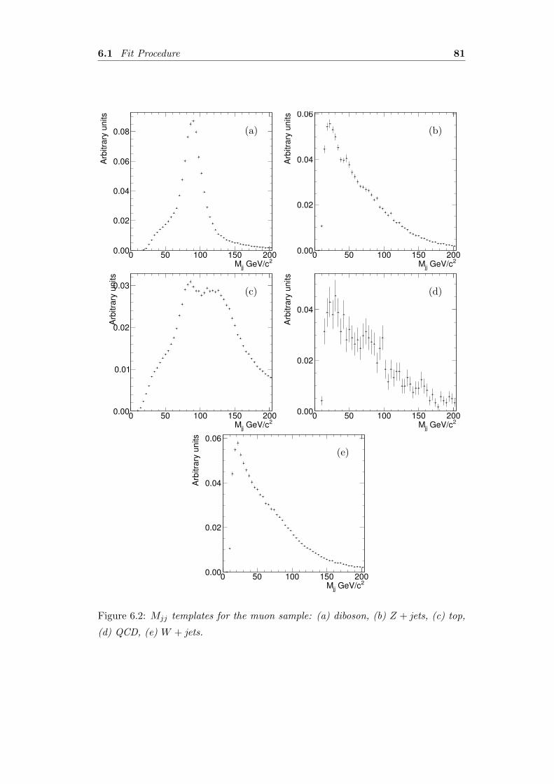
6.1 Fit Procedure 81
2 GeV/cjjM0 50 100 150 200
Arb
itra
ry u
nits
0.00
0.02
0.04
0.06
0.08
1 = 4.30 fbL dt∫CDF Run II Preliminary
1 = 4.30 fbL dt∫CDF Run II Preliminary
(a)
2 GeV/cjjM0 50 100 150 200
Arb
itra
ry u
nits
0.00
0.02
0.04
0.06
1 = 4.30 fbL dt∫CDF Run II Preliminary
1 = 4.30 fbL dt∫CDF Run II Preliminary
(b)
2 GeV/cjjM0 50 100 150 200
Arb
itra
ry u
nits
0.00
0.01
0.02
0.03
1 = 4.30 fbL dt∫CDF Run II Preliminary
1 = 4.30 fbL dt∫CDF Run II Preliminary
(c)
2 GeV/cjjM0 50 100 150 200
Arb
itra
ry u
nits
0.00
0.02
0.04
1 = 4.30 fbL dt∫CDF Run II Preliminary
1 = 4.30 fbL dt∫CDF Run II Preliminary
(d)
2 GeV/cjjM0 50 100 150 200
Arb
itra
ry u
nits
0.00
0.02
0.04
0.06
1 = 4.30 fbL dt∫CDF Run II Preliminary
1 = 4.30 fbL dt∫CDF Run II Preliminary
(e)
Figure 6.2: Mjj templates for the muon sample: (a) diboson, (b) Z + jets, (c) top,
(d) QCD, (e) W + jets.
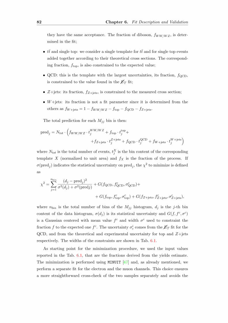
82 Chapter 6. Fit Description and Validation
they have the same acceptance. The fraction of diboson, fWW/WZ , is deter-
mined in the fit;
• tt and single top: we consider a single template for tt and for single top events
added together according to their theoretical cross sections. The correspond-
ing fraction, ftop, is also constrained to the expected value;
• QCD: this is the template with the largest uncertainties, its fraction, fQCD,
is constrained to the value found in the ��ET fit;
• Z+jets: its fraction, fZ+jets, is constrained to the measured cross section;
• W+jets: its fraction is not a fit parameter since it is determined from the
others as fW+jets = 1− fWW/WZ − ftop − fQCD − fZ+jets.
The total prediction for each Mjj bin is then:
predj = Ntot ·(fWW/WZ · tWW/WZ
j + ftop · ttopj +
+fZ+jets · tZ+jetsj + fQCD · tQCD
j + fW+jets · tW+jetsj
)where Ntot is the total number of events, tXj is the bin content of the corresponding
template X (normalized to unit area) and fX is the fraction of the process. If
σ(predj) indicates the statistical uncertainty on predj , the χ2 to minimize is defined
as
χ2 =
nbin∑j=1
(dj − predj)2
σ2(dj) + σ2(predj)+G(fQCD, f
cQCD, σ
cQCD)+
+G(ftop, fctop, σ
ctop) +G(fZ+jets, f
cZ+jets, σ
cZ+jets),
where nbin is the total number of bins of the Mjj histogram, dj is the j-th bin
content of the data histogram, σ(dj) is its statistical uncertainty and G(f, f c, σc)
is a Gaussian centered with mean value f c and width σc used to constraint the
fraction f to the expected one f c. The uncertainty σic comes from the ��ET fit for the
QCD, and from the theoretical and experimental uncertainty for top and Z+jets
respectively. The widths of the constraints are shown in Tab. 6.1.
As starting point for the minimization procedure, we used the input values
reported in the Tab. 6.1, that are the fractions derived from the yields estimate.
The minimization is performed using MINUIT [67] and, as already mentioned, we
perform a separate fit for the electron and the muon channels. This choice ensures
a more straightforward cross-check of the two samples separately and avoids the
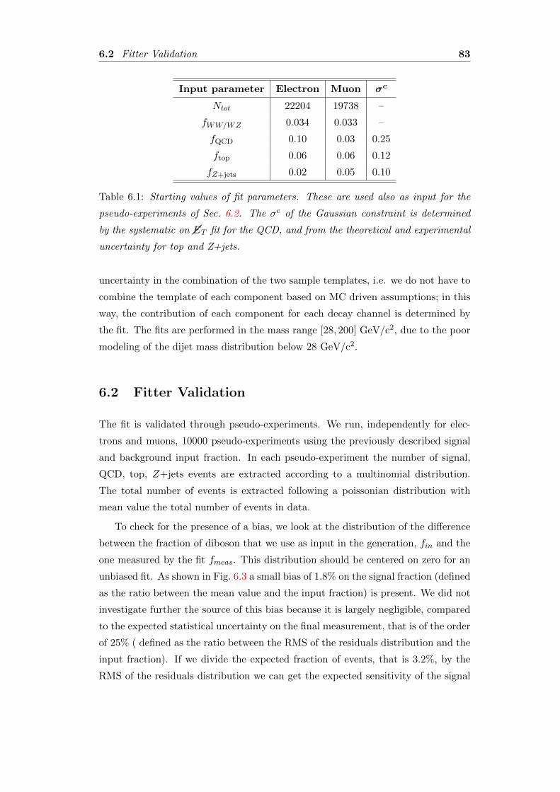
6.2 Fitter Validation 83
Input parameter Electron Muon σc
Ntot 22204 19738 –
fWW/WZ 0.034 0.033 –
fQCD 0.10 0.03 0.25
ftop 0.06 0.06 0.12
fZ+jets 0.02 0.05 0.10
Table 6.1: Starting values of fit parameters. These are used also as input for the
pseudo-experiments of Sec. 6.2. The σc of the Gaussian constraint is determined
by the systematic on ��ET fit for the QCD, and from the theoretical and experimental
uncertainty for top and Z+jets.
uncertainty in the combination of the two sample templates, i.e. we do not have to
combine the template of each component based on MC driven assumptions; in this
way, the contribution of each component for each decay channel is determined by
the fit. The fits are performed in the mass range [28, 200] GeV/c2, due to the poor
modeling of the dijet mass distribution below 28 GeV/c2.
6.2 Fitter Validation
The fit is validated through pseudo-experiments. We run, independently for elec-
trons and muons, 10000 pseudo-experiments using the previously described signal
and background input fraction. In each pseudo-experiment the number of signal,
QCD, top, Z+jets events are extracted according to a multinomial distribution.
The total number of events is extracted following a poissonian distribution with
mean value the total number of events in data.
To check for the presence of a bias, we look at the distribution of the difference
between the fraction of diboson that we use as input in the generation, fin and the
one measured by the fit fmeas. This distribution should be centered on zero for an
unbiased fit. As shown in Fig. 6.3 a small bias of 1.8% on the signal fraction (defined
as the ratio between the mean value and the input fraction) is present. We did not
investigate further the source of this bias because it is largely negligible, compared
to the expected statistical uncertainty on the final measurement, that is of the order
of 25% ( defined as the ratio between the RMS of the residuals distribution and the
input fraction). If we divide the expected fraction of events, that is 3.2%, by the
RMS of the residuals distribution we can get the expected sensitivity of the signal
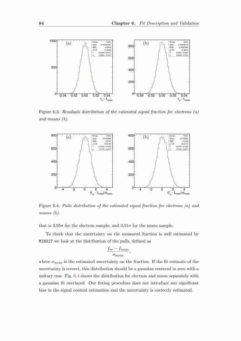
84 Chapter 6. Fit Description and Validation
meas fin
f
0.04 0.02 0.00 0.02 0.040
500
1000Entries 10000
Mean 0.000607287
RMS 0.00835
/ndf 2χ 31.23/29
µ 0.0001± 0.0006
σ 0.0001± 0.0084
(a)
meas fin
f
0.04 0.02 0.00 0.02 0.040
200
400
600
800
Entries 10000
Mean 0.000698719
RMS 0.00927296
/ndf 2χ 31.69/33
µ 0.0001± 0.0007
σ 0.0001± 0.0092
(b)
Figure 6.3: Residuals distribution of the estimated signal fraction for electrons (a)
and muons (b).
measσ)/meas fin
(f4 2 0 2 4
0
200
400
600
800 Entries 10000
Mean 0.0725866
RMS 1.02181
/ndf 2χ 37.60/36
µ 0.0102± 0.0748
σ 0.0071± 1.0173
(a)
measσ)/meas fin
(f4 2 0 2 4
0
200
400
600
800 Entries 10000
Mean 0.0728583
RMS 1.01604
/ndf 2χ 26.81/35
µ 0.0102± 0.0724
σ 0.0074± 1.0166
(b)
Figure 6.4: Pulls distribution of the estimated signal fraction for electrons (a) and
muons (b).
that is 3.95σ for the electron sample, and 3.51σ for the muon sample.
To check that the uncertainty on the measured fraction is well estimated by
MINUIT we look at the distribution of the pulls, defined as
fin − fmeasσmeas
,
where σmeas is the estimated uncertainty on the fraction. If the fit estimate of the
uncertainty is correct, this distribution should be a gaussian centered in zero with a
unitary rms. Fig. 6.4 shows the distribution for electron and muon separately with
a gaussian fit overlayed. Our fitting procedure does not introduce any significant
bias in the signal content estimation and the uncertainty is correctly estimated.
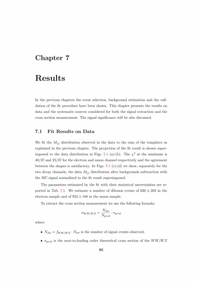
Chapter 7
Results
In the previous chapters the event selection, background estimation and the vali-
dation of the fit procedure have been shown. This chapter presents the results on
data and the systematic sources considered for both the signal extraction and the
cross section measurement. The signal significance will be also discussed.
7.1 Fit Results on Data
We fit the Mjj distribution observed in the data to the sum of the templates as
explained in the previous chapter. The projection of the fit result is shown super-
imposed to the data distribution in Figs. 7.1 (a)-(b). The χ2 at the minimum is
40/37 and 25/37 for the electron and muon channel respectively and the agreement
between the shapes is satisfactory. In Figs. 7.1 (c)-(d) we show, separately for the
two decay channels, the data Mjj distribution after backgrounds subtraction with
the MC signal normalized to the fit result superimposed.
The parameters estimated by the fit with their statistical uncertainties are re-
ported in Tab. 7.1. We estimate a number of diboson events of 630 ± 203 in the
electron sample and of 952± 188 in the muon sample.
To extract the cross section measurement we use the following formula:
σWW/WZ =Nobs
Npred· σpred
where
• Nobs = fWW/WZ ·Ntot is the number of signal events observed;
• σpred is the next-to-leading order theoretical cross section of the WW/WZ
85
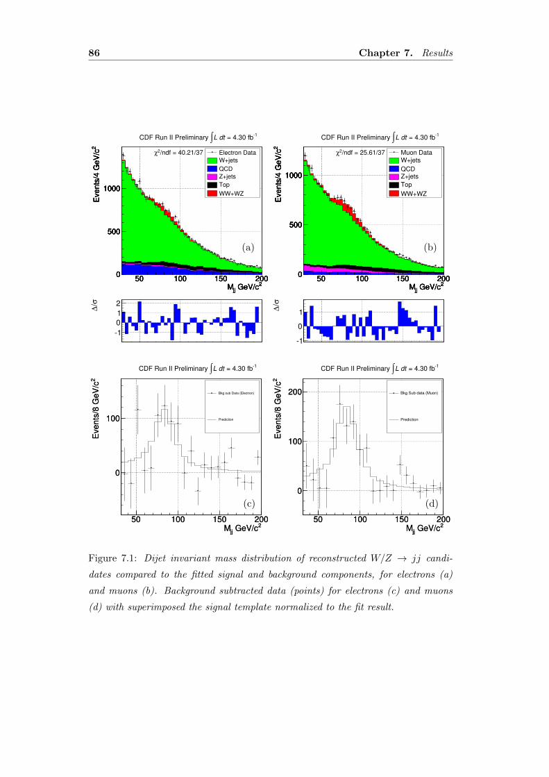
86 Chapter 7. Results
2 GeV/cjjM
50 100 150 200
2E
ve
nts
/4 G
eV
/c
0
500
1000
/ndf = 40.21/372χ Electron Data
W+jets
QCD
Z+jets
Top
WW+WZ
2 GeV/cjjM
50 100 150 200
2E
ve
nts
/4 G
eV
/c
0
500
1000
1 = 4.30 fbL dt∫CDF Run II Preliminary
2 GeV/cjjM
50 100 150 200
2E
ve
nts
/4 G
eV
/c
0
500
1000
2 GeV/cjjM
50 100 150 200
2E
ve
nts
/4 G
eV
/c
0
500
1000
σ/∆
1
0
1
2
(a)
2 GeV/cjjM
50 100 150 2002
Eve
nts
/4 G
eV
/c0
500
1000
/ndf = 25.61/372χ Muon DataW+jets
QCDZ+jets
Top
WW+WZ
2 GeV/cjjM
50 100 150 2002
Eve
nts
/4 G
eV
/c0
500
1000
1 = 4.30 fbL dt∫CDF Run II Preliminary
2 GeV/cjjM
50 100 150 2002
Eve
nts
/4 G
eV
/c0
500
1000
2 GeV/cjjM
50 100 150 2002
Eve
nts
/4 G
eV
/c0
500
1000
σ/∆
1
0
1
(b)
2 GeV/cjjM50 100 150 200
2E
vents
/8 G
eV
/c
0
100
Bkg sub Data (Electron)
Prediction
2 GeV/cjjM50 100 150 200
2E
vents
/8 G
eV
/c
0
100
1 = 4.30 fbL dt∫CDF Run II Preliminary
(c)
2 GeV/cjjM50 100 150 200
2E
vents
/8 G
eV
/c
0
100
200 Bkg Sub data (Muon)
Prediction
2 GeV/cjjM50 100 150 200
2E
vents
/8 G
eV
/c
0
100
200
1 = 4.30 fbL dt∫CDF Run II Preliminary
(d)
Figure 7.1: Dijet invariant mass distribution of reconstructed W/Z → jj candi-
dates compared to the fitted signal and background components, for electrons (a)
and muons (b). Background subtracted data (points) for electrons (c) and muons
(d) with superimposed the signal template normalized to the fit result.
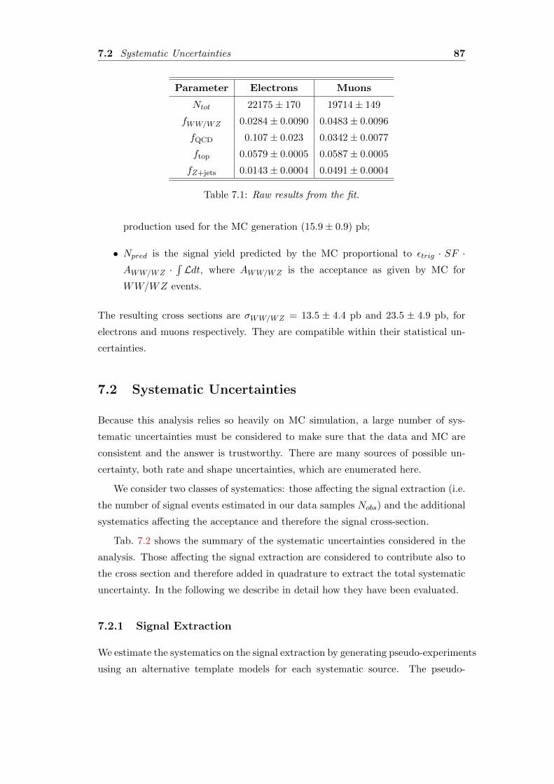
7.2 Systematic Uncertainties 87
Parameter Electrons Muons
Ntot 22175± 170 19714± 149
fWW/WZ 0.0284± 0.0090 0.0483± 0.0096
fQCD 0.107± 0.023 0.0342± 0.0077
ftop 0.0579± 0.0005 0.0587± 0.0005
fZ+jets 0.0143± 0.0004 0.0491± 0.0004
Table 7.1: Raw results from the fit.
production used for the MC generation (15.9± 0.9) pb;
• Npred is the signal yield predicted by the MC proportional to εtrig · SF ·AWW/WZ ·
∫Ldt, where AWW/WZ is the acceptance as given by MC for
WW/WZ events.
The resulting cross sections are σWW/WZ = 13.5 ± 4.4 pb and 23.5 ± 4.9 pb, for
electrons and muons respectively. They are compatible within their statistical un-
certainties.
7.2 Systematic Uncertainties
Because this analysis relies so heavily on MC simulation, a large number of sys-
tematic uncertainties must be considered to make sure that the data and MC are
consistent and the answer is trustworthy. There are many sources of possible un-
certainty, both rate and shape uncertainties, which are enumerated here.
We consider two classes of systematics: those affecting the signal extraction (i.e.
the number of signal events estimated in our data samples Nobs) and the additional
systematics affecting the acceptance and therefore the signal cross-section.
Tab. 7.2 shows the summary of the systematic uncertainties considered in the
analysis. Those affecting the signal extraction are considered to contribute also to
the cross section and therefore added in quadrature to extract the total systematic
uncertainty. In the following we describe in detail how they have been evaluated.
7.2.1 Signal Extraction
We estimate the systematics on the signal extraction by generating pseudo-experiments
using an alternative template models for each systematic source. The pseudo-
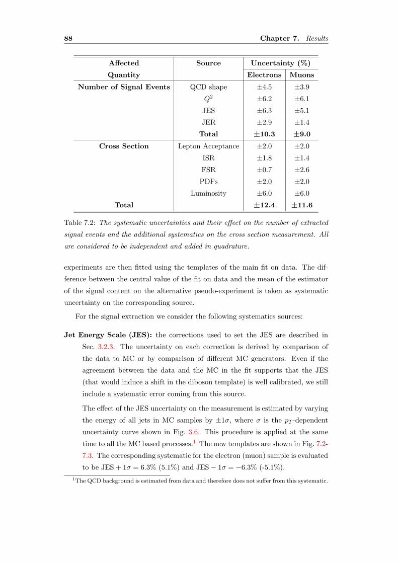
88 Chapter 7. Results
Affected Source Uncertainty (%)
Quantity Electrons Muons
Number of Signal Events QCD shape ±4.5 ±3.9
Q2 ±6.2 ±6.1
JES ±6.3 ±5.1
JER ±2.9 ±1.4
Total ±10.3 ±9.0
Cross Section Lepton Acceptance ±2.0 ±2.0
ISR ±1.8 ±1.4
FSR ±0.7 ±2.6
PDFs ±2.0 ±2.0
Luminosity ±6.0 ±6.0
Total ±12.4 ±11.6
Table 7.2: The systematic uncertainties and their effect on the number of extracted
signal events and the additional systematics on the cross section measurement. All
are considered to be independent and added in quadrature.
experiments are then fitted using the templates of the main fit on data. The dif-
ference between the central value of the fit on data and the mean of the estimator
of the signal content on the alternative pseudo-experiment is taken as systematic
uncertainty on the corresponding source.
For the signal extraction we consider the following systematics sources:
Jet Energy Scale (JES): the corrections used to set the JES are described in
Sec. 3.2.3. The uncertainty on each correction is derived by comparison of
the data to MC or by comparison of different MC generators. Even if the
agreement between the data and the MC in the fit supports that the JES
(that would induce a shift in the diboson template) is well calibrated, we still
include a systematic error coming from this source.
The effect of the JES uncertainty on the measurement is estimated by varying
the energy of all jets in MC samples by ±1σ, where σ is the pT -dependent
uncertainty curve shown in Fig. 3.6. This procedure is applied at the same
time to all the MC based processes.1 The new templates are shown in Fig. 7.2-
7.3. The corresponding systematic for the electron (muon) sample is evaluated
to be JES + 1σ = 6.3% (5.1%) and JES− 1σ = −6.3% (-5.1%).
1The QCD background is estimated from data and therefore does not suffer from this systematic.
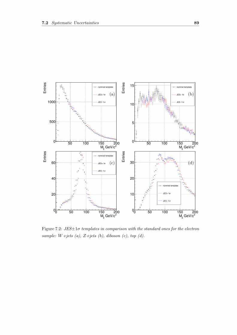
7.2 Systematic Uncertainties 89
2 GeV/cjjM50 100 150 200
Entr
ies
0
500
1000
1 = 4.30 fbL dt∫CDF Run II Preliminary
nominal template
σJES+ 1
σJES 1
nominal template
σJES+ 1
σJES 1
(a)
2 GeV/cjjM50 100 150 200
Entr
ies
0
5
10
15
1 = 4.30 fbL dt∫CDF Run II Preliminary
nominal template
σJES+ 1
σJES 1
nominal template
σJES+ 1
σJES 1
(b)
2 GeV/cjjM0 50 100 150 200
Entr
ies
0
20
40
60
1 = 4.30 fbL dt∫CDF Run II Preliminary
nominal template
σJES+ 1
σJES 1
nominal template
σJES+ 1
σJES 1
(c)
2 GeV/cjjM0 50 100 150 200
Entr
ies
0
10
20
30
1 = 4.30 fbL dt∫CDF Run II Preliminary
nominal template
σJES+ 1
σJES 1
nominal template
σJES+ 1
σJES 1
(d)
Figure 7.2: JES±1σ templates in comparison with the standard ones for the electron
sample: W+jets (a), Z+jets (b), diboson (c), top (d).
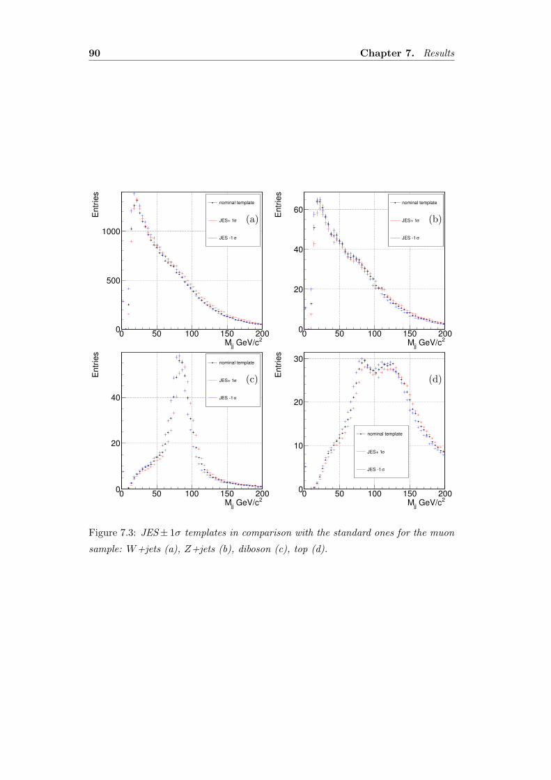
90 Chapter 7. Results
2 GeV/cjjM0 50 100 150 200
Entr
ies
0
500
1000
1 = 4.30 fbL dt∫CDF Run II Preliminary
nominal template
σJES+ 1
σJES 1
nominal template
σJES+ 1
σJES 1
(a)
2 GeV/cjjM0 50 100 150 200
Entr
ies
0
20
40
60
1 = 4.30 fbL dt∫CDF Run II Preliminary
nominal template
σJES+ 1
σJES 1
nominal template
σJES+ 1
σJES 1
(b)
2 GeV/cjjM0 50 100 150 200
Entr
ies
0
20
40
1 = 4.30 fbL dt∫CDF Run II Preliminary
nominal template
σJES+ 1
σJES 1
nominal template
σJES+ 1
σJES 1
(c)
2 GeV/cjjM0 50 100 150 200
Entr
ies
0
10
20
30
1 = 4.30 fbL dt∫CDF Run II Preliminary
nominal template
σJES+ 1
σJES 1
nominal template
σJES+ 1
σJES 1
(d)
Figure 7.3: JES± 1σ templates in comparison with the standard ones for the muon
sample: W+jets (a), Z+jets (b), diboson (c), top (d).
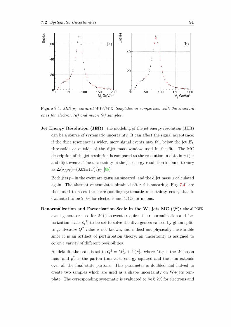
7.2 Systematic Uncertainties 91
2 GeV/cjjM0 50 100 150 200
Entr
ies
0
20
40
60
1 = 4.30 fbL dt∫CDF Run II Preliminary
(a)
2 GeV/cjjM0 50 100 150 200
Entr
ies
0
20
40
1 = 4.30 fbL dt∫CDF Run II Preliminary
(b)
Figure 7.4: JER pT smeared WW/WZ templates in comparison with the standard
ones for electron (a) and muon (b) samples.
Jet Energy Resolution (JER): the modeling of the jet energy resolution (JER)
can be a source of systematic uncertainty. It can affect the signal acceptance:
if the dijet resonance is wider, more signal events may fall below the jet ET
thresholds or outside of the dijet mass window used in the fit. The MC
description of the jet resolution is compared to the resolution in data in γ+jet
and dijet events. The uncertainty in the jet energy resolution is found to vary
as ∆(σ/pT )=(0.03±1.7)/pT [68].
Both jets pT in the event are gaussian smeared, and the dijet mass is calculated
again. The alternative templates obtained after this smearing (Fig. 7.4) are
then used to asses the corresponding systematic uncertainty error, that is
evaluated to be 2.9% for electrons and 1.4% for muons.
Renormalization and Factorization Scale in the W+jets MC (Q2): the ALPGEN
event generator used for W+jets events requires the renormalization and fac-
torization scale, Q2, to be set to solve the divergences caused by gluon split-
ting. Because Q2 value is not known, and indeed not physically measurable
since it is an artifact of perturbation theory, an uncertainty is assigned to
cover a variety of different possibilities.
As default, the scale is set to Q2 = M2W +
∑p2T , where MW is the W boson
mass and p2T is the parton transverse energy squared and the sum extends
over all the final state partons. This parameter is doubled and halved to
create two samples which are used as a shape uncertainty on W+jets tem-
plate. The corresponding systematic is evaluated to be 6.2% for electrons and
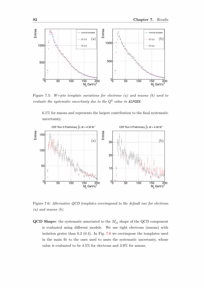
92 Chapter 7. Results
2 GeV/cjjM0 50 100 150 200
Entr
ies
0
500
1000
1 = 4.30 fbL dt∫CDF Run II Preliminary
nominal template
=2.02
Q
=0.52
Q
nominal template
=2.02
Q
=0.52
Q
(a)
2 GeV/cjjM0 50 100 150 200
Entr
ies
0
500
1000
1 = 4.30 fbL dt∫CDF Run II Preliminary
nominal template
=2.02
Q
=0.52
Q
nominal template
=2.02
Q
=0.52
Q
(b)
Figure 7.5: W+jets template variations for electrons (a) and muons (b) used to
evaluate the systematic uncertanty due to the Q2 value in ALPGEN.
6.1% for muons and represents the largest contribution to the final systematic
uncertainty.
2 GeV/cjjM0 50 100 150 200
Entr
ies
0
50
100
150
1 = 4.30 fbL dt∫CDF Run II Preliminary
(a)
2 GeV/cjjM0 50 100 150 200
Entr
ies
0
10
20
30
1 = 4.30 fbL dt∫CDF Run II Preliminary
(b)
Figure 7.6: Alternative QCD templates overimposed to the default one for electrons
(a) and muons (b).
QCD Shape: the systematic associated to the Mjj shape of the QCD component
is evaluated using different models. We use tight electrons (muons) with
isolation grater than 0.2 (0.4). In Fig. 7.6 we overimpose the templates used
in the main fit to the ones used to asses the systematic uncertanty, whose
value is evaluated to be 4.5% for electrons and 3.9% for muons.
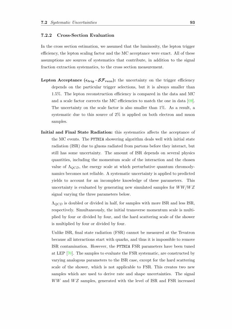
7.2 Systematic Uncertainties 93
7.2.2 Cross-Section Evaluation
In the cross section estimation, we assumed that the luminosity, the lepton trigger
efficiency, the lepton scaling factor and the MC acceptance were exact. All of these
assumptions are sources of systematics that contribute, in addition to the signal
fraction extraction systematics, to the cross section measurement.
Lepton Acceptance (εtrig · SFreco): the uncertainty on the trigger efficiency
depends on the particular trigger selections, but it is always smaller than
1.5%. The lepton reconstruction efficiency is compared in the data and MC
and a scale factor corrects the MC efficiencies to match the one in data [69].
The uncertainty on the scale factor is also smaller than 1%. As a result, a
systematic due to this source of 2% is applied on both electron and muon
samples.
Initial and Final State Radiation: this systematics affects the acceptance of
the MC events. The PYTHIA showering algorithm deals well with initial state
radiation (ISR) due to gluons radiated from partons before they interact, but
still has some uncertainty. The amount of ISR depends on several physics
quantities, including the momentum scale of the interaction and the chosen
value of ΛQCD, the energy scale at which perturbative quantum chromody-
namics becomes not reliable. A systematic uncertainty is applied to predicted
yields to account for an incomplete knowledge of these parameters. This
uncertainty is evaluated by generating new simulated samples for WW/WZ
signal varying the three parameters below.
ΛQCD is doubled or divided in half, for samples with more ISR and less ISR,
respectively. Simultaneously, the initial transverse momentum scale is multi-
plied by four or divided by four, and the hard scattering scale of the shower
is multiplied by four or divided by four.
Unlike ISR, final state radiation (FSR) cannot be measured at the Tevatron
because all interactions start with quarks, and thus it is impossible to remove
ISR contamination. However, the PYTHIA FSR parameters have been tuned
at LEP [70]. The samples to evaluate the FSR systematic, are constructed by
varying analogous parameters to the ISR case, except for the hard scattering
scale of the shower, which is not applicable to FSR. This creates two new
samples which are used to derive rate and shape uncertainties. The signal
WW and WZ samples, generated with the level of ISR and FSR increased
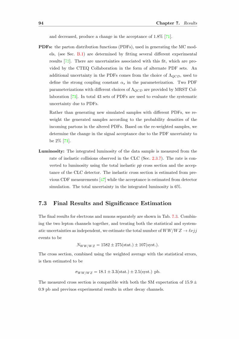
94 Chapter 7. Results
and decreased, produce a change in the acceptance of 1.8% [71].
PDFs: the parton distribution functions (PDFs), used in generating the MC mod-
els, (see Sec. B.1) are determined by fitting several different experimental
results [72]. There are uncertainties associated with this fit, which are pro-
vided by the CTEQ Collaboration in the form of alternate PDF sets. An
additional uncertainty in the PDFs comes from the choice of ΛQCD, used to
define the strong coupling constant αs in the parameterization. Two PDF
parameterizations with different choices of ΛQCD are provided by MRST Col-
laboration [73]. In total 43 sets of PDFs are used to evaluate the systematic
uncertainty due to PDFs.
Rather than generating new simulated samples with different PDFs, we re-
weight the generated samples according to the probability densities of the
incoming partons in the altered PDFs. Based on the re-weighted samples, we
determine the change in the signal acceptance due to the PDF uncertainty to
be 2% [71].
Luminosity: The integrated luminosity of the data sample is measured from the
rate of inelastic collisions observed in the CLC (Sec. 2.3.7). The rate is con-
verted to luminosity using the total inelastic pp cross section and the accep-
tance of the CLC detector. The inelastic cross section is estimated from pre-
vious CDF measurements [47] while the acceptance is estimated from detector
simulation. The total uncertainty in the integrated luminosity is 6%.
7.3 Final Results and Significance Estimation
The final results for electrons and muons separately are shown in Tab. 7.3. Combin-
ing the two lepton channels together, and treating both the statistical and system-
atic uncertainties as independent, we estimate the total number ofWW/WZ → `νjj
events to be
NWW/WZ = 1582± 275(stat.)± 107(syst.).
The cross section, combined using the weighted average with the statistical errors,
is then estimated to be
σWW/WZ = 18.1± 3.3(stat.)± 2.5(syst.) pb.
The measured cross section is compatible with both the SM expectation of 15.9 ±0.9 pb and previuos experimental results in other decay channels.
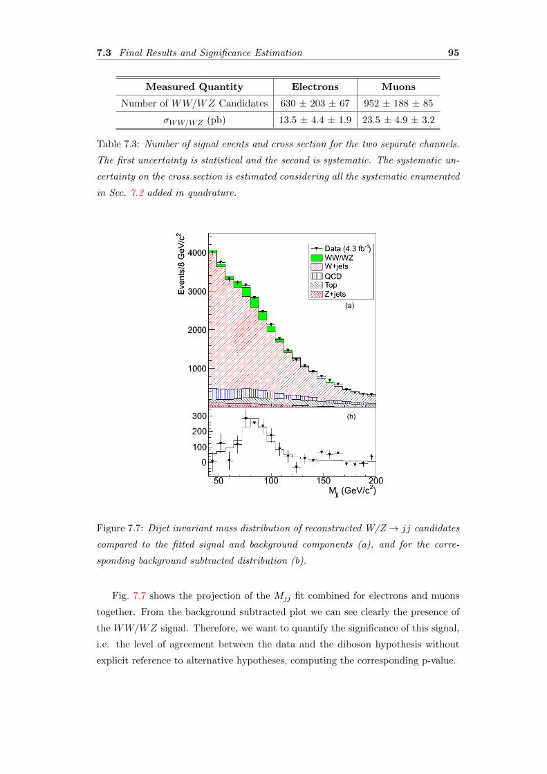
7.3 Final Results and Significance Estimation 95
Measured Quantity Electrons Muons
Number of WW/WZ Candidates 630 ± 203 ± 67 952 ± 188 ± 85
σWW/WZ (pb) 13.5 ± 4.4 ± 1.9 23.5 ± 4.9 ± 3.2
Table 7.3: Number of signal events and cross section for the two separate channels.
The first uncertainty is statistical and the second is systematic. The systematic un-
certainty on the cross section is estimated considering all the systematic enumerated
in Sec. 7.2 added in quadrature.
Figure 7.7: Dijet invariant mass distribution of reconstructed W/Z → jj candidates
compared to the fitted signal and background components (a), and for the corre-
sponding background subtracted distribution (b).
Fig. 7.7 shows the projection of the Mjj fit combined for electrons and muons
together. From the background subtracted plot we can see clearly the presence of
the WW/WZ signal. Therefore, we want to quantify the significance of this signal,
i.e. the level of agreement between the data and the diboson hypothesis without
explicit reference to alternative hypotheses, computing the corresponding p-value.
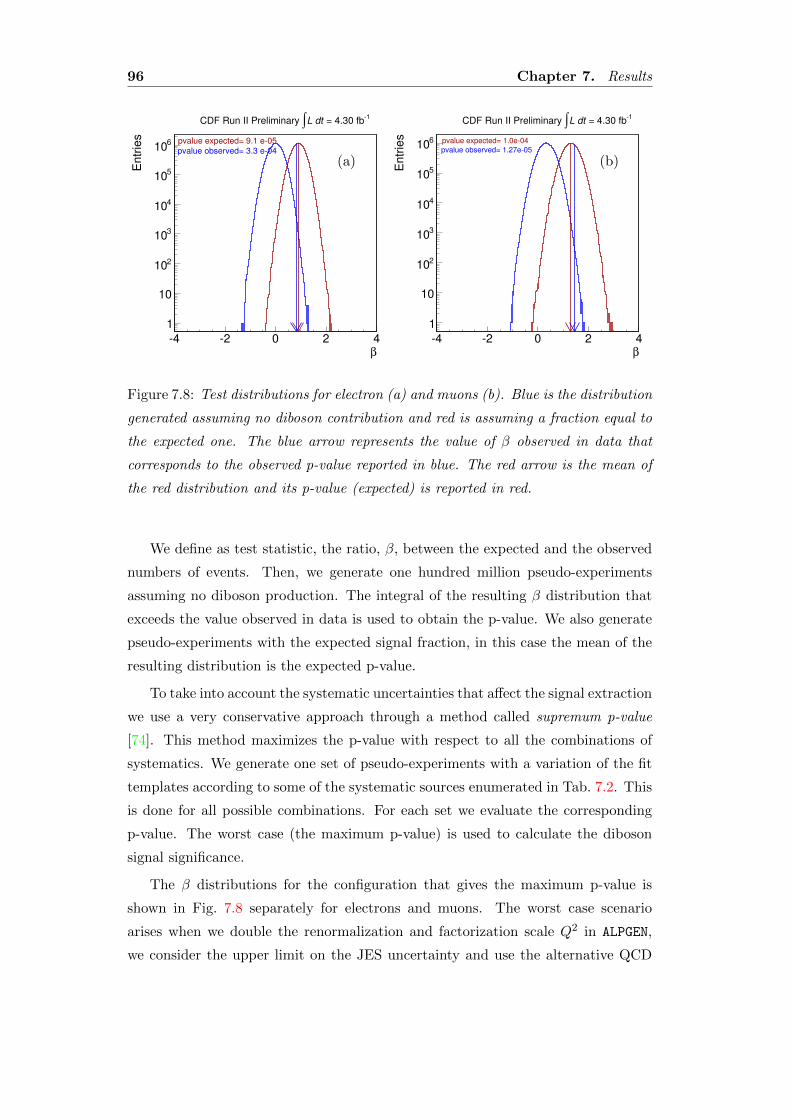
96 Chapter 7. Results
β4 2 0 2 4
Entr
ies
1
10
210
310
410
510
610 pvalue observed= 3.3 e04
pvalue expected= 9.1 e05
1 = 4.30 fbL dt∫CDF Run II Preliminary
(a)
β4 2 0 2 4
Entr
ies
1
10
210
310
410
510
610
pvalue observed= 1.27e05
pvalue expected= 1.0e04
1 = 4.30 fbL dt∫CDF Run II Preliminary
(b)
Figure 7.8: Test distributions for electron (a) and muons (b). Blue is the distribution
generated assuming no diboson contribution and red is assuming a fraction equal to
the expected one. The blue arrow represents the value of β observed in data that
corresponds to the observed p-value reported in blue. The red arrow is the mean of
the red distribution and its p-value (expected) is reported in red.
We define as test statistic, the ratio, β, between the expected and the observed
numbers of events. Then, we generate one hundred million pseudo-experiments
assuming no diboson production. The integral of the resulting β distribution that
exceeds the value observed in data is used to obtain the p-value. We also generate
pseudo-experiments with the expected signal fraction, in this case the mean of the
resulting distribution is the expected p-value.
To take into account the systematic uncertainties that affect the signal extraction
we use a very conservative approach through a method called supremum p-value
[74]. This method maximizes the p-value with respect to all the combinations of
systematics. We generate one set of pseudo-experiments with a variation of the fit
templates according to some of the systematic sources enumerated in Tab. 7.2. This
is done for all possible combinations. For each set we evaluate the corresponding
p-value. The worst case (the maximum p-value) is used to calculate the diboson
signal significance.
The β distributions for the configuration that gives the maximum p-value is
shown in Fig. 7.8 separately for electrons and muons. The worst case scenario
arises when we double the renormalization and factorization scale Q2 in ALPGEN,
we consider the upper limit on the JES uncertainty and use the alternative QCD

7.3 Final Results and Significance Estimation 97
template and the alternative template for the JER. The resulting p-value is 1.27×10⁻⁵ (1×10⁻⁴ expected) for muons and 3.3×10⁻⁴ (9.1×10⁻⁵ expected) for electrons.
A combined p-value, pcomb, is computed following a customary prescription,
pcomb = pµpe(1− log(pµpe)),
that gives 8.56× 10⁻⁸, or 5.24σ of equivalent Gaussian where 5.09σ was expected.
From the background subtracted plot in Fig. 7.7 (b) we can see that data and
MC predictions agree pretty well except for the mass region [140, 160] GeV/c2.
A detailed study to understand this discrepancy has been carried out and will
be described in detail in the next chapter. It is anyway worth noting that this
discrepancy does not affect the measurement of the diboson cross section.

98 Chapter 7. Results

Chapter 8
Study of the Dijet Mass
Spectrum
While measuring the diboson production cross section in ` ν + jets final state, we
observed an excess in the dijet invariant mass in the region around 150 GeV/c2
(see Fig. 7.7). The excess could be simply an artifact of the background estimation
and subtraction. It may indicate a misunderstanding of one or more backgrounds;
nevertheless, it could also be a hint of a new and unexpected process. We decided
to further investigate the excess by performing additional checks of our background
model. This chapter describes the efforts made to increase our understanding of
the backgrounds and of the corresponding dijet invariant mass shape.
8.1 Event Selection and Preliminary Background Esti-
mate
Before proceeding with an in depth study of our background model, we decided to
modify our event selection with respect to the original diboson search (see Chap. 4).
Four main modifications are in place:
1. Jets are reconstructed using absolute corrections (see Sec. 3.2.3). These give
a lower uncertainty on the jet energy scale than the ones used in the diboson
analysis. As a consequence the Mjj is shifted to a lower value.
2. We now require exactly two jets satisfying our selection criteria. We prefer to
select events with a simpler topology and not to consider those events with
multiple jets. The main reason behind this is that two jets events are cleaner
99
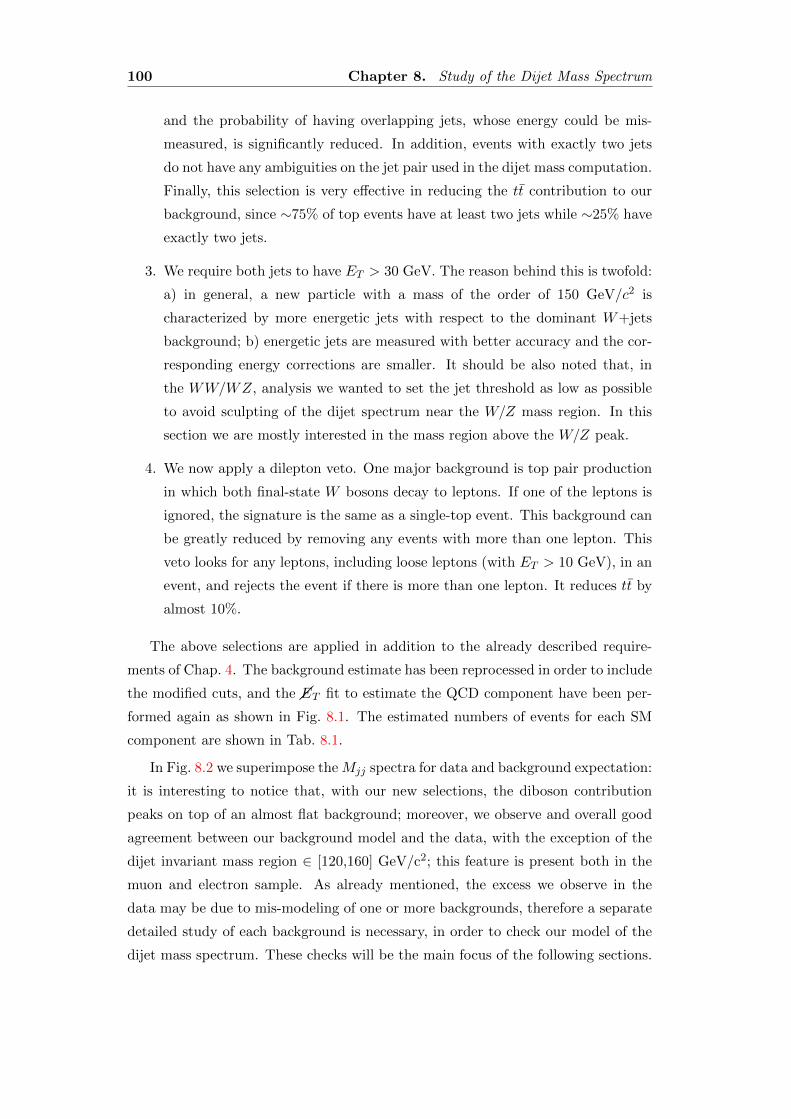
100 Chapter 8. Study of the Dijet Mass Spectrum
and the probability of having overlapping jets, whose energy could be mis-
measured, is significantly reduced. In addition, events with exactly two jets
do not have any ambiguities on the jet pair used in the dijet mass computation.
Finally, this selection is very effective in reducing the tt contribution to our
background, since ∼75% of top events have at least two jets while ∼25% have
exactly two jets.
3. We require both jets to have ET > 30 GeV. The reason behind this is twofold:
a) in general, a new particle with a mass of the order of 150 GeV/c2 is
characterized by more energetic jets with respect to the dominant W+jets
background; b) energetic jets are measured with better accuracy and the cor-
responding energy corrections are smaller. It should be also noted that, in
the WW/WZ, analysis we wanted to set the jet threshold as low as possible
to avoid sculpting of the dijet spectrum near the W/Z mass region. In this
section we are mostly interested in the mass region above the W/Z peak.
4. We now apply a dilepton veto. One major background is top pair production
in which both final-state W bosons decay to leptons. If one of the leptons is
ignored, the signature is the same as a single-top event. This background can
be greatly reduced by removing any events with more than one lepton. This
veto looks for any leptons, including loose leptons (with ET > 10 GeV), in an
event, and rejects the event if there is more than one lepton. It reduces tt by
almost 10%.
The above selections are applied in addition to the already described require-
ments of Chap. 4. The background estimate has been reprocessed in order to include
the modified cuts, and the ��ET fit to estimate the QCD component have been per-
formed again as shown in Fig. 8.1. The estimated numbers of events for each SM
component are shown in Tab. 8.1.
In Fig. 8.2 we superimpose theMjj spectra for data and background expectation:
it is interesting to notice that, with our new selections, the diboson contribution
peaks on top of an almost flat background; moreover, we observe and overall good
agreement between our background model and the data, with the exception of the
dijet invariant mass region ∈ [120,160] GeV/c2; this feature is present both in the
muon and electron sample. As already mentioned, the excess we observe in the
data may be due to mis-modeling of one or more backgrounds, therefore a separate
detailed study of each background is necessary, in order to check our model of the
dijet mass spectrum. These checks will be the main focus of the following sections.
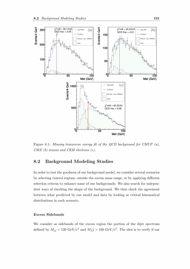
8.2 Background Modeling Studies 101
Met (GeV)0 50 100
Events
/4 G
eV
0
100
200
300 /ndf = 36.14/242χ Data CMUP
Fit Result
W/Z+jet + Top + WW/WZ
QCD
QCD frac = 2.65
Met (GeV)0 50 100
Events
/4 G
eV
0
100
200
300
1 = 4.30 fbL dt∫CDF Run II Preliminary
(a)
Met (GeV)0 50 100
Events
/4 G
eV
0
50
100
150
/ndf = 26.02/242χ Data CMX
Fit Result
W/Z+jet + Top + WW/WZ
QCD
QCD frac = 4.61
Met (GeV)0 50 100
Events
/4 G
eV
0
50
100
150
1 = 4.30 fbL dt∫CDF Run II Preliminary
(b)
Met (GeV)0 50 100
Events
/4 G
eV
0
500
1000
/ndf = 42.42/242χ
Data CEM
Fit Result
W/Z+jet + Top + WW/WZ
QCD
QCD frac = 6.98
Met (GeV)0 50 100
Events
/4 G
eV
0
500
1000
1 = 4.30 fbL dt∫CDF Run II Preliminary
(c)
Figure 8.1: Missing transverse energy fit of the QCD background for CMUP (a),
CMX (b) muons and CEM electrons (c).
8.2 Background Modeling Studies
In order to test the goodness of our background model, we consider several scenarios
by selecting control regions, outside the excess mass range, or by applying different
selection criteria to enhance some of our backgrounds. We also search for indepen-
dent ways of checking the shape of the background. We then check the agreement
between what predicted by our model and data by looking at critical kinematical
distributions in each scenario.
Excess Sidebands
We consider as sidebands of the excess region the portion of the dijet spectrum
defined by Mjj < 120 GeV/c2 and Mjj > 160 GeV/c2. The idea is to verify if our
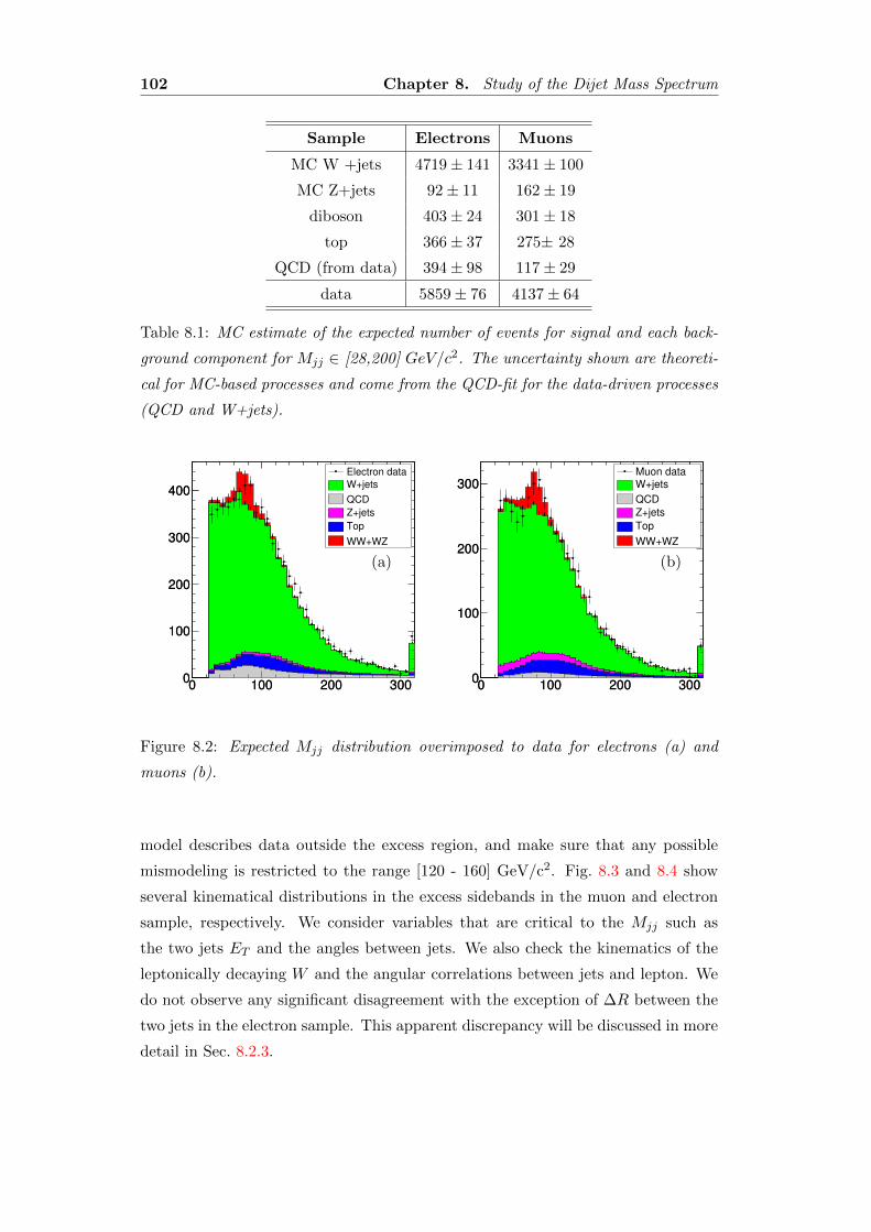
102 Chapter 8. Study of the Dijet Mass Spectrum
Sample Electrons Muons
MC W +jets 4719± 141 3341± 100
MC Z+jets 92± 11 162± 19
diboson 403± 24 301± 18
top 366± 37 275± 28
QCD (from data) 394± 98 117± 29
data 5859± 76 4137± 64
Table 8.1: MC estimate of the expected number of events for signal and each back-
ground component for Mjj ∈ [28,200] GeV/c2. The uncertainty shown are theoreti-
cal for MC-based processes and come from the QCD-fit for the data-driven processes
(QCD and W+jets).
0 100 200 3000
100
200
300
400
0 100 200 3000
100
200
300
400
Electron data
W+jets
QCD
Z+jets
Top
WW+WZ
(a)
0 100 200 3000
100
200
300
0 100 200 3000
100
200
300Muon dataW+jets
QCD
Z+jets
Top
WW+WZ
(b)
Figure 8.2: Expected Mjj distribution overimposed to data for electrons (a) and
muons (b).
model describes data outside the excess region, and make sure that any possible
mismodeling is restricted to the range [120 - 160] GeV/c2. Fig. 8.3 and 8.4 show
several kinematical distributions in the excess sidebands in the muon and electron
sample, respectively. We consider variables that are critical to the Mjj such as
the two jets ET and the angles between jets. We also check the kinematics of the
leptonically decaying W and the angular correlations between jets and lepton. We
do not observe any significant disagreement with the exception of ∆R between the
two jets in the electron sample. This apparent discrepancy will be discussed in more
detail in Sec. 8.2.3.
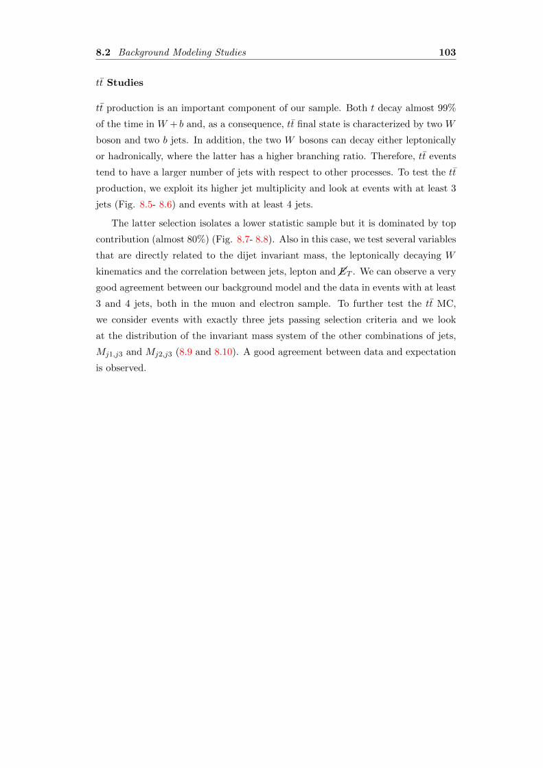
8.2 Background Modeling Studies 103
tt Studies
tt production is an important component of our sample. Both t decay almost 99%
of the time in W + b and, as a consequence, tt final state is characterized by two W
boson and two b jets. In addition, the two W bosons can decay either leptonically
or hadronically, where the latter has a higher branching ratio. Therefore, tt events
tend to have a larger number of jets with respect to other processes. To test the tt
production, we exploit its higher jet multiplicity and look at events with at least 3
jets (Fig. 8.5- 8.6) and events with at least 4 jets.
The latter selection isolates a lower statistic sample but it is dominated by top
contribution (almost 80%) (Fig. 8.7- 8.8). Also in this case, we test several variables
that are directly related to the dijet invariant mass, the leptonically decaying W
kinematics and the correlation between jets, lepton and ��ET . We can observe a very
good agreement between our background model and the data in events with at least
3 and 4 jets, both in the muon and electron sample. To further test the tt MC,
we consider events with exactly three jets passing selection criteria and we look
at the distribution of the invariant mass system of the other combinations of jets,
Mj1,j3 and Mj2,j3 (8.9 and 8.10). A good agreement between data and expectation
is observed.
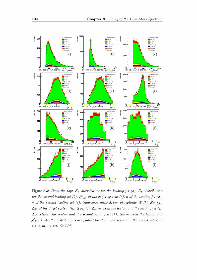
104 Chapter 8. Study of the Dijet Mass Spectrum
GeV Tjet1 E0 50 100 150 200
Entr
ies
0
100
200
300
0 50 100 150 2000
100
200
300CMUP+CMX Data
WW/WZ
W + jets
Multijet
+ jetsντ →W
ll + jets→Z
+ single ttt
uncertainty
/ndf= 38.6/ 42 2χKS = 91.3 %,
(a)
GeV Tjet2 E0 50 100 150
Entr
ies
0
500
1000
0 50 100 1500
500
1000CMUP+CMX Data
WW/WZ
W + jets
Multijet
+ jetsντ →W
ll + jets→Z
+ single ttt
uncertainty
/ndf= 82.0/ 42 2χKS = 17.8 %,
(b)
GeV/c T,j1j2
P0 50 100 150 200
Entr
ies
0
200
400
0 50 100 150 2000
200
400
CMUP+CMX Data
WW/WZ
W + jets
Multijet
+ jetsντ →W
ll + jets→Z
+ single ttt
uncertainty
/ndf= 24.5/ 19 2χKS = 88.0 %,
(c)
ηjet1 -2 0 2
Entr
ies
0
100
200
300
-2 0 20
100
200
300
CMUP+CMX Data
WW/WZ
W + jets
Multijet
+ jetsντ →W
ll + jets→Z
+ single ttt
uncertainty
/ndf= 15.1/ 23 2χKS = 16.2 %,
(d)
ηjet2 -2 0 2
Entr
ies
0
100
200
300
-2 0 20
100
200
300CMUP+CMX Data
WW/WZ
W + jets
Multijet
+ jetsντ →W
ll + jets→Z
+ single ttt
uncertainty
/ndf= 21.6/ 23 2χKS = 46.4 %,
(e)
2W GeV/cTM0 50 100 150
Entr
ies
0
100
200
300
400
0 50 100 1500
100
200
300
400 CMUP+CMX Data
WW/WZ
W + jets
Multijet
+ jetsντ →W
ll + jets→Z
+ single ttt
uncertainty
/ndf= 96.7/ 42 2χKS = 19.4 %,
(f)
MET GeV 0 50 100 150
Entr
ies
0
100
200
300
0 50 100 1500
100
200
300 CMUP+CMX Data
WW/WZ
W + jets
Multijet
+ jetsντ →W
ll + jets→Z
+ single ttt
uncertainty
/ndf= 94.6/ 43 2χKS = 21.8 %,
(g)
jj
R∆0 1 2 3 4 5
Entr
ies
0
200
400
600
800
0 1 2 3 4 50
200
400
600
800CMUP+CMX Data
WW/WZ
W + jets
Multijet
+ jetsντ →W
ll + jets→Z
+ single ttt
uncertainty
/ndf= 9.1/ 8 2χKS = 32.5 %,
(h)
jj
φ ∆0 1 2 3 4 5
Entr
ies
0
100
200
300
400
0 1 2 3 4 50
100
200
300
400 CMUP+CMX Data
WW/WZ
W + jets
Multijet
+ jetsντ →W
ll + jets→Z
+ single ttt
uncertainty
/ndf= 9.8/ 12 2χKS = 40.2 %,
(i)
lep,j1
φ ∆0 1 2 3 4 5
Entr
ies
0
100
200
300
0 1 2 3 4 50
100
200
300CMUP+CMX Data
WW/WZ
W + jets
Multijet
+ jetsντ →W
ll + jets→Z
+ single ttt
uncertainty
/ndf= 26.8/ 25 2χKS = 40.0 %,
(j)
lep,j2
φ ∆0 1 2 3 4 5
Entr
ies
0
100
200
0 1 2 3 4 50
100
200
CMUP+CMX Data
WW/WZ
W + jets
Multijet
+ jetsντ →W
ll + jets→Z
+ single ttt
uncertainty
/ndf= 32.6/ 25 2χKS = 5.6 %,
(k)
lep,met
φ ∆0 1 2 3 4 5
Entr
ies
0
50
100
150
0 1 2 3 4 50
50
100
150CMUP+CMX Data
WW/WZ
W + jets
Multijet
+ jetsντ →W
ll + jets→Z
+ single ttt
uncertainty
/ndf= 29.6/ 24 2χKS = 71.4 %,
(l)
Figure 8.3: From the top: ET distribution for the leading jet (a), ET distribution
for the second leading jet (b), PT,jj of the di-jet system (c), η of the leading jet (d),
η of the second leading jet (e), transverse mass MT,W of leptonic W (f), ��ET (g),
∆R of the di-jet system (h), ∆φjj (i), ∆φ between the lepton and the leading jet (j),
∆φ between the lepton and the second leading jet (k), ∆φ between the lepton and
��ET (l). All the distributions are plotted for the muon sample in the excess sideband
120 > mjj > 160 GeV/c2.
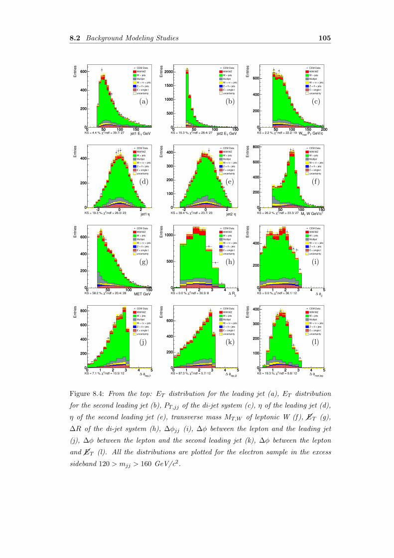
8.2 Background Modeling Studies 105
GeV Tjet1 E0 50 100 150
Entr
ies
0
200
400
600
0 50 100 1500
200
400
600
/ndf = 39.7/ 27 2χKS = 4.4 %,
CEM Data
WW/WZ
W + jets
Multijet
+ jetsντ →W
ll + jets→Z
+ single ttt
uncertainty
(a)
GeV Tjet2 E0 50 100 150
Entr
ies
0
500
1000
1500
2000
0 50 100 1500
500
1000
1500
2000
/ndf = 28.4/ 27 2χKS = 15.3 %,
CEM Data
WW/WZ
W + jets
Multijet
+ jetsντ →W
ll + jets→Z
+ single ttt
uncertainty
(b)
GeV/c T PhadW0 50 100 150 200
Entr
ies
0
200
400
600
0 50 100 150 2000
200
400
600
/ndf = 22.2/ 19 2χKS = 2.2 %,
CEM Data
WW/WZ
W + jets
Multijet
+ jetsντ →W
ll + jets→Z
+ single ttt
uncertainty
(c)
ηjet1 -2 0 2
Entr
ies
0
200
400
-2 0 20
200
400
/ndf = 26.0/ 23 2χKS = 19.3 %,
CEM Data
WW/WZ
W + jets
Multijet
+ jetsντ →W
ll + jets→Z
+ single ttt
uncertainty
(d)
ηjet2 -2 0 2
Entr
ies
0
100
200
300
400
-2 0 20
100
200
300
400
/ndf = 23.7/ 23 2χKS = 39.4 %,
CEM Data
WW/WZ
W + jets
Multijet
+ jetsντ →W
ll + jets→Z
+ single ttt
uncertainty
(e)
2 W GeV/cTM0 50 100 150
Entr
ies
0
200
400
600
800
0 50 100 1500
200
400
600
800
/ndf = 33.3/ 27 2χKS = 26.2 %,
CEM Data
WW/WZ
W + jets
Multijet
+ jetsντ →W
ll + jets→Z
+ single ttt
uncertainty
(f)
MET GeV 0 50 100 150
Entr
ies
0
200
400
600
0 50 100 1500
200
400
600
/ndf = 20.4/ 28 2χKS = 58.2 %,
CEM Data
WW/WZ
W + jets
Multijet
+ jetsντ →W
ll + jets→Z
+ single ttt
uncertainty
(g)
jj
R∆0 1 2 3 4 5
Entr
ies
0
500
1000
0 1 2 3 4 50
500
1000
/ndf = 30.3/ 8 2χKS = 0.0 %,
CEM Data
WW/WZ
W + jets
Multijet
+ jetsντ →W
ll + jets→Z
+ single ttt
uncertainty
(h)
jj
φ ∆0 1 2 3 4 5
Entr
ies
0
200
400
0 1 2 3 4 50
200
400
/ndf = 36.1/ 12 2χKS = 0.0 %,
CEM Data
WW/WZ
W + jets
Multijet
+ jetsντ →W
ll + jets→Z
+ single ttt
uncertainty
(i)
lep,j1
φ ∆0 1 2 3 4 5
Entr
ies
0
200
400
600
800
0 1 2 3 4 50
200
400
600
800
/ndf = 10.5/ 12 2χKS = 7.1 %,
CEM Data
WW/WZ
W + jets
Multijet
+ jetsντ →W
ll + jets→Z
+ single ttt
uncertainty
(j)
lep,j2
φ ∆0 1 2 3 4 5
Entr
ies
0
200
400
600
0 1 2 3 4 50
200
400
600
/ndf = 5.7/ 12 2χKS = 87.3 %,
CEM Data
WW/WZ
W + jets
Multijet
+ jetsντ →W
ll + jets→Z
+ single ttt
uncertainty
(k)
met,lep
φ ∆0 1 2 3 4 5
Entr
ies
0
100
200
300
400
0 1 2 3 4 50
100
200
300
400
/ndf = 9.8/ 12 2χKS = 19.3 %,
CEM Data
WW/WZ
W + jets
Multijet
+ jetsντ →W
ll + jets→Z
+ single ttt
uncertainty
(l)
Figure 8.4: From the top: ET distribution for the leading jet (a), ET distribution
for the second leading jet (b), PT,jj of the di-jet system (c), η of the leading jet (d),
η of the second leading jet (e), transverse mass MT,W of leptonic W (f), ��ET (g),
∆R of the di-jet system (h), ∆φjj (i), ∆φ between the lepton and the leading jet
(j), ∆φ between the lepton and the second leading jet (k), ∆φ between the lepton
and ��ET (l). All the distributions are plotted for the electron sample in the excess
sideband 120 > mjj > 160 GeV/c2.
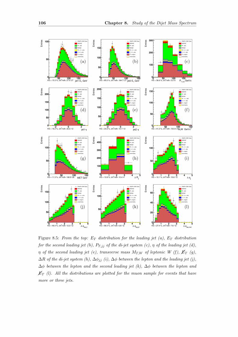
106 Chapter 8. Study of the Dijet Mass Spectrum
GeV Tjet1 E0 50 100 150
Entr
ies
0
50
100
0 50 100 1500
50
100 CMUP+CMX Data
WW/WZ
W + jets
Multijet
+ jetsντ →W
ll + jets→Z
+ single ttt
uncertainty
/ndf= 27.0/ 27 2
KS = 15.3 %, chi
(a)
GeV Tjet2 E0 50 100 150
Entr
ies
0
50
100
150
0 50 100 1500
50
100
150
CMUP+CMX Data
WW/WZ
W + jets
Multijet
+ jetsντ →W
ll + jets→Z
+ single ttt
uncertainty
/ndf= 164.7/ 27 2
KS = 85.0 %, chi
(b)
GeV/c T,j1j2
P0 50 100 150
Entr
ies
0
100
200
300
0 50 100 1500
100
200
300 CMUP+CMX Data
WW/WZ
W + jets
Multijet
+ jetsντ →W
ll + jets→Z
+ single ttt
uncertainty
/ndf= 5.2/ 6 2
KS = 36.6 %, chi
(c)
ηjet1 -2 0 2
Entr
ies
0
50
100
150
200
-2 0 20
50
100
150
200
CMUP+CMX Data
WW/WZ
W + jets
Multijet
+ jetsντ →W
ll + jets→Z
+ single ttt
uncertainty
/ndf= 26.5/ 12 2
KS = 18.2 %, chi
(d)
ηjet2 -2 0 2
Entr
ies
0
50
100
150
200
-2 0 20
50
100
150
200 CMUP+CMX Data
WW/WZ
W + jets
Multijet
+ jetsντ →W
ll + jets→Z
+ single ttt
uncertainty
/ndf= 10.7/ 12 2
KS = 24.6 %, chi
(e)
2W GeV/cTM0 50 100 150
Entr
ies
0
50
100
150
0 50 100 1500
50
100
150CMUP+CMX Data
WW/WZ
W + jets
Multijet
+ jetsντ →W
ll + jets→Z
+ single ttt
uncertainty
/ndf= 725.9/ 27 2
KS = 41.2 %, chi
(f)
MET GeV 0 50 100 150
Entr
ies
0
50
100
0 50 100 1500
50
100
CMUP+CMX Data
WW/WZ
W + jets
Multijet
+ jetsντ →W
ll + jets→Z
+ single ttt
uncertainty
/ndf= 166.9/ 28 2
KS = 11.3 %, chi
(g)
jj
R∆
0 1 2 3 4 5
Entr
ies
0
100
200
300
400
0 1 2 3 4 50
100
200
300
400
CMUP+CMX Data
WW/WZ
W + jets
Multijet
+ jetsντ →W
ll + jets→Z
+ single ttt
uncertainty
/ndf= 10.4/ 4 2
KS = 10.8 %, chi
(h)
jj
φ ∆0 1 2 3 4 5
Entr
ies
0
50
100
0 1 2 3 4 50
50
100
CMUP+CMX Data
WW/WZ
W + jets
Multijet
+ jetsντ →W
ll + jets→Z
+ single ttt
uncertainty
/ndf= 19.6/ 12 2
KS = 10.1 %, chi
(i)
lep,j1
φ ∆0 1 2 3 4 5
Entr
ies
0
50
100
150
0 1 2 3 4 50
50
100
150
CMUP+CMX Data
WW/WZ
W + jets
Multijet
+ jetsντ →W
ll + jets→Z
+ single ttt
uncertainty
/ndf= 12.3/ 12 2
KS = 46.0 %, chi
(j)
lep,j2
φ ∆0 1 2 3 4 5
Entr
ies
0
50
100
0 1 2 3 4 50
50
100
CMUP+CMX Data
WW/WZ
W + jets
Multijet
+ jetsντ →W
ll + jets→Z
+ single ttt
uncertainty
/ndf= 6.8/ 12 2
KS = 88.3 %, chi
(k)
lep,met
φ ∆0 1 2 3 4 5
Entr
ies
0
20
40
60
0 1 2 3 4 50
20
40
60
CMUP+CMX Data
WW/WZ
W + jets
Multijet
+ jetsντ →W
ll + jets→Z
+ single ttt
uncertainty
/ndf= 7.6/ 12 2
KS = 27.4 %, chi
(l)
Figure 8.5: From the top: ET distribution for the leading jet (a), ET distribution
for the second leading jet (b), PT,jj of the di-jet system (c), η of the leading jet (d),
η of the second leading jet (e), transverse mass MT,W of leptonic W (f), ��ET (g),
∆R of the di-jet system (h), ∆φjj (i), ∆φ between the lepton and the leading jet (j),
∆φ between the lepton and the second leading jet (k), ∆φ between the lepton and
��ET (l). All the distributions are plotted for the muon sample for events that have
more or three jets.
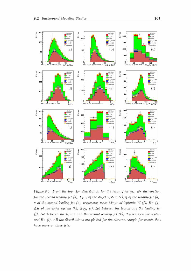
8.2 Background Modeling Studies 107
GeV Tjet1 E0 50 100 150
Entr
ies
0
50
100
150
0 50 100 1500
50
100
150
/ndf= 31.1/ 27 2χKS = 19.9 %,
CEM Data
WW/WZ
W + jets
Multijet
+ jetsντ →W
ll + jets→Z
+ single ttt
uncertainty
(a)
GeV Tjet2 E0 50 100 150
Entr
ies
0
100
200
0 50 100 1500
100
200
/ndf= 399.6/ 27 2χKS = 82.2 %,
CEM Data
WW/WZ
W + jets
Multijet
+ jetsντ →W
ll + jets→Z
+ single ttt
uncertainty
(b)
GeV/c T PhadW0 50 100 150
Entr
ies
0
100
200
300
400
0 50 100 1500
100
200
300
400
/ndf= 12.6/ 6 2χKS = 13.1 %,
CEM Data
WW/WZ
W + jets
Multijet
+ jetsντ →W
ll + jets→Z
+ single ttt
uncertainty
(c)
ηjet1 -2 0 2
Entr
ies
0
100
200
300
-2 0 20
100
200
300
/ndf= 23.7/ 12 2χKS = 7.9 %,
CEM Data
WW/WZ
W + jets
Multijet
+ jetsντ →W
ll + jets→Z
+ single ttt
uncertainty
(d)
ηjet2 -2 0 2
Entr
ies
0
100
200
-2 0 20
100
200
/ndf= 12.4/ 12 2χKS = 94.0 %,
CEM Data
WW/WZ
W + jets
Multijet
+ jetsντ →W
ll + jets→Z
+ single ttt
uncertainty
(e)
2 W GeV/cTM0 50 100 150
Entr
ies
0
50
100
150
200
0 50 100 1500
50
100
150
200
/ndf= 16.8/ 27 2χKS = 96.5 %,
CEM Data
WW/WZ
W + jets
Multijet
+ jetsντ →W
ll + jets→Z
+ single ttt
uncertainty
(f)
MET GeV 0 50 100 150
Entr
ies
0
50
100
150
200
0 50 100 1500
50
100
150
200
/ndf= 170.7/ 28 2χKS = 61.1 %,
CEM Data
WW/WZ
W + jets
Multijet
+ jetsντ →W
ll + jets→Z
+ single ttt
uncertainty
(g)
jj
R∆0 1 2 3 4 5
Entr
ies
0
200
400
600
0 1 2 3 4 50
200
400
600
/ndf= 9.1/ 4 2χKS = 28.5 %,
CEM Data
WW/WZ
W + jets
Multijet
+ jetsντ →W
ll + jets→Z
+ single ttt
uncertainty
(h)
jj
φ ∆0 1 2 3 4 5
Entr
ies
0
50
100
150
200
0 1 2 3 4 50
50
100
150
200
/ndf= 18.4/ 12 2χKS = 53.0 %,
CEM Data
WW/WZ
W + jets
Multijet
+ jetsντ →W
ll + jets→Z
+ single ttt
uncertainty
(i)
lep,j1
φ ∆0 1 2 3 4 5
Entr
ies
0
100
200
0 1 2 3 4 50
100
200
/ndf= 14.4/ 12 2χKS = 25.3 %,
CEM Data
WW/WZ
W + jets
Multijet
+ jetsντ →W
ll + jets→Z
+ single ttt
uncertainty
(j)
lep,j2
φ ∆0 1 2 3 4 5
Entr
ies
0
50
100
150
200
0 1 2 3 4 50
50
100
150
200
/ndf= 7.7/ 12 2χKS = 86.5 %,
CEM Data
WW/WZ
W + jets
Multijet
+ jetsντ →W
ll + jets→Z
+ single ttt
uncertainty
(k)
met,lep
φ ∆0 1 2 3 4 5
Entr
ies
0
50
100
0 1 2 3 4 50
50
100
/ndf= 22.2/ 12 2χKS = 41.9 %,
CEM Data
WW/WZ
W + jets
Multijet
+ jetsντ →W
ll + jets→Z
+ single ttt
uncertainty
(l)
Figure 8.6: From the top: ET distribution for the leading jet (a), ET distribution
for the second leading jet (b), PT,jj of the di-jet system (c), η of the leading jet (d),
η of the second leading jet (e), transverse mass MT,W of leptonic W (f), ��ET (g),
∆R of the di-jet system (h), ∆φjj (i), ∆φ between the lepton and the leading jet
(j), ∆φ between the lepton and the second leading jet (k), ∆φ between the lepton
and ��ET (l). All the distributions are plotted for the electron sample for events that
have more or three jets.
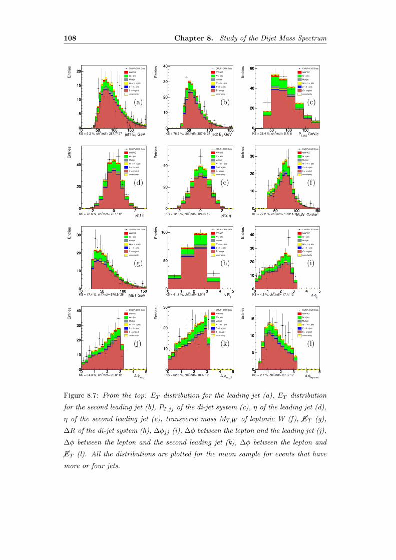
108 Chapter 8. Study of the Dijet Mass Spectrum
GeV Tjet1 E0 50 100 150
Entr
ies
0
5
10
15
20
0 50 100 1500
5
10
15
20CMUP+CMX Data
WW/WZ
W + jets
Multijet
+ jetsντ →W
ll + jets→Z
+ single ttt
uncertainty
/ndf= 287.7/ 27 2
KS = 9.2 %, chi
(a)
GeV Tjet2 E0 50 100 150
Entr
ies
0
10
20
30
40
0 50 100 1500
10
20
30
40CMUP+CMX Data
WW/WZ
W + jets
Multijet
+ jetsντ →W
ll + jets→Z
+ single ttt
uncertainty
/ndf= 357.6/ 27 2
KS = 76.5 %, chi
(b)
GeV/c T,j1j2
P0 50 100 150
Entr
ies
0
20
40
60
0 50 100 1500
20
40
60 CMUP+CMX Data
WW/WZ
W + jets
Multijet
+ jetsντ →W
ll + jets→Z
+ single ttt
uncertainty
/ndf= 5.7/ 6 2
KS = 28.4 %, chi
(c)
ηjet1 -2 0 2
Entr
ies
0
20
40
-2 0 20
20
40
CMUP+CMX Data
WW/WZ
W + jets
Multijet
+ jetsντ →W
ll + jets→Z
+ single ttt
uncertainty
/ndf= 78.1/ 12 2
KS = 78.6 %, chi
(d)
ηjet2 -2 0 2
Entr
ies
0
20
40
-2 0 20
20
40
CMUP+CMX Data
WW/WZ
W + jets
Multijet
+ jetsντ →W
ll + jets→Z
+ single ttt
uncertainty
/ndf= 124.0/ 12 2
KS = 12.5 %, chi
(e)
2W GeV/cTM0 50 100 150
Entr
ies
0
10
20
30
0 50 100 1500
10
20
30
CMUP+CMX Data
WW/WZ
W + jets
Multijet
+ jetsντ →W
ll + jets→Z
+ single ttt
uncertainty
/ndf= 1092.1/ 27 2
KS = 77.2 %, chi
(f)
MET GeV 0 50 100 150
Entr
ies
0
10
20
30
0 50 100 1500
10
20
30
CMUP+CMX Data
WW/WZ
W + jets
Multijet
+ jetsντ →W
ll + jets→Z
+ single ttt
uncertainty
/ndf= 670.9/ 28 2
KS = 17.4 %, chi
(g)
jj
R∆
0 1 2 3 4 5
Entr
ies
0
50
100
0 1 2 3 4 50
50
100CMUP+CMX Data
WW/WZ
W + jets
Multijet
+ jetsντ →W
ll + jets→Z
+ single ttt
uncertainty
/ndf= 3.5/ 4 2
KS = 41.1 %, chi
(h)
jj
φ ∆0 1 2 3 4 5
Entr
ies
0
10
20
30
40
0 1 2 3 4 50
10
20
30
40
CMUP+CMX Data
WW/WZ
W + jets
Multijet
+ jetsντ →W
ll + jets→Z
+ single ttt
uncertainty
/ndf= 17.4/ 12 2
KS = 4.2 %, chi
(i)
lep,j1
φ ∆0 1 2 3 4 5
Entr
ies
0
10
20
30
40
0 1 2 3 4 50
10
20
30
40 CMUP+CMX Data
WW/WZ
W + jets
Multijet
+ jetsντ →W
ll + jets→Z
+ single ttt
uncertainty
/ndf= 20.8/ 12 2
KS = 34.3 %, chi
(j)
lep,j2
φ ∆0 1 2 3 4 5
Entr
ies
0
10
20
30
0 1 2 3 4 50
10
20
30CMUP+CMX Data
WW/WZ
W + jets
Multijet
+ jetsντ →W
ll + jets→Z
+ single ttt
uncertainty
/ndf= 18.4/ 12 2
KS = 62.6 %, chi
(k)
lep,met
φ ∆0 1 2 3 4 5
Entr
ies
0
5
10
15
0 1 2 3 4 50
5
10
15
CMUP+CMX Data
WW/WZ
W + jets
Multijet
+ jetsντ →W
ll + jets→Z
+ single ttt
uncertainty
/ndf= 27.3/ 12 2
KS = 2.7 %, chi
(l)
Figure 8.7: From the top: ET distribution for the leading jet (a), ET distribution
for the second leading jet (b), PT,jj of the di-jet system (c), η of the leading jet (d),
η of the second leading jet (e), transverse mass MT,W of leptonic W (f), ��ET (g),
∆R of the di-jet system (h), ∆φjj (i), ∆φ between the lepton and the leading jet (j),
∆φ between the lepton and the second leading jet (k), ∆φ between the lepton and
��ET (l). All the distributions are plotted for the muon sample for events that have
more or four jets.
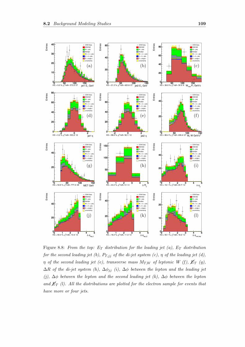
8.2 Background Modeling Studies 109
GeV Tjet1 E0 50 100 150
Entr
ies
0
10
20
30
40
0 50 100 1500
10
20
30
40
/ndf= 572.2/ 27 2χKS = 0.0 %,
CEM Data
WW/WZ
W + jets
Multijet
+ jetsντ →W
ll + jets→Z
+ single ttt
uncertainty
(a)
GeV Tjet2 E0 50 100 150
Entr
ies
0
20
40
60
0 50 100 1500
20
40
60
/ndf= 422.6/ 27 2χKS = 21.3 %,
CEM Data
WW/WZ
W + jets
Multijet
+ jetsντ →W
ll + jets→Z
+ single ttt
uncertainty
(b)
GeV/c T PhadW0 50 100 150
Entr
ies
0
20
40
60
80
0 50 100 1500
20
40
60
80
/ndf= 30.5/ 6 2χKS = 36.9 %,
CEM Data
WW/WZ
W + jets
Multijet
+ jetsντ →W
ll + jets→Z
+ single ttt
uncertainty
(c)
ηjet1 -2 0 2
Entr
ies
0
20
40
60
80
-2 0 20
20
40
60
80
/ndf= 335.2/ 12 2χKS = 0.2 %,
CEM Data
WW/WZ
W + jets
Multijet
+ jetsντ →W
ll + jets→Z
+ single ttt
uncertainty
(d)
ηjet2 -2 0 2
Entr
ies
0
20
40
60
-2 0 20
20
40
60
/ndf= 92.1/ 12 2χKS = 98.6 %,
CEM Data
WW/WZ
W + jets
Multijet
+ jetsντ →W
ll + jets→Z
+ single ttt
uncertainty
(e)
2 W GeV/cTM0 50 100 150
Entr
ies
0
20
40
0 50 100 1500
20
40
/ndf= 406.4/ 27 2χKS = 86.4 %,
CEM Data
WW/WZ
W + jets
Multijet
+ jetsντ →W
ll + jets→Z
+ single ttt
uncertainty
(f)
MET GeV 0 50 100 150
Entr
ies
0
20
40
0 50 100 1500
20
40
/ndf= 777.3/ 28 2χKS = 54.9 %,
CEM Data
WW/WZ
W + jets
Multijet
+ jetsντ →W
ll + jets→Z
+ single ttt
uncertainty
(g)
jj
R∆0 1 2 3 4 5
Entr
ies
0
50
100
150
0 1 2 3 4 50
50
100
150
/ndf= 5.1/ 4 2χKS = 44.2 %,
CEM Data
WW/WZ
W + jets
Multijet
+ jetsντ →W
ll + jets→Z
+ single ttt
uncertainty
(h)
jj
φ ∆0 1 2 3 4 5
Entr
ies
0
20
40
0 1 2 3 4 50
20
40
/ndf= 20.7/ 12 2χKS = 16.1 %,
CEM Data
WW/WZ
W + jets
Multijet
+ jetsντ →W
ll + jets→Z
+ single ttt
uncertainty
(i)
lep,j1
φ ∆0 1 2 3 4 5
Entr
ies
0
20
40
0 1 2 3 4 50
20
40
/ndf= 10.4/ 12 2χKS = 93.4 %,
CEM Data
WW/WZ
W + jets
Multijet
+ jetsντ →W
ll + jets→Z
+ single ttt
uncertainty
(j)
lep,j2
φ ∆0 1 2 3 4 5
Entr
ies
0
20
40
0 1 2 3 4 50
20
40
/ndf= 11.3/ 12 2χKS = 18.2 %,
CEM Data
WW/WZ
W + jets
Multijet
+ jetsντ →W
ll + jets→Z
+ single ttt
uncertainty
(k)
met,lep
φ ∆0 1 2 3 4 5
Entr
ies
0
10
20
0 1 2 3 4 50
10
20
/ndf= 18.2/ 12 2χKS = 50.1 %,
CEM Data
WW/WZ
W + jets
Multijet
+ jetsντ →W
ll + jets→Z
+ single ttt
uncertainty
(l)
Figure 8.8: From the top: ET distribution for the leading jet (a), ET distribution
for the second leading jet (b), PT,jj of the di-jet system (c), η of the leading jet (d),
η of the second leading jet (e), transverse mass MT,W of leptonic W (f), ��ET (g),
∆R of the di-jet system (h), ∆φjj (i), ∆φ between the lepton and the leading jet
(j), ∆φ between the lepton and the second leading jet (k), ∆φ between the lepton
and ��ET (l). All the distributions are plotted for the electron sample for events that
have more or four jets.
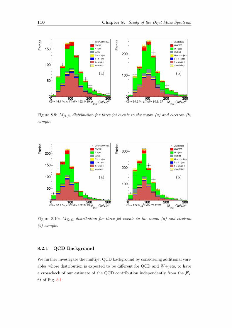
110 Chapter 8. Study of the Dijet Mass Spectrum
2 GeV/cj1,j3
M0 100 200 300
Entr
ies
0
50
100
150
0 100 200 3000
50
100
150
CMUP+CMX Data
WW/WZ
W + jets
Multijet
+ jetsντ →W
ll + jets→Z
+ single ttt
uncertainty
/ndf= 152.1/ 29 2
KS = 14.1 %, chi
(a)
2 GeV/cj1,j3
M0 100 200 300
Entr
ies
0
100
200
0 100 200 3000
100
200
/ndf= 90.8/ 27 2χKS = 24.6 %,
CEM Data
WW/WZ
W + jets
Multijet
+ jetsντ →W
ll + jets→Z
+ single ttt
uncertainty
(b)
Figure 8.9: Mj1,j3 distribution for three jet events in the muon (a) and electron (b)
sample.
2 GeV/cj2,j3
M0 100 200 300
Entr
ies
0
50
100
150
200
0 100 200 3000
50
100
150
200
CMUP+CMX Data
WW/WZ
W + jets
Multijet
+ jetsντ →W
ll + jets→Z
+ single ttt
uncertainty
/ndf= 152.2/ 23 2
KS = 10.9 %, chi
(a)
2 GeV/cj2,j3
M0 100 200 300
Entr
ies
0
100
200
300
0 100 200 3000
100
200
300
/ndf= 78.2/ 26 2χKS = 1.5 %,
CEM Data
WW/WZ
W + jets
Multijet
+ jetsντ →W
ll + jets→Z
+ single ttt
uncertainty
(b)
Figure 8.10: Mj2,j3 distribution for three jet events in the muon (a) and electron
(b) sample.
8.2.1 QCD Background
We further investigate the multijet QCD background by considering additional vari-
ables whose distribution is expected to be different for QCD and W+jets, to have
a crosscheck of our estimate of the QCD contribution independently from the ��ET
fit of Fig. 8.1.
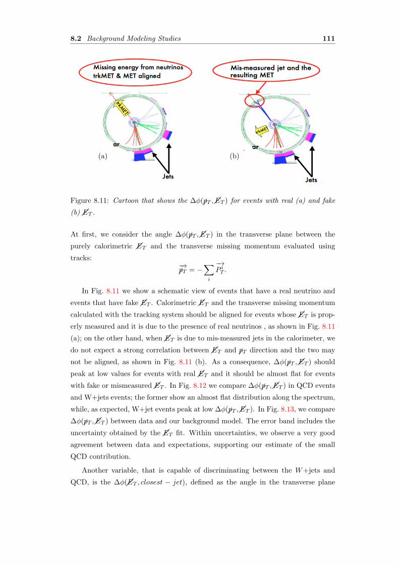
8.2 Background Modeling Studies 111
(a) (b)
Figure 8.11: Cartoon that shows the ∆φ(�pT ,��ET ) for events with real (a) and fake
(b) ��ET .
At first, we consider the angle ∆φ(�pT ,��ET ) in the transverse plane between the
purely calorimetric ��ET and the transverse missing momentum evaluated using
tracks:−→�pT = −
∑i
−→P iT .
In Fig. 8.11 we show a schematic view of events that have a real neutrino and
events that have fake ��ET . Calorimetric ��ET and the transverse missing momentum
calculated with the tracking system should be aligned for events whose ��ET is prop-
erly measured and it is due to the presence of real neutrinos , as shown in Fig. 8.11
(a); on the other hand, when ��ET is due to mis-measured jets in the calorimeter, we
do not expect a strong correlation between ��ET and �pT direction and the two may
not be aligned, as shown in Fig. 8.11 (b). As a consequence, ∆φ(�pT ,��ET ) should
peak at low values for events with real ��ET and it should be almost flat for events
with fake or mismeasured ��ET . In Fig. 8.12 we compare ∆φ(�pT ,��ET ) in QCD events
and W+jets events; the former show an almost flat distribution along the spectrum,
while, as expected, W+jet events peak at low ∆φ(�pT ,��ET ). In Fig. 8.13, we compare
∆φ(�pT ,��ET ) between data and our background model. The error band includes the
uncertainty obtained by the ��ET fit. Within uncertainties, we observe a very good
agreement between data and expectations, supporting our estimate of the small
QCD contribution.
Another variable, that is capable of discriminating between the W+jets and
QCD, is the ∆φ(��ET , closest − jet), defined as the angle in the transverse plane
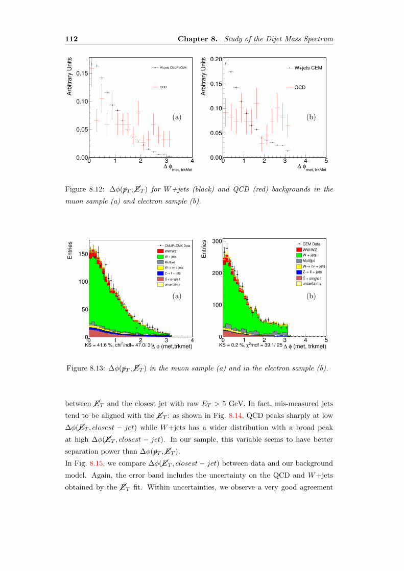
112 Chapter 8. Study of the Dijet Mass Spectrum
met, trkMetφ ∆
0 1 2 3 4
Arb
itra
ry U
nits
0.00
0.05
0.10
0.15
1 = 4.30 fbL dt∫CDF Run II Preliminary
W+jets CMUP+CMX
QCD
(a)
met, trkMetφ ∆
0 1 2 3 4 5
Arb
itra
ry U
nits
0.00
0.05
0.10
0.15
0.20
1 = 4.30 fbL dt∫CDF Run II Preliminary
W+jets CEM
QCD
(b)
Figure 8.12: ∆φ(�pT ,��ET ) for W+jets (black) and QCD (red) backgrounds in the
muon sample (a) and electron sample (b).
(met,trkmet)φ ∆0 1 2 3 4
En
trie
s
0
50
100
150
CMUP+CMX Data
WW/WZ
W + jets
Multijet
+ jetsντ →W
ll + jets→Z
+ single ttt
uncertainty
/ndf= 47.0/ 31 2
KS = 41.6 %, chi
(a)
(met, trkmet)φ ∆0 1 2 3 4 5
Entr
ies
0
100
200
300
/ndf = 39.1/ 25 2χKS = 0.2 %,
CEM Data
WW/WZ
W + jets
Multijet
+ jetsντ →W
ll + jets→Z
+ single ttt
uncertainty
(b)
Figure 8.13: ∆φ(�pT ,��ET ) in the muon sample (a) and in the electron sample (b).
between ��ET and the closest jet with raw ET > 5 GeV. In fact, mis-measured jets
tend to be aligned with the ��ET : as shown in Fig. 8.14, QCD peaks sharply at low
∆φ(��ET , closest − jet) while W+jets has a wider distribution with a broad peak
at high ∆φ(��ET , closest − jet). In our sample, this variable seems to have better
separation power than ∆φ(�pT ,��ET ).
In Fig. 8.15, we compare ∆φ(��ET , closest− jet) between data and our background
model. Again, the error band includes the uncertainty on the QCD and W+jets
obtained by the ��ET fit. Within uncertainties, we observe a very good agreement
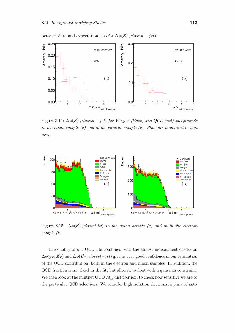
8.2 Background Modeling Studies 113
between data and expectation also for ∆φ(��ET , closest− jet).
met, closest jetφ ∆min
0 1 2 3 4 5
Arb
itra
ry U
nits
0.00
0.05
0.10
0.15
0.20
0.25
1= 4.30 fbint
CDF Run II Preliminary L
W+jets CMUP+CMX
QCD
(a)
met, closest jetφ ∆
0 1 2 3 4 5
Arb
itra
ry U
nits
0.0
0.1
0.2
0.3
1= 4.30 fbint
CDF Run II Preliminary L
W+jets CEM
QCD
(b)
Figure 8.14: ∆φ(��ET , closest− jet) for W+jets (black) and QCD (red) backgrounds
in the muon sample (a) and in the electron sample (b). Plots are nomalized to unit
area.
closest jet,met
minφ ∆0 1 2 3 4 5
Entr
ies
0
50
100
150
200CMUP+CMX Data
WW/WZ
W + jets
Multijet
+ jetsντ →W
ll + jets→Z
+ single ttt
uncertainty
/ndf= 15.4/ 24 2χKS = 84.4 %,
(a)
closest jet,met
minφ ∆0 1 2 3 4 5
Entr
ies
0
100
200
300
/ndf = 37.9/ 24 2χKS = 0.2 %,
CEM Data
WW/WZ
W + jets
Multijet
+ jetsντ →W
ll + jets→Z
+ single tttuncertainty
(b)
Figure 8.15: ∆φ(��ET , closest-jet) in the muon sample (a) and in in the electron
sample (b).
The quality of our QCD fits combined with the almost independent checks on
∆φ(�pT ,��ET ) and ∆φ(��ET , closest−jet) give us very good confidence in our estimation
of the QCD contribution, both in the electron and muon samples. In addition, the
QCD fraction is not fixed in the fit, but allowed to float with a gaussian constraint.
We then look at the multijet QCD Mjj distribution, to check how sensitive we are to
the particular QCD selections. We consider high isolation electrons in place of anti-
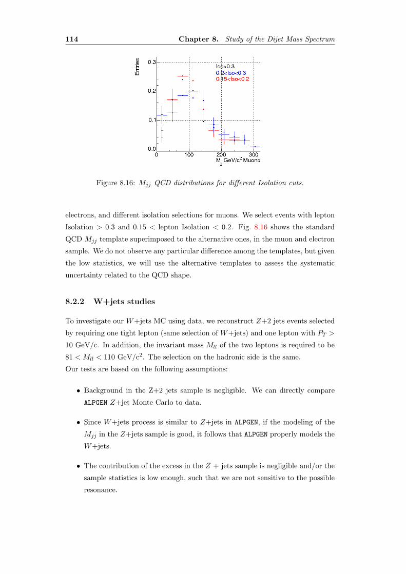
114 Chapter 8. Study of the Dijet Mass Spectrum
Figure 8.16: Mjj QCD distributions for different Isolation cuts.
electrons, and different isolation selections for muons. We select events with lepton
Isolation > 0.3 and 0.15 < lepton Isolation < 0.2. Fig. 8.16 shows the standard
QCD Mjj template superimposed to the alternative ones, in the muon and electron
sample. We do not observe any particular difference among the templates, but given
the low statistics, we will use the alternative templates to assess the systematic
uncertainty related to the QCD shape.
8.2.2 W+jets studies
To investigate our W+jets MC using data, we reconstruct Z+2 jets events selected
by requiring one tight lepton (same selection of W+jets) and one lepton with PT >
10 GeV/c. In addition, the invariant mass Mll of the two leptons is required to be
81 < Mll < 110 GeV/c2. The selection on the hadronic side is the same.
Our tests are based on the following assumptions:
• Background in the Z+2 jets sample is negligible. We can directly compare
ALPGEN Z+jet Monte Carlo to data.
• Since W+jets process is similar to Z+jets in ALPGEN, if the modeling of the
Mjj in the Z+jets sample is good, it follows that ALPGEN properly models the
W+jets.
• The contribution of the excess in the Z + jets sample is negligible and/or the
sample statistics is low enough, such that we are not sensitive to the possible
resonance.
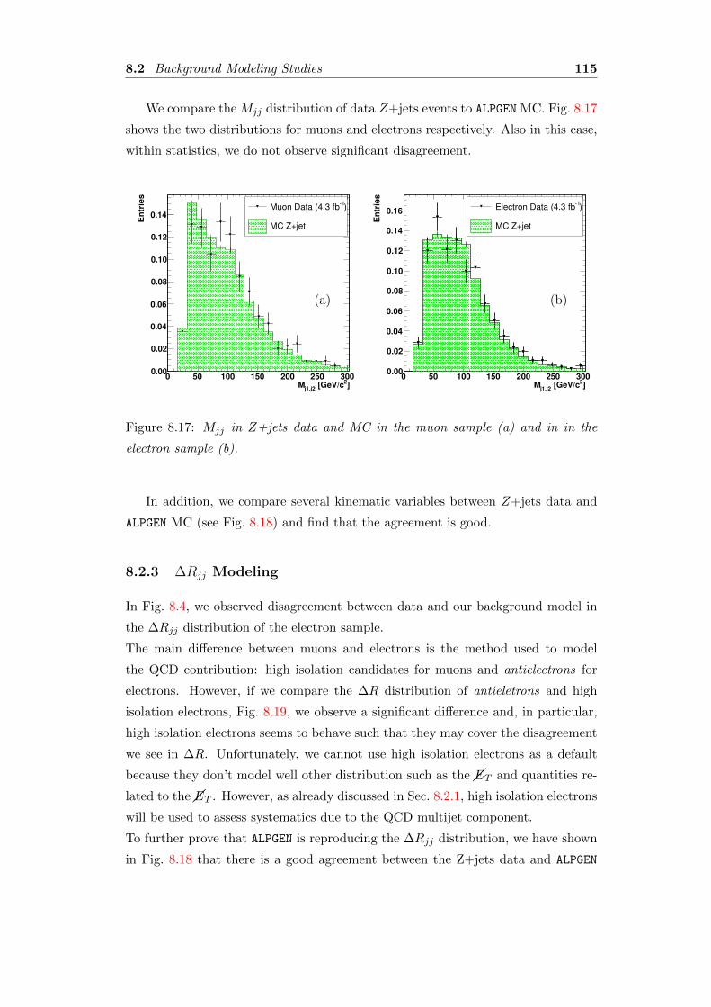
8.2 Background Modeling Studies 115
We compare the Mjj distribution of data Z+jets events to ALPGEN MC. Fig. 8.17
shows the two distributions for muons and electrons respectively. Also in this case,
within statistics, we do not observe significant disagreement.
]2 [GeV/cj1,j2
M0 50 100 150 200 250 300
En
trie
s
0.00
0.02
0.04
0.06
0.08
0.10
0.12
0.14)
1Muon Data (4.3 fb
MC Z+jet
(a)
]2 [GeV/cj1,j2
M0 50 100 150 200 250 300
En
trie
s0.00
0.02
0.04
0.06
0.08
0.10
0.12
0.14
0.16 )1
Electron Data (4.3 fb
MC Z+jet
(b)
Figure 8.17: Mjj in Z+jets data and MC in the muon sample (a) and in in the
electron sample (b).
In addition, we compare several kinematic variables between Z+jets data and
ALPGEN MC (see Fig. 8.18) and find that the agreement is good.
8.2.3 ∆Rjj Modeling
In Fig. 8.4, we observed disagreement between data and our background model in
the ∆Rjj distribution of the electron sample.
The main difference between muons and electrons is the method used to model
the QCD contribution: high isolation candidates for muons and antielectrons for
electrons. However, if we compare the ∆R distribution of antieletrons and high
isolation electrons, Fig. 8.19, we observe a significant difference and, in particular,
high isolation electrons seems to behave such that they may cover the disagreement
we see in ∆R. Unfortunately, we cannot use high isolation electrons as a default
because they don’t model well other distribution such as the ��ET and quantities re-
lated to the��ET . However, as already discussed in Sec. 8.2.1, high isolation electrons
will be used to assess systematics due to the QCD multijet component.
To further prove that ALPGEN is reproducing the ∆Rjj distribution, we have shown
in Fig. 8.18 that there is a good agreement between the Z+jets data and ALPGEN
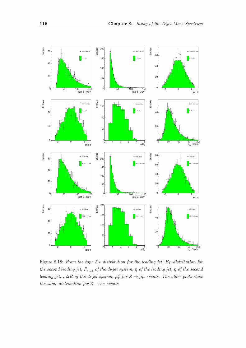
116 Chapter 8. Study of the Dijet Mass Spectrum
GeVTjet1 E0 50 100 150
Entr
ies
0
20
40
60 CMUP+CMX Data
ll + jets→Z
GeVTjet2 E0 50 100 150
Entr
ies
0
50
100
150
200CMUP+CMX Data
ll + jets→Z
ηjet1 -2 0 2
Entr
ies
0
20
40
60
CMUP+CMX Data
ll + jets→Z
ηjet2 -2 0 2
Entr
ies
0
20
40
CMUP+CMX Data
ll + jets→Z
jj R∆
0 1 2 3 4 5
En
trie
s
0
50
100
150CMUP+CMX Data
ll + jets→Z
GeV/cT,Z
p0 50 100 150 200
Entr
ies
0
20
40
CMUP+CMX Data
ll + jets→Z
GeVTjet1 E0 50 100 150
Entr
ies
0
20
40
60CEM Data
ll + jets→MC Z
GeVTjet2 E0 50 100 150
Entr
ies
0
50
100
150
200CEM Data
ll + jets→MC Z
ηjet1 -2 0 2
Entr
ies
0
20
40
60
80CEM Data
ll + jets→MC Z
ηjet2 -2 0 2
Entr
ies
0
20
40
60 CEM Data
ll + jets→MC Z
jj R∆
0 1 2 3 4 5
Entr
ies
0
50
100
150
200
CEM Data
ll + jets→MC Z
GeV/cT,Z
p0 50 100 150 200
Entr
ies
0
20
40
CEM Data
ll + jets→MC Z
Figure 8.18: From the top: ET distribution for the leading jet, ET distribution for
the second leading jet, PT,jj of the di-jet system, η of the leading jet, η of the second
leading jet, , ∆R of the di-jet system, pZT for Z → µµ events. The other plots show
the same distribution for Z → ee events.
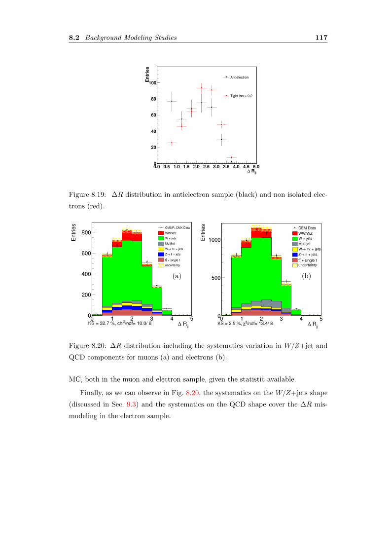
8.2 Background Modeling Studies 117
jj R∆
0.0 0.5 1.0 1.5 2.0 2.5 3.0 3.5 4.0 4.5 5.0
En
trie
s
0
20
40
60
80
100
Antielectron
Tight Iso > 0.2
Figure 8.19: ∆R distribution in antielectron sample (black) and non isolated elec-
trons (red).
jj R∆
0 1 2 3 4 5
Entr
ies
0
200
400
600
800CMUP+CMX Data
WW/WZ
W + jets
Multijet
+ jetsντ →W
ll + jets→Z
+ single ttt
uncertainty
/ndf= 10.0/ 8 2
KS = 32.7 %, chi
(a)
jj R∆0 1 2 3 4 5
En
trie
s
0
500
1000
/ndf= 13.4/ 8 2χKS = 2.5 %,
CEM Data
WW/WZ
W + jets
Multijet
+ jetsντ →W
ll + jets→Z
+ single ttt
uncertainty
(b)
Figure 8.20: ∆R distribution including the systematics variation in W/Z+jet and
QCD components for muons (a) and electrons (b).
MC, both in the muon and electron sample, given the statistic available.
Finally, as we can observe in Fig. 8.20, the systematics on the W/Z+jets shape
(discussed in Sec. 9.3) and the systematics on the QCD shape cover the ∆R mis-
modeling in the electron sample.

118 Chapter 8. Study of the Dijet Mass Spectrum
Chapter 9
Search for a Dijet Resonance
The studies performed on each of the sample component give us confidence in our
background model. While the excess we observe in the dijet invariant mass distri-
bution could still be due to a detector effect or a mis-modeling of the background
that does not show up in different kinematical regions, it is natural to ask ourselves
if the excess can be explained in terms of an additional and unexpected resonance.
9.1 Strategy
We have chosen to investigate the significance of the excess assuming an additional
gaussian component in the fit and to estimate the corresponding significance under
this assumption. The gaussian assumption is of course a simplified model, since
any dijet resonance is expected to have a slightly asymmetric distribution with a
more pronounced left tail (due to QCD radiation, out of cone jet energy and, more
in general, imprecise jet energy measurement, as we can see in the diboson MC
distribution in Figs. 6.1-6.2 (a). Moreover, the exact shape of a dijet resonance
depends on the specific physics process and the heavy flavor content of the decay
products. Given the relatively low statistics of the excess, we are not sensitive to the
details of the possible resonance shape and we prefer to use a simple gaussian model.
Since the excess in Fig. 8.2 looks narrow with respect to the detector resolution,
we search for a peak compatible with the detector resolution for a given dijet mass
value. Therefore, we can define the expected width σresonance to be equal to the
W/Z → jj width (σW/Z) scaled to the resonance mass (Mjj) in the following way:
σresonance = σW/Z
√Mjj
MW/Z(9.1)
119
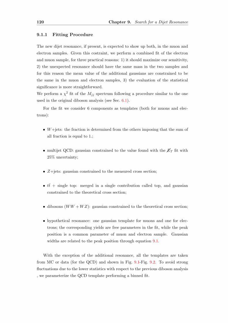
120 Chapter 9. Search for a Dijet Resonance
9.1.1 Fitting Procedure
The new dijet resonance, if present, is expected to show up both, in the muon and
electron samples. Given this costraint, we perform a combined fit of the electron
and muon sample, for three practical reasons: 1) it should maximize our sensitivity,
2) the unexpected resonance should have the same mass in the two samples and
for this reason the mean value of the additional gaussians are constrained to be
the same in the muon and electron samples, 3) the evaluation of the statistical
significance is more straightforward.
We perform a χ2 fit of the Mjj spectrum following a procedure similar to the one
used in the original diboson analysis (see Sec. 6.1).
For the fit we consider 6 components as templates (both for muons and elec-
trons):
• W+jets: the fraction is determined from the others imposing that the sum of
all fraction is equal to 1.;
• multijet QCD: gaussian constrained to the value found with the ��ET fit with
25% uncertainty;
• Z+jets: gaussian constrained to the measured cross section;
• tt + single top: merged in a single contribution called top, and gaussian
constrained to the theoretical cross section;
• dibosons (WW +WZ): gaussian constrained to the theoretical cross section;
• hypothetical resonance: one gaussian template for muons and one for elec-
trons; the corresponding yields are free parameters in the fit, while the peak
position is a common parameter of muon and electron sample. Gaussian
widths are related to the peak position through equation 9.1.
With the exception of the additional resonance, all the templates are taken
from MC or data (for the QCD) and shown in Fig. 9.1-Fig. 9.2. To avoid strong
fluctuations due to the lower statistics with respect to the previous diboson analysis
, we parameterize the QCD template performing a binned fit.
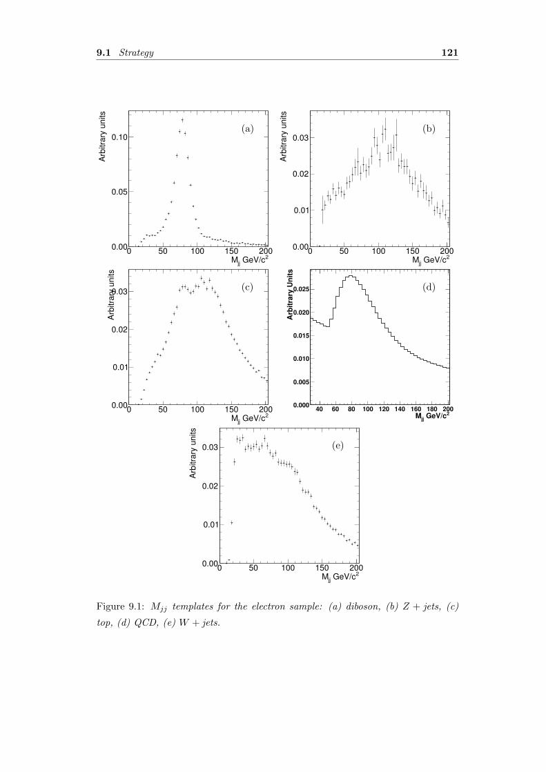
9.1 Strategy 121
2 GeV/cjjM0 50 100 150 200
Arb
itra
ry u
nits
0.00
0.05
0.10
1 = 4.30 fbL dt∫CDF Run II Preliminary
1 = 4.30 fbL dt∫CDF Run II Preliminary
(a)
2 GeV/cjjM0 50 100 150 200
Arb
itra
ry u
nits
0.00
0.01
0.02
0.03
1 = 4.30 fbL dt∫CDF Run II Preliminary
1 = 4.30 fbL dt∫CDF Run II Preliminary
(b)
2 GeV/cjjM0 50 100 150 200
Arb
itra
ry u
nits
0.00
0.01
0.02
0.03
1 = 4.30 fbL dt∫CDF Run II Preliminary
1 = 4.30 fbL dt∫CDF Run II Preliminary
(c)
2 GeV/cjj
M40 60 80 100 120 140 160 180 200
Arb
itra
ry U
nit
s
0.000
0.005
0.010
0.015
0.020
0.025
1 = 4.30 fbL dt∫CDF Run II Preliminary
(d)
2 GeV/cjjM0 50 100 150 200
Arb
itra
ry u
nits
0.00
0.01
0.02
0.03
1 = 4.30 fbL dt∫CDF Run II Preliminary
1 = 4.30 fbL dt∫CDF Run II Preliminary
(e)
Figure 9.1: Mjj templates for the electron sample: (a) diboson, (b) Z + jets, (c)
top, (d) QCD, (e) W + jets.
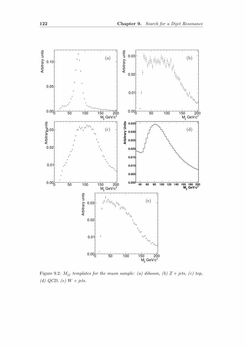
122 Chapter 9. Search for a Dijet Resonance
2 GeV/cjjM0 50 100 150 200
Arb
itra
ry u
nits
0.00
0.05
0.10
1 = 4.30 fbL dt∫CDF Run II Preliminary
1 = 4.30 fbL dt∫CDF Run II Preliminary
(a)
2 GeV/cjjM0 50 100 150 200
Arb
itra
ry u
nits
0.00
0.01
0.02
0.03
1 = 4.30 fbL dt∫CDF Run II Preliminary
1 = 4.30 fbL dt∫CDF Run II Preliminary
(b)
2 GeV/cjjM0 50 100 150 200
Arb
itra
ry u
nits
0.00
0.01
0.02
0.03
1 = 4.30 fbL dt∫CDF Run II Preliminary
1 = 4.30 fbL dt∫CDF Run II Preliminary
(c)
2 GeV/cjj
M40 60 80 100 120 140 160 180 200
Arb
itra
ry U
nit
s
0.000
0.005
0.010
0.015
0.020
0.025
0.030
0.035
1 = 4.30 fbL dt∫CDF Run II Preliminary
(d)
2 GeV/cjjM0 50 100 150 200
Arb
itra
ry u
nits
0.00
0.01
0.02
0.03
1 = 4.30 fbL dt∫CDF Run II Preliminary
1 = 4.30 fbL dt∫CDF Run II Preliminary
(e)
Figure 9.2: Mjj templates for the muon sample: (a) diboson, (b) Z + jets, (c) top,
(d) QCD, (e) W + jets.
9.2 Fit to the Data 123
9.2 Fit to the Data
Fig. 9.3 shows the projections of the fit to the data using the SM templates only.
We observe an excess at a mass of about 140 GeV/c2. The χ2 of the fit still
looks satisfactory (77.7/84), but the Kolmogorov-Smirnov (KS) test1 is poor, with
a probability of 0.0006%.
Fig. 9.4 shows the projections of the fit to the data including the additional
gaussian template. The significance is estimated using the ∆χ2 between the fit
with and without the gaussian. Since we add 3 degrees of freedom to the fit (mass,
separate yields), the ∆χ2 should have the distribution of a χ2 with 3 degrees of
freedom (this statement will be confirmed with the pseudo-experiments in Sec. 9.3).
Considering just the statistical uncertainty, we estimate a significance of 3.72σ. In
the main fit, the gaussian width is fixed to the one we expect from the experimental
resolution (14.7 GeV/c2). If we leave the width free in the fit, we estimate a width of
15.6±6.5 GeV/c2, compatible with the expectation, while the significance (without
considering systematics) is 3.6σ. It is also worth noticing that the region around
40-60 GeV, that is not well fitted in Fig. 9.3, is better described by the fit with the
addition of the gaussian component. This indicates that the SM templates alone
cannot fit the data in the region 40-60 and 130-160 GeV, unless we assume the
existence of an additional contribution. The χ2 improves by 21 and the KS tests
improves with a probability of 0.05.
In Tab. 9.1 we show the fit results, including the gaussian component for the
excess; it is also interesting to notice that the ratios between the number of events
assigned to the gaussian component and the number of expected diboson events, in
the electron and muon samples, are statistically compatible. The fit estimates the
mean of the gaussian to be 144 ± 5 GeV/c2.
The range of the fit was chosen starting from the diboson one. We also tried to
look at what happens extending the range of our fit (see Fig. 9.5). The gaussian
template describes the excess observed between 120-160 GeV/c2, while there is still
a region around 200 Gev/c2 where the background model seems to underestimate
data (the residuals show that the data points are all above the expectations) and
there seems to be a shift in the diboson template that cannot be related to the JES
(since it is measured to be 1). However, as shown in Fig. 9.5, the residuals tail
1The reported KS probability corresponds to the KS test between the data histogram and the
total MC histogram. It does not account for the fact the the MC histogram is fitted to the data.
The reported value is thus an upper limit on KS probability.
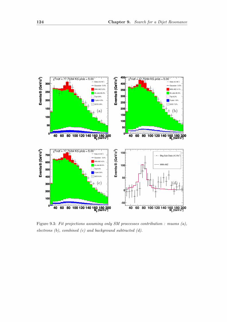
124 Chapter 9. Search for a Dijet Resonance
]2 [GeV/cjj
M40 60 80 100 120 140 160 180 200
)2
Even
ts/8
(G
eV
/c
0
50
100
150
200
250
300
/ndf = 77.73/84 KS prob = 0.002χ
]2 [GeV/cjj
M40 60 80 100 120 140 160 180 200
)2
Even
ts/8
(G
eV
/c
0
50
100
150
200
250
300)1Data (4.3 fb
Gaussian 0.0%
WW+WZ 5.0%
W+Jets 80.2%
Top 6.9%
Z+jets 4.5%
QCD 2.6%
(a)
]2 [GeV/cjj
M40 60 80 100 120 140 160 180 200
)2
Even
ts/8
(G
eV
/c
0
50
100
150
200
250
300
350
400
450/ndf = 77.73/84 KS prob = 0.002χ
]2 [GeV/cjj
M40 60 80 100 120 140 160 180 200
)2
Even
ts/8
(G
eV
/c
0
50
100
150
200
250
300
350
400
450
)1Data (4.3 fb
Gaussian 0.0%
WW+WZ 4.1%
W+Jets 80.3%
Top 6.2%
Z+jets 1.6%
QCD 7.2%
(b)
]2 [GeV/cjj
M40 60 80 100 120 140 160 180 200
)2
Even
ts/8
(G
eV
/c
0
100
200
300
400
500
600
700
/ndf = 77.73/84 KS prob = 0.002χ
]2 [GeV/cjj
M40 60 80 100 120 140 160 180 200
)2
Even
ts/8
(G
eV
/c
0
100
200
300
400
500
600
700)
1Data (4.3 fb
Gaussian 0.0%
WW+WZ 4.5%
W+Jets 80.2%
Top 6.5%
Z+jets 2.8%
QCD 5.3%
(c)
]2 [GeV/cjj
M40 60 80 100 120 140 160 180 200
)2
Even
ts/8
(G
eV
/c
50
0
50
100
150) 1Bkg Sub Data (4.3 fb
WW+WZ
) 1Bkg Sub Data (4.3 fb
WW+WZ
(d)
Figure 9.3: Fit projections assuming only SM proccesses contribution : muons (a),
electrons (b), combined (c) and background subtracted (d).
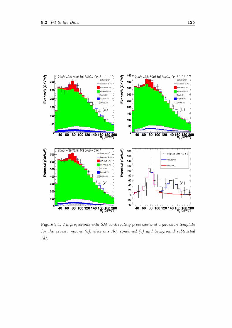
9.2 Fit to the Data 125
]2 [GeV/cjj
M40 60 80 100 120 140 160 180 200
)2
Even
ts/8
(G
eV
/c
0
50
100
150
200
250
300
/ndf = 56.73/81 KS prob = 0.222χ
]2 [GeV/cjj
M40 60 80 100 120 140 160 180 200
)2
Even
ts/8
(G
eV
/c
0
50
100
150
200
250
300)1Data (4.3 fb
Gaussian 2.4%
WW+WZ 5.2%
W+Jets 78.4%
Top 6.5%
Z+jets 4.3%
QCD 2.5%
(a)
]2 [GeV/cjj
M40 60 80 100 120 140 160 180 200
)2
Even
ts/8
(G
eV
/c
0
50
100
150
200
250
300
350
400
450/ndf = 56.73/81 KS prob = 0.232χ
]2 [GeV/cjj
M40 60 80 100 120 140 160 180 200
)2
Even
ts/8
(G
eV
/c
0
50
100
150
200
250
300
350
400
450
)1Data (4.3 fb
Gaussian 2.7%
WW+WZ 4.4%
W+Jets 78.4%
Top 5.8%
Z+jets 1.6%
QCD 6.6%
(b)
]2 [GeV/cjj
M40 60 80 100 120 140 160 180 200
)2
Even
ts/8
(G
eV
/c
0
100
200
300
400
500
600
700
/ndf = 56.73/81 KS prob = 0.042χ
]2 [GeV/cjj
M40 60 80 100 120 140 160 180 200
)2
Even
ts/8
(G
eV
/c
0
100
200
300
400
500
600
700)1Data (4.3 fb
Gaussian 2.6%
WW+WZ 4.7%
W+Jets 78.4%
Top 6.1%
Z+jets 2.7%
QCD 4.9%
(c)
]2 [GeV/cjj
M40 60 80 100 120 140 160 180 200
)2
Even
ts/8
(G
eV
/c
40
20
0
20
40
60
80
100
120
140
160
180) 1Bkg Sub Data (4.3 fb
Gaussian
WW+WZ
) 1Bkg Sub Data (4.3 fb
Gaussian
WW+WZ
(d)
Figure 9.4: Fit projections with SM contributing processes and a gaussian template
for the excess: muons (a), electrons (b), combined (c) and background subtracted
(d).

126 Chapter 9. Search for a Dijet Resonance
Parameter Electrons Muons
Excess events 156± 42 97± 38
Excess events / exp. WW+WZ 0.60± 0.18 0.44± 0.18
Gaussian mean 144± 5 GeV/c2
Table 9.1: Number of the excess events and Gaussian mean of the excess as deter-
mined by the fit. Note that the ratios of the number of events in the excess to the
number of expected diboson events in the electron and muon samples are statistically
compatible.
]2 [GeV/cjj
M50 100 150 200 250 300
)2
Even
ts/8
(G
eV
/c
0
100
200
300
400
500
600
700
]2 [GeV/cjj
M50 100 150 200 250 300
)2
Even
ts/8
(G
eV
/c
0
100
200
300
400
500
600
700)1Data (4.3 fb
Gaussian 2.3%
WW+WZ 4.5%
W+Jets 77.8%
Top 6.3%
Z+jets 2.7%
QCD 5.5%
(a)
]2 [GeV/cjjM100 200
)2E
vent
s/(8
GeV
/c
-40-20
020406080
100120140
160180
) -1Bkg Sub Data (4.3 fb
Gaussian
WW+WZ (all bkg syst.)
) -1Bkg Sub Data (4.3 fb
Gaussian
WW+WZ (all bkg syst.)
(d)
(b)
Figure 9.5: Fit projections with SM backgrounds and a gaussian template for the
excess up to 300 GeV/c2, combined (a) and background subtracted (b). The red
band represent the systematic uncertainty
around 200 GeV/c2 are within uncertainties.
9.3 Systematic and Significance
We assess the systematic uncertainty on the signal extraction considering different
sources. Those systematics will affect the number of events we estimate in our data
sample and the corresponding significance.
On the other hand, since we do not focus on any specific model for the additional
resonance search, we cannot estimate the acceptance of the gaussian and quote the
corresponding cross section. As a consequence, we will consider only the systemat-
ics affecting the signal extraction.
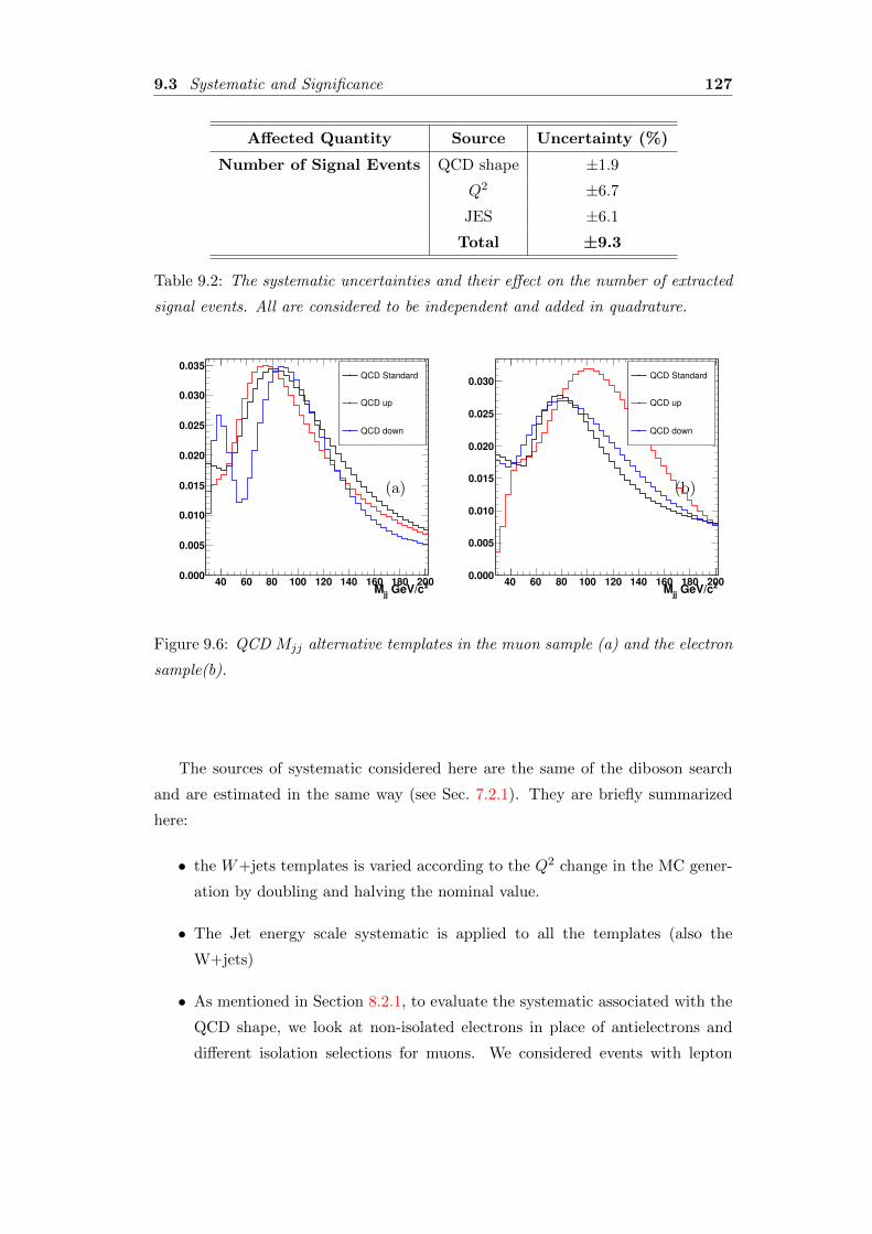
9.3 Systematic and Significance 127
Affected Quantity Source Uncertainty (%)
Number of Signal Events QCD shape ±1.9
Q2 ±6.7
JES ±6.1
Total ±9.3
Table 9.2: The systematic uncertainties and their effect on the number of extracted
signal events. All are considered to be independent and added in quadrature.
2 GeV/cjj
M40 60 80 100 120 140 160 180 200
0.000
0.005
0.010
0.015
0.020
0.025
0.030
0.035
1 = 4.30 fbL dt∫CDF Run II Preliminary
QCD Standard
QCD up
QCD down
QCD Standard
QCD up
QCD down
1 = 4.30 fbL dt∫CDF Run II Preliminary
(a)
2 GeV/cjj
M40 60 80 100 120 140 160 180 200
0.000
0.005
0.010
0.015
0.020
0.025
0.030QCD Standard
QCD up
QCD down
QCD Standard
QCD up
QCD down
(b)
Figure 9.6: QCD Mjj alternative templates in the muon sample (a) and the electron
sample(b).
The sources of systematic considered here are the same of the diboson search
and are estimated in the same way (see Sec. 7.2.1). They are briefly summarized
here:
• the W+jets templates is varied according to the Q2 change in the MC gener-
ation by doubling and halving the nominal value.
• The Jet energy scale systematic is applied to all the templates (also the
W+jets)
• As mentioned in Section 8.2.1, to evaluate the systematic associated with the
QCD shape, we look at non-isolated electrons in place of antielectrons and
different isolation selections for muons. We considered events with lepton
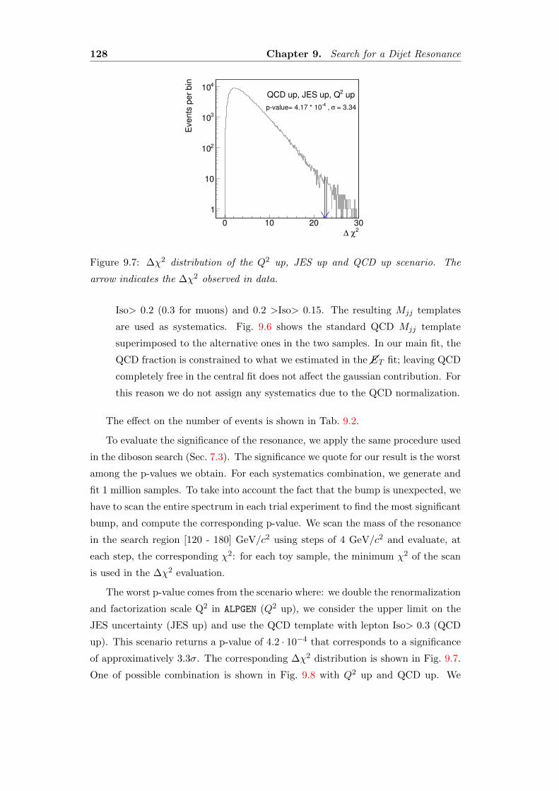
128 Chapter 9. Search for a Dijet Resonance
2χ ∆0 10 20 30
Events
per
bin
1
10
210
310
410
= 3.34σ , 4
pvalue= 4.17 * 10
1 = 4.30 fbL dt∫CDF Run II Preliminary
up2QCD up, JES up, Q
Figure 9.7: ∆χ2 distribution of the Q2 up, JES up and QCD up scenario. The
arrow indicates the ∆χ2 observed in data.
Iso> 0.2 (0.3 for muons) and 0.2 >Iso> 0.15. The resulting Mjj templates
are used as systematics. Fig. 9.6 shows the standard QCD Mjj template
superimposed to the alternative ones in the two samples. In our main fit, the
QCD fraction is constrained to what we estimated in the ��ET fit; leaving QCD
completely free in the central fit does not affect the gaussian contribution. For
this reason we do not assign any systematics due to the QCD normalization.
The effect on the number of events is shown in Tab. 9.2.
To evaluate the significance of the resonance, we apply the same procedure used
in the diboson search (Sec. 7.3). The significance we quote for our result is the worst
among the p-values we obtain. For each systematics combination, we generate and
fit 1 million samples. To take into account the fact that the bump is unexpected, we
have to scan the entire spectrum in each trial experiment to find the most significant
bump, and compute the corresponding p-value. We scan the mass of the resonance
in the search region [120 - 180] GeV/c2 using steps of 4 GeV/c2 and evaluate, at
each step, the corresponding χ2: for each toy sample, the minimum χ2 of the scan
is used in the ∆χ2 evaluation.
The worst p-value comes from the scenario where: we double the renormalization
and factorization scale Q2 in ALPGEN (Q2 up), we consider the upper limit on the
JES uncertainty (JES up) and use the QCD template with lepton Iso> 0.3 (QCD
up). This scenario returns a p-value of 4.2 · 10−4 that corresponds to a significance
of approximatively 3.3σ. The corresponding ∆χ2 distribution is shown in Fig. 9.7.
One of possible combination is shown in Fig. 9.8 with Q2 up and QCD up. We
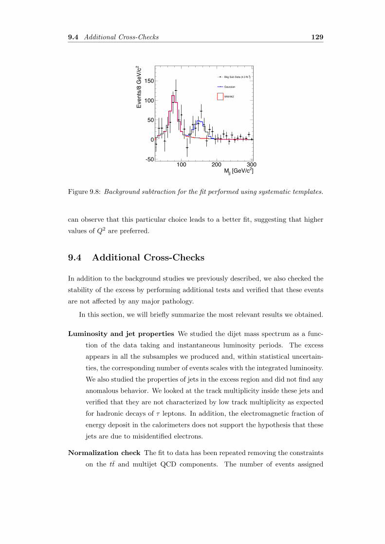
9.4 Additional Cross-Checks 129
]2 [GeV/cjjM100 200 300
2Ev
ents
/8 G
eV/c
-50
0
50
100
150)-1Bkg Sub Data (4.3 fb
Gaussian
WW/WZ
)-1Bkg Sub Data (4.3 fb
Gaussian
WW/WZ
Figure 9.8: Background subtraction for the fit performed using systematic templates.
can observe that this particular choice leads to a better fit, suggesting that higher
values of Q2 are preferred.
9.4 Additional Cross-Checks
In addition to the background studies we previously described, we also checked the
stability of the excess by performing additional tests and verified that these events
are not affected by any major pathology.
In this section, we will briefly summarize the most relevant results we obtained.
Luminosity and jet properties We studied the dijet mass spectrum as a func-
tion of the data taking and instantaneous luminosity periods. The excess
appears in all the subsamples we produced and, within statistical uncertain-
ties, the corresponding number of events scales with the integrated luminosity.
We also studied the properties of jets in the excess region and did not find any
anomalous behavior. We looked at the track multiplicity inside these jets and
verified that they are not characterized by low track multiplicity as expected
for hadronic decays of τ leptons. In addition, the electromagnetic fraction of
energy deposit in the calorimeters does not support the hypothesis that these
jets are due to misidentified electrons.
Normalization check The fit to data has been repeated removing the constraints
on the tt and multijet QCD components. The number of events assigned
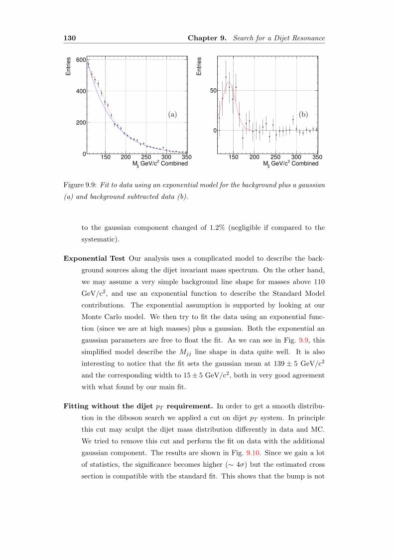
130 Chapter 9. Search for a Dijet Resonance
Combined2 GeV/cjjM150 200 250 300 350
Entr
ies
0
200
400
600
1= 4.30 fbint
CDF Run II Preliminary L 1= 4.30 fbint
CDF Run II Preliminary L
(a)
Combined2 GeV/cjjM150 200 250 300 350
Entr
ies
0
50
1= 4.30 fbint
CDF Run II Preliminary L 1= 4.30 fbint
CDF Run II Preliminary L
(b)
Figure 9.9: Fit to data using an exponential model for the background plus a gaussian
(a) and background subtracted data (b).
to the gaussian component changed of 1.2% (negligible if compared to the
systematic).
Exponential Test Our analysis uses a complicated model to describe the back-
ground sources along the dijet invariant mass spectrum. On the other hand,
we may assume a very simple background line shape for masses above 110
GeV/c2, and use an exponential function to describe the Standard Model
contributions. The exponential assumption is supported by looking at our
Monte Carlo model. We then try to fit the data using an exponential func-
tion (since we are at high masses) plus a gaussian. Both the exponential an
gaussian parameters are free to float the fit. As we can see in Fig. 9.9, this
simplified model describe the Mjj line shape in data quite well. It is also
interesting to notice that the fit sets the gaussian mean at 139 ± 5 GeV/c2
and the corresponding width to 15± 5 GeV/c2, both in very good agreement
with what found by our main fit.
Fitting without the dijet pT requirement. In order to get a smooth distribu-
tion in the diboson search we applied a cut on dijet pT system. In principle
this cut may sculpt the dijet mass distribution differently in data and MC.
We tried to remove this cut and perform the fit on data with the additional
gaussian component. The results are shown in Fig. 9.10. Since we gain a lot
of statistics, the significance becomes higher (∼ 4σ) but the estimated cross
section is compatible with the standard fit. This shows that the bump is not
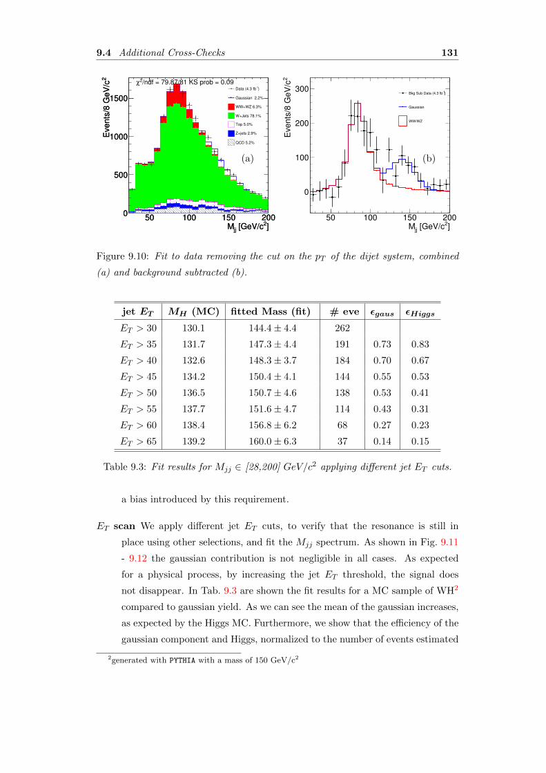
9.4 Additional Cross-Checks 131
]2 [GeV/cjjM50 100 150 200
2E
vents
/8 G
eV
/c
0
500
1000
1500
1 = 4.30 fbL dt∫CDF Run II Preliminary
/ndf = 79.87/81 KS prob = 0.092χ
]2 [GeV/cjjM50 100 150 200
2E
vents
/8 G
eV
/c
0
500
1000
1500
)1Data (4.3 fb
Gaussian 2.2%
WW+WZ 6.3%
W+Jets 78.1%
Top 5.0%
Z+jets 2.9%
QCD 5.2%
1 = 4.30 fbL dt∫CDF Run II Preliminary
(a)
]2 [GeV/cjjM50 100 150 200
2E
vents
/8 G
eV
/c
0
100
200
300
1 = 4.30 fbL dt∫CDF Run II Preliminary
)1
Bkg Sub Data (4.3 fb
Gaussian
WW/WZ
)1
Bkg Sub Data (4.3 fb
Gaussian
WW/WZ
1 = 4.30 fbL dt∫CDF Run II Preliminary
(b)
Figure 9.10: Fit to data removing the cut on the pT of the dijet system, combined
(a) and background subtracted (b).
jet ET MH (MC) fitted Mass (fit) # eve εgaus εHiggs
ET > 30 130.1 144.4± 4.4 262
ET > 35 131.7 147.3± 4.4 191 0.73 0.83
ET > 40 132.6 148.3± 3.7 184 0.70 0.67
ET > 45 134.2 150.4± 4.1 144 0.55 0.53
ET > 50 136.5 150.7± 4.6 138 0.53 0.41
ET > 55 137.7 151.6± 4.7 114 0.43 0.31
ET > 60 138.4 156.8± 6.2 68 0.27 0.23
ET > 65 139.2 160.0± 6.3 37 0.14 0.15
Table 9.3: Fit results for Mjj ∈ [28,200] GeV/c2 applying different jet ET cuts.
a bias introduced by this requirement.
ET scan We apply different jet ET cuts, to verify that the resonance is still in
place using other selections, and fit the Mjj spectrum. As shown in Fig. 9.11
- 9.12 the gaussian contribution is not negligible in all cases. As expected
for a physical process, by increasing the jet ET threshold, the signal does
not disappear. In Tab. 9.3 are shown the fit results for a MC sample of WH2
compared to gaussian yield. As we can see the mean of the gaussian increases,
as expected by the Higgs MC. Furthermore, we show that the efficiency of the
gaussian component and Higgs, normalized to the number of events estimated
2generated with PYTHIA with a mass of 150 GeV/c2
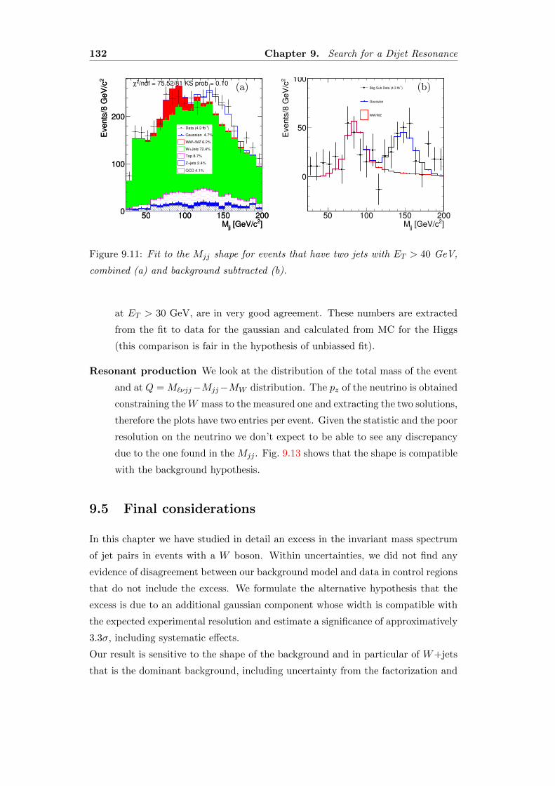
132 Chapter 9. Search for a Dijet Resonance
]2 [GeV/cjjM50 100 150 200
2E
ve
nts
/8 G
eV
/c
0
100
200
/ndf = 75.52/81 KS prob = 0.102χ
]2 [GeV/cjjM50 100 150 200
2E
ve
nts
/8 G
eV
/c
0
100
200
)1Data (4.3 fb
Gaussian 4.7%
WW+WZ 6.2%
W+Jets 72.4%
Top 8.7%
Z+jets 2.4%
QCD 4.1%
1 = 4.30 fbL dt∫CDF Run II Preliminary
(a)
]2 [GeV/cjjM50 100 150 200
2E
ve
nts
/8 G
eV
/c
0
50
100)
1Bkg Sub Data (4.3 fb
Gaussian
WW/WZ
)1
Bkg Sub Data (4.3 fb
Gaussian
WW/WZ
1 = 4.30 fbL dt∫CDF Run II Preliminary
(b)
Figure 9.11: Fit to the Mjj shape for events that have two jets with ET > 40 GeV,
combined (a) and background subtracted (b).
at ET > 30 GeV, are in very good agreement. These numbers are extracted
from the fit to data for the gaussian and calculated from MC for the Higgs
(this comparison is fair in the hypothesis of unbiassed fit).
Resonant production We look at the distribution of the total mass of the event
and at Q = M`νjj−Mjj−MW distribution. The pz of the neutrino is obtained
constraining theW mass to the measured one and extracting the two solutions,
therefore the plots have two entries per event. Given the statistic and the poor
resolution on the neutrino we don’t expect to be able to see any discrepancy
due to the one found in the Mjj . Fig. 9.13 shows that the shape is compatible
with the background hypothesis.
9.5 Final considerations
In this chapter we have studied in detail an excess in the invariant mass spectrum
of jet pairs in events with a W boson. Within uncertainties, we did not find any
evidence of disagreement between our background model and data in control regions
that do not include the excess. We formulate the alternative hypothesis that the
excess is due to an additional gaussian component whose width is compatible with
the expected experimental resolution and estimate a significance of approximatively
3.3σ, including systematic effects.
Our result is sensitive to the shape of the background and in particular of W+jets
that is the dominant background, including uncertainty from the factorization and
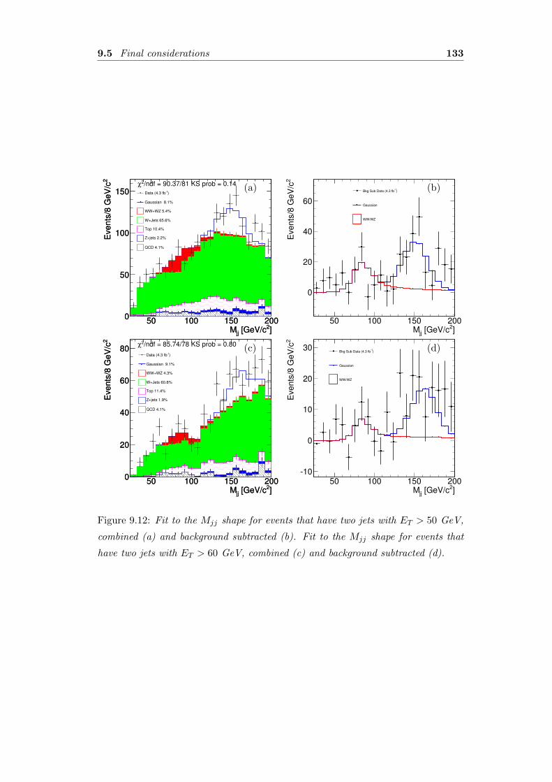
9.5 Final considerations 133
]2 [GeV/cjjM50 100 150 200
2E
vents
/8 G
eV
/c
0
50
100
150/ndf = 90.37/81 KS prob = 0.142χ
]2 [GeV/cjjM50 100 150 200
2E
vents
/8 G
eV
/c
0
50
100
150 )1Data (4.3 fb
Gaussian 8.1%
WW+WZ 5.4%
W+Jets 65.6%
Top 10.4%
Z+jets 2.2%
QCD 4.1%
1 = 4.30 fbL dt∫CDF Run II Preliminary
(a)
]2 [GeV/cjjM50 100 150 200
2E
vents
/8 G
eV
/c0
20
40
60
)1
Bkg Sub Data (4.3 fb
Gaussian
WW/WZ
)1
Bkg Sub Data (4.3 fb
Gaussian
WW/WZ
1 = 4.30 fbL dt∫CDF Run II Preliminary
(b)
]2 [GeV/cjjM50 100 150 200
2E
vents
/8 G
eV
/c
0
20
40
60
80/ndf = 85.74/78 KS prob = 0.802χ
]2 [GeV/cjjM50 100 150 200
2E
vents
/8 G
eV
/c
0
20
40
60
80)1Data (4.3 fb
Gaussian 9.1%
WW+WZ 4.3%
W+Jets 60.8%
Top 11.4%
Z+jets 1.9%
QCD 4.1%
1 = 4.30 fbL dt∫CDF Run II Preliminary
(c)
]2 [GeV/cjjM50 100 150 200
2E
vents
/8 G
eV
/c
10
0
10
20
30)
1Bkg Sub Data (4.3 fb
Gaussian
WW/WZ
)1
Bkg Sub Data (4.3 fb
Gaussian
WW/WZ
1 = 4.30 fbL dt∫CDF Run II Preliminary
(d)
Figure 9.12: Fit to the Mjj shape for events that have two jets with ET > 50 GeV,
combined (a) and background subtracted (b). Fit to the Mjj shape for events that
have two jets with ET > 60 GeV, combined (c) and background subtracted (d).
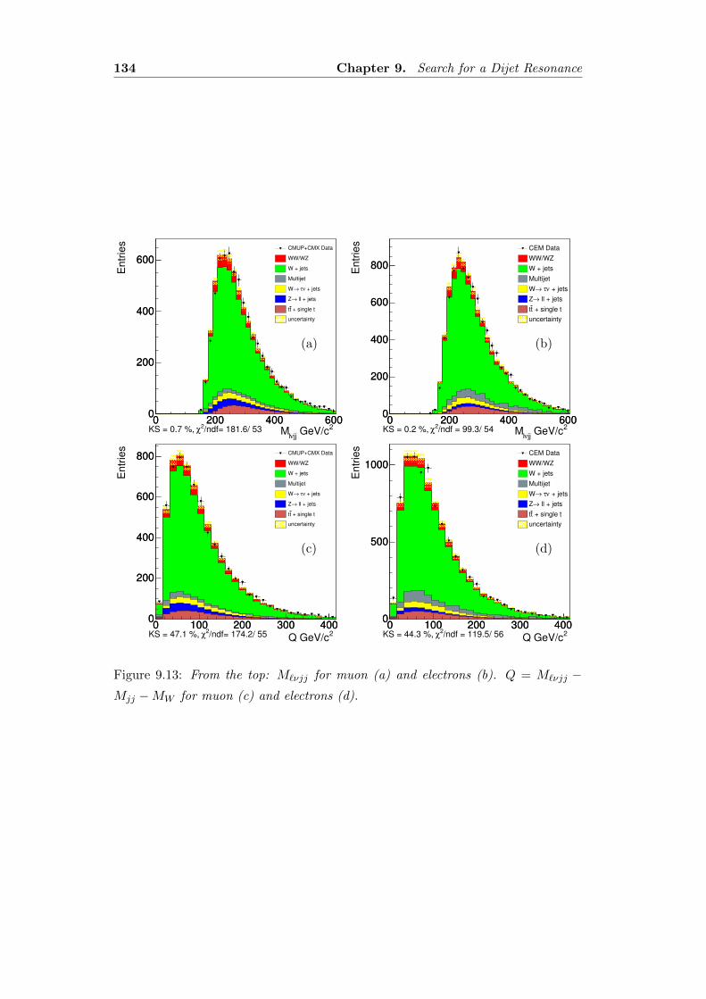
134 Chapter 9. Search for a Dijet Resonance
2 GeV/cjjνl
M0 200 400 600
Entr
ies
0
200
400
600
0 200 400 6000
200
400
600
CMUP+CMX Data
WW/WZ
W + jets
Multijet
+ jetsντ →W
ll + jets→Z
+ single ttt
uncertainty
/ndf= 181.6/ 53 2χKS = 0.7 %,
(a)
2 GeV/cjjνl
M0 200 400 600
Entr
ies
0
200
400
600
800
0 200 400 6000
200
400
600
800
/ndf = 99.3/ 54 2χKS = 0.2 %,
CEM Data
WW/WZ
W + jets
Multijet
+ jetsντ →W
ll + jets→Z
+ single ttt
uncertainty
(b)
2
Q GeV/c0 100 200 300 400
Entr
ies
0
200
400
600
800
0 100 200 300 4000
200
400
600
800 CMUP+CMX Data
WW/WZ
W + jets
Multijet
+ jetsντ →W
ll + jets→Z
+ single ttt
uncertainty
/ndf= 174.2/ 55 2χKS = 47.1 %,
(c)
2
Q GeV/c0 100 200 300 400
Entr
ies
0
500
1000
0 100 200 300 4000
500
1000
/ndf = 119.5/ 56 2χKS = 44.3 %,
CEM Data
WW/WZ
W + jets
Multijet
+ jetsντ →W
ll + jets→Z
+ single ttt
uncertainty
(d)
Figure 9.13: From the top: M`νjj for muon (a) and electrons (b). Q = M`νjj −Mjj −MW for muon (c) and electrons (d).

9.5 Final considerations 135
renormalization scales. We account for shape uncertainties in our systematics: for
W+jets we double/halve the Q2. We consider the effect of the uncertainty on our
knowledge of the jets energy scale and on the multijet model. However background
shape uncertainties (especially for W+jets) larger than the ones considered may
reduce the significance below 3σ.

136 Chapter 9. Search for a Dijet Resonance
Conclusions and Perspectives
In this thesis we presented the measurement of the WW/WZ production cross sec-
tion using the lepton plus jets final state in pp collisions at√s = 1.96 TeV. This
signature is of great interest because of its connection with the EW symmetry break-
ing of the standard model and because it allows the study of important backgrounds
for the SM Higgs boson searches, in both, low and high mass region.
This analysis used the dijet invariant mass distribution of the two leading jets in
the event to perform a fit to the data and extract the diboson content. We observe
WW/WZ events with a significance of 5.24σ and the corresponding cross section is
estimated to be :
σWW/WZ = 18.1± 3.3(stat.)± 2.5(syst.) pb,
consistent with the theoretical prediction at next-to-leading order.
The work described in this thesis, along with [24], established the capability
of CDF to extract dijet invariant mass peaks of heavy bosons over a large dijet
background. Thanks to this work, the W/Z dijet peak in the diboson sample can
be considered as a new reference to study and improve techniques to disentangle
dijet resonances over huge backgrounds: this will be crucial for low mass Higgs
searches at CDF in the W +H → lνbb. Moreover, any dijet resonance search may
benefit from the work described in this thesis and its results.
Currently, the WW +WZ cross section measurement is dominated by the sta-
tistical uncertainty and exploiting the whole integrated luminosity delivered at the
Tevatron by the end of RUN II will certainly result in a more precise cross section
measurement. In particular, by the end of 2011, CDF should have about 10 fb−1,
more than double of the luminosity used in this thesis. Additional data will be
fundamental also to convert this measurement into a TGC measurement to probe
the abelian structure of the SM, either to find deviations or to set more stringent
limits.
137
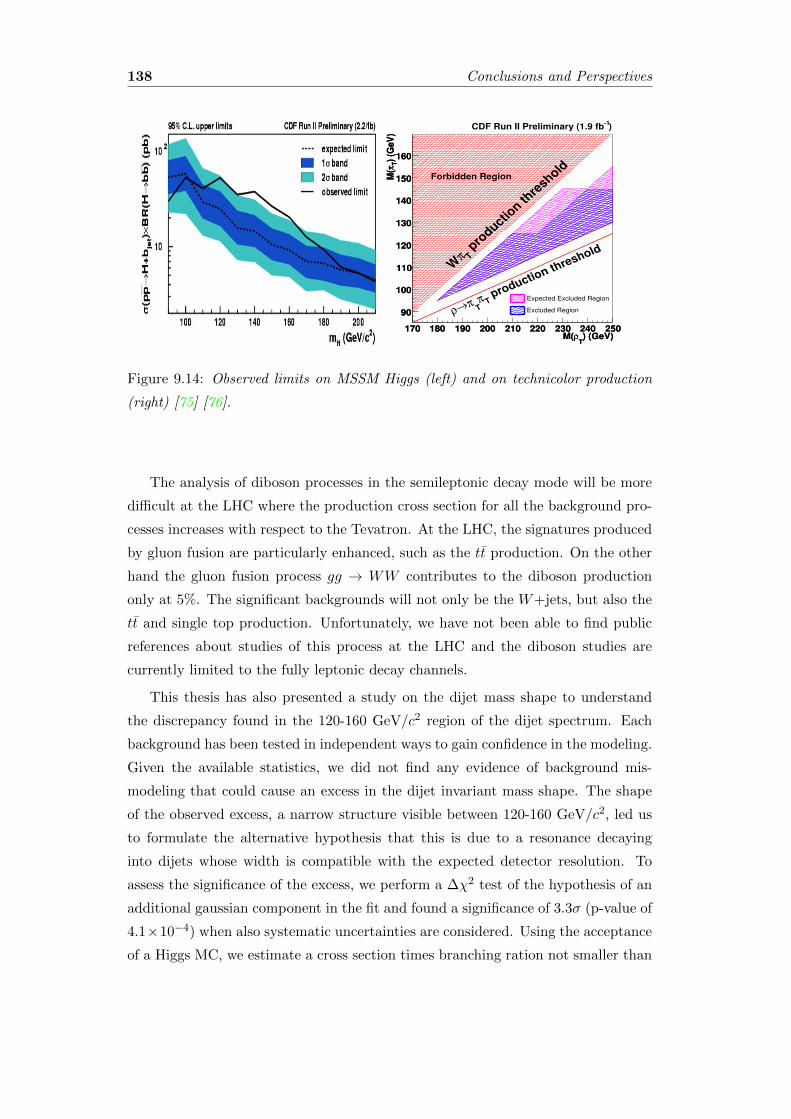
138 Conclusions and Perspectives
) (GeV)T
ρM(170 180 190 200 210 220 230 240 250
) (G
eV
)T
πM
(
90
100
110
120
130
140
150
160
) (GeV)T
ρM(170 180 190 200 210 220 230 240 250
) (G
eV
)T
πM
(
90
100
110
120
130
140
150
160
pro
ductio
n thre
shold
TπW
production th
reshold
TπTπ
→ρ
Forbidden Region
)-1
CDF Run II Preliminary (1.9 fb
Expected Excluded Region
Excluded Region
Figure 9.14: Observed limits on MSSM Higgs (left) and on technicolor production
(right) [75] [76].
The analysis of diboson processes in the semileptonic decay mode will be more
difficult at the LHC where the production cross section for all the background pro-
cesses increases with respect to the Tevatron. At the LHC, the signatures produced
by gluon fusion are particularly enhanced, such as the tt production. On the other
hand the gluon fusion process gg → WW contributes to the diboson production
only at 5%. The significant backgrounds will not only be the W+jets, but also the
tt and single top production. Unfortunately, we have not been able to find public
references about studies of this process at the LHC and the diboson studies are
currently limited to the fully leptonic decay channels.
This thesis has also presented a study on the dijet mass shape to understand
the discrepancy found in the 120-160 GeV/c2 region of the dijet spectrum. Each
background has been tested in independent ways to gain confidence in the modeling.
Given the available statistics, we did not find any evidence of background mis-
modeling that could cause an excess in the dijet invariant mass shape. The shape
of the observed excess, a narrow structure visible between 120-160 GeV/c2, led us
to formulate the alternative hypothesis that this is due to a resonance decaying
into dijets whose width is compatible with the expected detector resolution. To
assess the significance of the excess, we perform a ∆χ2 test of the hypothesis of an
additional gaussian component in the fit and found a significance of 3.3σ (p-value of
4.1×10⁻⁴) when also systematic uncertainties are considered. Using the acceptance
of a Higgs MC, we estimate a cross section times branching ration not smaller than
139
∼ 1 pb, two orders of magnitude larger that the SM Higgs. Therefore, we exclude
that the excess could be due to SM Higgs production. While we cannot exclude that
the excess is a statistical fluctuation at 3σ level or it is due to systematics being
larger than estimated, if we interpret the discrepancy as a hint of new physics,
many possibilities are still open. For example, the limits set on technicolor, ρT and
πT , production and MSSM Higgs (Fig. 9.14) do not exclude the phase space region
corresponding to our excess. It is also necessary to perform the same analysis with
the addition of b-jets tagging information, in order to gain knowledge about the
properties of the excess and the corresponding heavy flavor content. Finally, it is
critical to repeat the study described here with additional integrated luminosity to
check whether or not the excess is still in place and to perform stringent tests of
our background model that are currently limited by statistics.

140 Conclusions and Perspectives

Appendices
141

Appendix A
Lepton Trigger and
Reconstruction efficiency
A.1 Lepton Trigger Efficiency
The probability for a given event to fire a particular trigger can be parameterized in
terms of various quantities including run number, calorimeter deposit η, and track
pT . These trigger probabilities are computed by the CDF Joint Physics Group [77].
The standard method adopted by CDF to measure the high pT electron trigger
efficiency exploits an unbiased data sample, acquired with an independent trig-
ger. The trigger ELECTRON CENTRAL18, used for the present analysis, exploits both
tracking and calorimetric information, and the corresponding contributions to the
trigger efficiency can be evaluated separately [69]. The tracking efficiency can be
evaluated in a data sample acquired with a trigger path which implements the same
calorimeter requests of the ELECTRON CENTRAL18, and has no requests on tracking
quantities. The calorimetric efficiency can be evaluated in the tight electrons sam-
ple acquired in an independent trigger. Due to the structure of the tower clustering
algorithm implemented in the level 2 of this trigger path, the calorimetric efficiency
is a function of the electron transverse energy and it has been evaluated for each
period of data. The average trigger efficiency (εtrigger) for all the periods used in
this analysis is approximately 98% for an electron of 25 GeV of energy.
The procedure used by CDF collaboration to evaluate the trigger efficiency of
the high pT muon triggers is based on a very pure Z → µµ. These events are iden-
tified through the reconstruction of a pair of identified CMUP or CMX muons with
invariant mass in a narrow window around the Z mass (76 - 106 GeV/c2), and with
143
144 Appendix A. Lepton Trigger and Reconstruction efficiency
|z10 − z2
0 | < 4 cm. Furthermore at least one muon must satisfy the trigger requests.
The other muon is then exploited for the evaluation of the trigger efficiencies for
the high-pT trigger paths. In the case of muons, average trigger efficiencies have
been used, for the small variation of this value according to data periods. It value
is 89% for CMUP and assumes two different values for cmx in case the muon has
been detected by Miniskirt or Keystone subdetectors, 87% and 93% respectively
(see Sec. 2.3.6).
A.2 Electron Reconstruction Efficiency
The procedure used by CDF collaboration to evaluate the efficiency of the CEM
electrons is based on a very pure Z → e+e− sample. These events are identified
through the reconstruction of a pair of candidate electrons with invariant mass in a
narrow window around the Z mass (76−106 GeV/c2), with the first one is triggered
and satisfies tight identification cuts. The second electron is then exploited for the
evaluation of the reconstruction efficiencies for the different set of cuts.
Any disagreement between data and MC simulation can reflect in a different
value of the selection efficiencies. The standard correction procedure adopted by
the CDF collaboration relies on the evaluation of scale factors (SF) to reconcile the
reconstruction efficiencies measured in MC simulation with the ones measured in
data samples:
SFreco =εData
εMC(A.1)
This scale factors are evaluated for non-overlapping categories, therefore the tight
electrons are removed from the loose sample and the SF are calculated for each
period.
Only the scale factor is needed for this analysis, since the reconstruction effi-
ciency is obtained applying the analysis cuts on mc samples after correcting for
the scale factor to make reliable the mc estimate. The average scale factor on
reconstruction efficiency that is applied for this analysis is 98%.
A.3 Muon Reconstruction Efficiency
As in the case of electrons, reconstruction efficiencies are evaluated on pure Z →µ+µ− sample either from data or MC. The events are identified through the re-
construction of a pair of identified muons with invariant mass in a narrow window
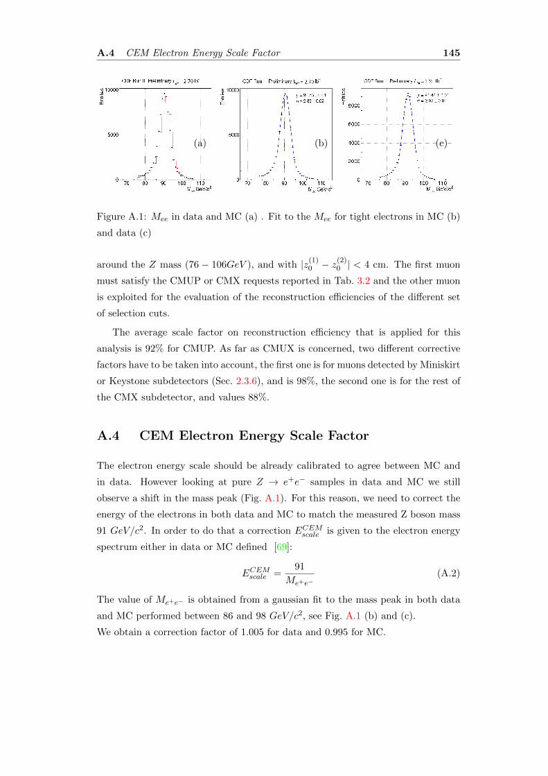
A.4 CEM Electron Energy Scale Factor 145
(a) (b) (c)
Figure A.1: Mee in data and MC (a) . Fit to the Mee for tight electrons in MC (b)
and data (c)
around the Z mass (76 − 106GeV ), and with |z(1)0 − z(2)
0 | < 4 cm. The first muon
must satisfy the CMUP or CMX requests reported in Tab. 3.2 and the other muon
is exploited for the evaluation of the reconstruction efficiencies of the different set
of selection cuts.
The average scale factor on reconstruction efficiency that is applied for this
analysis is 92% for CMUP. As far as CMUX is concerned, two different corrective
factors have to be taken into account, the first one is for muons detected by Miniskirt
or Keystone subdetectors (Sec. 2.3.6), and is 98%, the second one is for the rest of
the CMX subdetector, and values 88%.
A.4 CEM Electron Energy Scale Factor
The electron energy scale should be already calibrated to agree between MC and
in data. However looking at pure Z → e+e− samples in data and MC we still
observe a shift in the mass peak (Fig. A.1). For this reason, we need to correct the
energy of the electrons in both data and MC to match the measured Z boson mass
91 GeV/c2. In order to do that a correction ECEMscale is given to the electron energy
spectrum either in data or MC defined [69]:
ECEMscale =91
Me+e−(A.2)
The value of Me+e− is obtained from a gaussian fit to the mass peak in both data
and MC performed between 86 and 98 GeV/c2, see Fig. A.1 (b) and (c).
We obtain a correction factor of 1.005 for data and 0.995 for MC.

146 Appendix A. Lepton Trigger and Reconstruction efficiency
Appendix B
Monte Carlo Simulation
The interpretation of the data from high energy physics particle colliders and their
use to extract measurements on fundamental physical parameters often heavily relies
on the theoretical modeling of the physical processes and detailed simulation of the
interactions of particles with detectors. We refer to this as Monte Carlo since
the current knowledge of QCD and electroweak interactions is implemented using
numerical MC techniques. In recent years, a number of tools have been developed
to enable an increasingly more precise description of the final states resulting from
high energy collisions.
The main goal of a MC event generator is to provide a complete picture of the
large multiplicity of particles as the outcome of an hard interaction, whether it is
a simple scattering at large angle of some of the hadron’s elementary constituents
or their annihilation into resonances or a combination of the two. It is required to
provide the description of the particles types and momenta on an event-by-event
basis.
The fundamental idea behind the simulation of hadron-hadron collisions is the
“factorization”, the possibility of splitting the overall collision into separate and
sequential phases, approximately independent. In particular, factorization allows
to decouple the complexity of the proton structure and of the final state hadrons
formation from the elementary hard interaction among parton constituents. In
other terms, the proton structure, made of valence quarks that are held together
by a continuos exchange of gluons; the hard interaction between the constituents
of the proton and antiproton that collide, and the hadronization of the final quarks
to be bound into color neutral states, are treated as 3 well separated steps of the
whole interaction.
147
148 Appendix B. Monte Carlo Simulation
This is possible since, given Q as the scale of the the hard interaction, its time
frame is so short ( 1Q) that the interaction of the quark involved in the scattering
with the rest of the quarks can be neglected, being impossible for the struck quark
to negotiate with its partners a coherent response to the external perturbation,
while it is kicked away. After the interaction, the final partons get through a phase
in which they emit radiation until an exchange equilibrium is reached again and
the memory of the hard process has been lost. At this moment, the hadronization
process takes over, nearby partons merge into color singlets and the initial hadrons
fragments are recombined leading to the underlying event final states.
The Monte Carlo generators can be divided into two main cathegories:
1 Parton-Level generators
2 Parton-Shower generators
B.1 Parton Distribution Function
A given physics process at a hadron collider begins with two quarks or gluons in the
initial state. These quarks and gluons come from protons and antiprotons, either
as valence quarks or extracted from the sea of virtual particles. The momentum
distribution of the constituent partons (a general term which includes quarks and
gluons) in a proton is given by parton distribution functions (PDFs).
PDFs are determined for each flavor of quark and antiquark, as well as for
gluons,in a proton. They give the probability density for finding a parton with a
given fraction of longitudinal momentum in an interaction with a given momentum
transfer Q2.
These parameterize the longitudinal momenta of different types of quarks and
gluons within the proton as a function of the momentum transfer of the collision. An
event generator starts with a pair of partons with a certain momentum, and assigns
weights to each event based on the PDFs. Because they rely on non-perturbative
QCD effects, PDFs require input from experimental data. The CTEQ5L PDFs are
used in generating all MC samples in this analysis [72].
B.2 Event Generation
The calculation of a hard scattering process is based on tree-level Feynman diagrams
and is, in many cases, straightforward. In most cases, the simplest leading-order
B.2 Event Generation 149
diagram is calculated as a hard scattering process and radiated leptons, photons, or
gluons are treated by a showering algorithm. Next-to-leading-order MC generators
are starting to become available, but have not yet been sufficiently validated on
CDF data to use in this analysis.
A MC generator uses an ”unweighting” method to simulate the relative rate of
different event kinematics. First, it creates a large number of events with randomly
assigned kinematic properties. It calculates a weight for each event based on the
differential cross section for the event, and its kinematic properties. Then it converts
each weight to a probability, taking the highest weight to be unity. This gives the
relative contribution of each region of phase space.
The generator then examines each event again, choosing a random number be-
tween 0 and 1 for each event and keeping only events for which the random number
is less than the probability for that event. This results in a set of discrete, unit-
weight events whose kinematics, for a large number of events, properly reflects the
differential cross section of the process. In this analysis, the MC simulated samples
of events are produced using three different generators:
• PYTHIA to generate WW and WZ events (signal) and tt production.
• MADEVENT to generate single top production .
• ALPGEN to generate Z+jets and W+jets production.
B.2.1 PYTHIA
PYTHIA [60] [78] is a program realized to describe the collision between elementary
particles (leptons, quark and vector bosons). It is able to describe low energy and
high energy interactions, partonic distribution, initial and final states of hadronic
showers, multiple interaction, fragmentation and decays. The goal is to provide the
most accurate description of the event in a wide range of interaction with emphasis
for the strong interactions. For the time being we don’t have a methodology that is
able to give an exact description of physical processes ruled by the strong interaction:
PYTHIA processes are then based on a combination of analytical results and various
QCD models.
The advantage of PYTHIA is its speed and its ability to generate an arbitrarily
large number of jets without needing to recalculate matrix elements. On the other
hand, it works only as an approximation and lacks color flow information from
150 Appendix B. Monte Carlo Simulation
the matrix elements. However, color flow is not a major concern for electroweak
processes because they have only one gluon in next-to-leading-order diagrams; only
for diagrams with many gluons is it a major concern, requiring ALPGEN for a proper
calculation.
B.2.2 MADEVENT
MADEVENT [79] is a MC generator that can calculate arbitrary tree-level diagrams
with full color and spin polarization information included.MADEVENT is powered by
the matrix element generator MADGRAPH [80]. Given a SM process, MADGRAPH auto-
matically generates the amplitudes for all relevant sub-processes and produces the
mappings for the integration over the phase space. This process dependent infor-
mation is passed to MADEVENT and a stand-alone code is produced that allows the
user to calculate cross sections and to obtain unweighted events. Once the events
have been generated, they may be passed to showering MC programs.
B.2.3 ALPGEN
Processes with an electroweak boson and radiated gluons are difficult to deal with,
because of the large amount of radiation they produce; the showering approximation
used by PYTHIA, being based only on the tree-level diagram, does not include effects
of color flow. However, a full calculation of the matrix elements involved is difficult
because the number of distinct diagrams grows as the factorial of the number of
jets.
ALPGEN [15] is a MC generator designed specifically for processes whose final
state contains an electroweak boson and several radiated quarks and gluons, a ma-
jor background this analysis. ALPGEN calculates the matrix elements for processes
with gluon radiation and passes the color information to the showering algorithm.
This should give a more accurate modeling of the kinematics of the process than
PYTHIA’s showering approximation, since it includes proper matrix element cal-
culations of the event. ALPGEN also calculates the leading-order cross section of
each interaction it generates, which is useful for combining different processes.
B.3 Showering
All events, regardless of how they were generated, are passed to PYTHIA for parton
showering and hadronization. The showering procedure generates initial and final
B.4 Dector simulation 151
state gluon radiation for each event and allows them to decay to quark pairs, in-
creasing the number of particles in the final state of the event. More particles may
be added from effects of beam remnants or multiple interactions. This gives the
final set of particles that are passed to the hadronization routine.
Since the hadronization of quarks and gluons, which describes the formation of
jets, takes place at low Q2 and large αs, perturbation theory cannot be applied.
The phenomenologic models, used to describe hadronization in the absence of any
firm theoretical understanding are different for distinct MC generators. PYTHIA
performs its hadronization using the Lund color string model. Each pair of quarks
is modeled as though connected by a relativistic string which increases linearly in
energy as separation increases. As the energy in the string increases, it becomes
increasingly more probable that it will form a new quark-antiquark pair. These new
particles can then be grouped with the original ones to form mesons and baryons.
Most of the particles resulting from hadronization are unstable, so PYTHIAcauses
them to decay into relatively stable particles (electrons and muons, protons and
neutrons, pions and kaons) that can actually be detected. This step uses branching
ratios and lifetimes measured in various experiments to calculate the final decay
products. In this procedure, PYTHIA ignores spin information and uses a simplified
algorithm for B mesons and tau leptons.
B.4 Dector simulation
Once the final long-lived particles have been generated, it is important to determine
how the detector will respond to them. This requires a full detector simulation
which simulates the response of the different subcomponents of the detector, in-
cluding resolution effects, inherent inefficiencies in the detector, and the behavior of
the particles as they pass through passive material (such as cables or support struc-
tures) in the detector. When this is done, the MC events can be put into a data
structure identical to that obtained from collision data, thus allowing reconstruction
algorithms to work exactly the same way on data and MC events.
CDF uses a program called GEANT [81] to model the tracking volume of the
detector. GEANT allows the construction of a mathematical model of the detector
which can simulate the passage of charged particles through it, including showering
to secondary or tertiary particles. This is used along with charge deposition mod-
els to simulate the response of the tracking detectors (silicon and COT). Because
modeling the interactions of each particle and all its secondary particles is computa-

152 Appendix B. Monte Carlo Simulation
tionally intensive, CDF stops using GEANT after the first inelastic collision occurs in
the calorimeter. Instead it switches to a parameterized calorimeter response, tuned
to test beam data, which employs a program called GFLASH [82]. This rapidly and
accurately simulates the response of the calorimeter towers to the energy deposited
by the incoming charged particles, completing the detector simulation.
Bibliography
[1] T. Aaltonen et al. (CDF Collaboration), “Measurement of the WW + WZ
Production Cross Section Using the Lepton + Jets Final State at CDF II”,
Phys. Rev. Lett. 104 (2010) 101801.
[2] V. Cavaliere for the CDF Collaboration,“Diboson Production (CDF)”,
PoS(EPS-HEP2009)347; T. Aaltonen et al. (CDF Collaboration), “Measure-
ment of WW/WZ Cross Section in `νjj Decay Using 4.3 fb−1”, CDF Public
Webpage.
[3] M. Peskin and D. Schroeder, “An Introduction to Quantum Field Theory”,
Westview Press 1995.
[4] M. Goldhaber, L. Grodzins and A. W. Sunyar, “Helicity of Neutrinos”, Phys.
Rev. Lett. 109 (1958) 1015.
[5] K. Nakamura et al. (Particle Data Group), J. Phys. G 37 (2010) 075021.
[6] S. L. Glashow, “Partial Symmetries of Weak Interactions”, Nucl. Phys. A 22
(1961) 579; S. Weinberg, “A Model of Leptons”, Phys. Rev. Lett. 19 (1967)
1264; A. Salam, “Elementary Particle Theory”, ed. by N. Svartholm (Almqvist
and Wiksells, Stockholm, 1968).
[7] P. W. Higgs, “Broken Symmetries, Massless Particles And Gauge Fields”, Phys.
Rev. Lett. 12 (1964) 132; P. W. Higgs, “Broken Symmetries And The Masses
Of Gauge Bosons”, Phys. Rev. Lett. 13 (1964) 508.
[8] LEP Working Group for Higgs Boson Searches (ALEPH, DELPHI, L3, and
OPAL), “Search for the Standard Model Higgs Boson at LEP”, Phys. Rev.
B 565 (2003) 61; CDF and DØ Collaborations, “Combination of Tevatron
Searches for the Standard Model Higgs Boson in the WW Decay Mode”, Phys.
Rev. Lett. 104 (2010) 061802.
153
154 Bibliography
[9] Johannes Haller (Gfitter group), “The electroweak fit and constraints on new
physics”, [arXiv:1006.0003v1].
[10] M. C. Gonzalez-Garcia and Y. Nir, “Neutrino Masses and Mixing: Evidence
and Implications”, Rev. Mod. Phys. 75 (2003) 345-402.
[11] H. Georgi, H. R. Quinn and S. Weinberg, “Hierarchy of Interactions in Unified
Gauge Theories”, Phys. Rev. Lett. 33 (1974) 451; L. Susskind, “Dynamics of
Spontaneous Symmetry Breaking in the Weinberg-Salam Theory”, Phys. Rev.
D 20 (1979) 2619.
[12] J. Polchinski and L. Susskind, “Breaking of Supersymmetry at Intermediate
Energy”, Phys. Rev. D 26 (1982) 3661.
[13] C. T. Hill and E. H. Simmons, “Strong Dynamics and Electroweak Symmetry
Breaking”, Phys. Rept. 381 (2003) 235402 [arXiv:hep-ph/0203079].
[14] J. M. Campbell and R. K. Ellis, “Update on Vector Boson Pair Production at
Hadron Colliders”, Phys. Rev. D 60 (1999) 113006.
[15] M. L. Mangano et al., “ALPGEN, a Generator for Hard Multiparton Processes
in Hadronic Collisions”, J. High Energy Phys. 07 (2003) 001 [arXiv:hep-
ph/0206293].
[16] P. Mastrandrea for the CDF and DØ Collaborations, “Multi-Boson Produc-
tion”, FERMILAB-CONF-09-754-PPD, 2010.
[17] M. Carena, S. Heinemeyer, C. E. M. Wagner and G. Weiglein, “Suggestions for
Benchmark Scenarios for MSSM Higgs Boson Searches at Hadron Colliders”,
Eur. Phys. J. C 26 (2003) 601 [arXiv:hep-ph/0202167].
[18] M. Carena, S. Mrenna and C. E. M. Wagner, “MSSM Higgs Boson Phenomenol-
ogy at the Tevatron Collider”, Phys. Rev. D 60 (1999) 075010.
[19] The LEP Collaborations, “A Combination of Preliminary Electroweak Mea-
surements and Constraints on the Standard Model”, [arXiv:hep-ex/0511027].
[20] V. Abazov et al. (DØ Collaboration), “Measurement of the WW Production
Cross Section with Dilepton Final States in pp Collisions at√s = 1.96 TeV
and Limits on Anomalous Trilinear Gauge Couplings”, Phys. Rev. Lett. 103
(2009) 191801.
Bibliography 155
[21] CDF Collaboration, “Measurement of the WW Production Cross Section in
pp Collisions at√s = 1.96 TeV Using 3.6 fb−1 of CDF Run II Data”, Phys.
Rev. Lett. 104 (2010) 201801.
[22] V. Abazov et al. (DØ Collaboration), “Measurement of the pp→WZ+X Cross
Section at√s = 1.96 TeV and Limits on WWZ Trilinear Gauge Couplings”,
Phys. Rev. D 76 (2007) 111104.
[23] T. Aaltonen et al. (CDF Collaboration), “Measurement of the WZ and ZZ
Production Cross Sections Using WZ → 3` +��ET and ZZ → 4` Channels”,
CDF Note 10238.
[24] T. Aaltonen et al. (CDF Collaboration), “First Observation of Vector Boson
Pairs in a Hadronic Final State at the Tevatron Collider”, Phys. Rev. Lett. 103
(2009) 091803.
[25] V. M. Abazov et al. (DØ Collaboration), “Evidence of WW +WZ Production
with Lepton+Jets Final States in Proton-Antiproton Collisions at√s = 1.96
TeV”, Phys. Rev. Lett. 102 (2009) 161801.
[26] T. Aaltonen et al. (CDF Collaboration), “Measurement of WW + WZ Pro-
duction Cross Section in `νjj Channel in L = 4.6 fb−1 of CDF Run II Data
Using a Matrix Element Technique”, CDF Public Webpage.
[27] Fermilab Beam Division, “Run II Handbook”, http://www-bd.fnal.gov.
[28] C. S. Hill et al. (CDF Collaboration), “Operational Experience and Perfor-
mance of the CDF II Silicon Detector”, Nucl. Instrum. Meth. A530 (2004)
1.
[29] A. Still et al. (CDF Collaboration), “SVX-II: CDF Run II Silicon Tracking
Projects”, Nucl. Instrum. Meth. A447 (2000) 1.
[30] B. Ashmanskas et al. (CDF Collaboration), “The CDF Silicon Vertex Trigger”,
Nucl. Instrum. Meth. A518 (2004) 532 [arXiv:physics/0306169]; I. Vila for
the CDF Collaboration, “Performance and First Physics Results of the SVT
Trigger at CDF II”, ECONF C0304052:FO008, 2003 [arXiv:hep-ph/0307165].
[31] J. A. Adelam et al. (CDF Collaboration), “The Silicon Vertex Trigger Upgrade
at CDF”, Nucl. Instrum. Meth. A572 (2007) 361; S. Amerio et al., “The Gi-
gaFitter: Performance at CDF and Perspectives for Future Applications”, J.
Phys. Conf. Ser. 219 022001 [doi:10.1088/1742-6596/219/2/022001].
156 Bibliography
[32] T. Affolder et al. (CDF Collaboration), “COT Central Outer Tracker”, Nucl.
Instrum. Meth. A526 (2004) 249.
[33] See CDF Run II Detector Parameters, COT Simulation Validation Plots.
[34] D. Acosta et al. (CDF Collaboration), “A Time-Of-Flight Detector in CDF II”,
Nucl. Instrum. Meth. A518 (2004) 605.
[35] L. Balka et al. (CDF Collaboration), “The CDF Central Electromagnetic
Calorimeter”, Nucl. Instrum. Meth. A267 (1988) 272.
[36] S. Bertolucci et al. (CDF Collaboration), “The CDF Central and Endwall
Hadron Calorimeter”, Nucl. Instrum. Meth. A267 (1988) 301.
[37] M. Albrow et al. (CDF Collaboration), “The CDF Plug Upgrade Electromag-
netic Calorimeter: Test Beam Results”, Nucl. Instrum. Meth. A480 (2002)
524.
[38] M. Gallinaro et al. (CDF Collaboration), “A New Scintillator Tile/Fiber
Preshower Detector for the CDF Central Calorimeter”, IEEE Trans. Nucl. Sci.
52, 2005 (879) [arXiv:physics/0411056]; M. Albrow et al. (CDF Collaboration),
“A preshower detector for the CDF Plug Upgrade: Test Beam Results”, Nucl.
Instrum. Meth. A431 (1999) 104; G. Apollinari et al. (CDF Collaboration),
“Shower maximum detector for the CDF plug upgrade calorimeter”, Nucl. In-
strum. Meth. A412 (1998) 515.
[39] G. Ascoli et al. (CDF Collaboration), “CDF central muon detector”, Nucl.
Instrum. Meth. A268 (1988) 33.
[40] K. Byrum et al. (CDF Collaboration), “The CDF forward muon system”, Nucl.
Instrum. Meth. A268 (1988) 46.
[41] CDF Collaboration, “The CDF II Detector-Technical Design Report”, 1996
FERMILAB-Pub-96/390-E CDF.
[42] D. Acosta et al. (CDF Collaboration), “The CDF Luminosity Monitor”, Nucl.
Instrum. Meth. A461 (2001) 540.
[43] S. Klimenko J. Konigsberg and T. Liss, “Averaging of the inelastic cross sec-
tions measured by the CDF and the E811 experiments”, Fermilab-FN-0741
(2003).
Bibliography 157
[44] D. Acosta et al. (CDF Collaboration), “The Performance of the CDF Lumi-
nosity Monitor”, Nucl. Instrum. Meth. A494 (2002) 57.
[45] F. Abe et al., “Measurement of the anti-proton proton total cross section at√s = 546 GeV”, Phys. Rev. D 50 (1994) 5550.
[46] S. Klimenko, J. Konigsberg and T. Liss, “Averaging the inelastic cross-section
measured by CDF and the E811 experiments”, Fermilab-FN-0741 (2003).
[47] S. Jindariani et al., “Luminosity Uncertainty for Run 2 up until August 2004”,
CDF Note 7446
[48] A. Canepa et al., “Level-3 Calorimetric Resolution available for the Level-1
and Level-2 CDF Triggers”, [arXiv:0810.3738].
[49] The Trigger and Datasets Working Group, “Run II Trigger Table and Datasets
Plan”, CDF Note 4718.
[50] P. Azzi at al., “Histogram Tracking in the COT”, CDF Note 5562.
[51] F. D. Snider (CDF Collaboration), “Tracking at CDF: Algorithms and experi-
ence from Run I and Run II”, Nucl. Instrum. Meth. A566 (2006) 133.
[52] C. P. Hays et al., “Inside-out tracking at CDF”, Nucl. Instrum. Meth. A538
(2005) 249.
[53] J. Goldstein at al., “Silicon Tracking for Plug Electrons”, CDF Note 5970.
[54] A. Abulencia et al. (CDF Collaboration), “Measurements of Inclusive W and
Z Cross Sections in pp Collisions at√s = 1.96 TeV”, J. Phys. G: Nucl. Part.
Phys. 34 (2007) 2457 [doi:10.1088/0954-3899/34/12/001].
[55] D. Acosta et al. (CDF Collaboration), “Direct Photon Cross Section with Con-
versions at CDF”, Phys. Rev. D 70 (2004) 074008.
[56] A. Taffard, “Run II Cosmic Ray Tagger Performances”, CDF Note 6255.
[57] E. Lipeles et al., “Lepton ID for Multilepton Diboson Analyses”, CDF Note
8538.
[58] F. Abe et al. (CDF Collaboration), “The Topology of Three Jet Events in pp
Collisions at√s = 1.8 TeV”, Phys. Rev. D 45 (1992) 1448.
158 Bibliography
[59] A. Bhatti et al. (CDF Collaboration), “Determination of the Jet Energy Scale
at the Collider Detector at Fermilab”, Nucl. Instrum. Meth. A566 (2006) 375;
CDF Collaboration, “Generic Jet Energy Corrections at CDF”, CDF Public
WebPage
[60] T. Sjostrand et al., “High-Energy-Physics Event Generation with PYTHIA 6.1”,
Comput. Phys. Commun. 135 (2001) 238 [arXiv:hep-ph/0010017]
[61] B. Cooper and A. Messina, “Estimation of the Background to W → eν+n jets
Events”, CDF Note 7760.
[62] M. Cacciari et al., “Updated Predictions for the Total Production Cross Sec-
tions of Top and of Heavier Quark Pairs at the Tevatron and at the LHC”, J.
High Energy Phys. 0809 (2008) 127.
[63] B. W. Harris et al., “Fully Differential Single-Top-Quark Cross Section in Next-
to- Leading Order”, Phys. Rev. D 66 (2002) 054024.
[64] S. Hoche et al., “Matching Parton Showers and Matrix Elements”, [arXiv:hep-
ph/0602031v1].
[65] T. Aaltonen et al., (CDF Collaboration), “Measurement of Inclusive Jet Cross
Sections in Z/γ∗(→ e+e−)+jets Production in pp Collisions at√s=1.96 TeV”,
Phys. Rev. Lett. 100 (2008) 102001
[66] J. Adelman et al., “Method II For You”, CDF Note 9185.
[67] F. James and M. Roos, “MINUIT: A system For Function Minimization And
Analysis Of The Parameter Errors and Correlations”, Comput. Phys. Commun.
10 (1975) 343; F. James, “MINUIT: Function Minimization And Error Analysis
- Reference Manual”, CERN Program Library (1998) D506.
[68] F. Canelli et al., “Jet Energy Resolution”, CDF Note 7856.
[69] T. Spreitzer et al., “Electron Identification in Offline Release”, CDF Note 7950.
[70] ALEPH Collaboration, “Measurement of isolated photon production in
hadronic Z decays”, Phys. Rev. B 264 (1991) 3
[71] A. Abulencia et al. (CDF Collaboration), “Top Quark Mass Measurement Us-
ing the Template Method in the Lepton + Jets Channel at CDF II”, Phys.
Rev. D 73 (2006) 032003.
Bibliography 159
[72] H. L. Lai et al., “Global QCD Analysis of Parton Structure of the Nucleon:
CTEQ5 Parton Distributions”, Eur. Phys. J. C 12 (2000) 375 [arXiv:hep-
ph/9903282v3].
[73] A. D. Martin et al., “Parton Distributions and the LHC: W and Z Production”,
Eur. Phys. J. C 14 (2000) 133.
[74] L. Demortier, “P-Values and Nuisance Parameters”, Proceedings of PHYSTAT
2007, CERN-2008-001, p. 23.
[75] T. Aaltonen et al. (CDF Collaboration),“Search for Technicolor Particles Pro-
duced in Association with a W Boson at CDF”, Phys. Rev. Lett. 104 (2010)
111802
[76] CDF Collaboration, “Search for Higgs Bosons Produced in Association with
b-Quarks”, CDF Note 10105
[77] Joint Physics Group, CDF Internal Webpage.
[78] T. Sjostrand, S. Mrenna and P. Skands, “PYTHIA 6.4 physics and manual”,
J. High Energy Phys. 05 (2006) 026 [arXiv:hep-ph/0603175].
[79] F. Maltoni and T. Stelzer, “MadEvent: automatic event generation with Mad-
Graph”, J. High Energy Phys. 02 (2003) 027 [arXiv:hep-ph/0208156].
[80] T. Stelzer and W.F. Long, “Automatic generation of tree level helicity ampli-
tudes”, Comput. Phys. Commun. 81 (1994) 357 [arXiv:hep-ph/9401258].
[81] S. Agostinelli et al., Nucl. Instrum. Meth. 506 (2003) 250.
[82] GFLASH CERN Web Page

160 Bibliography

Acknowledgements
And last but not least the acknowledgements, that means that the thesis is finished!
And as always too little time to really express my gratefulness to everybody, so I
will try my best to use one of my few qualities, the synthesis.
I would like to start thanking my supervisor Agnese for always letting me choose
the things that I wanted to do, giving me the freedom of working independently,
but always taking care of me. In order then, I would like to thank Alberto and
Pierluigi, colleagues and friends, with whom I shared this adventure and the hard
work. Thanks for your help, I really appreciate it. I must also thank Luciano for
his guidance and support, especially in the life at Fermilab.
And then all the friends both in Fermilab, Pisa and Rome. You made my breaks
happier, listened to my complaints, shared snacks, laughed and cried with me. Your
name might not be here but I thank you all deeply. A big thank you goes also to
the “printing team” in Pisa, without you my thesis for sure would still be in the
mail over the atlantic ocean.
In particular I want to thank Patrizia. I couldn’t have asked for a better friend
to share this Phd, you made everything a fun experience. As I already told you the
lost page 85 is dedicated to you.
This thesis is dedicated to my family, that always supported me and believed in
me no matter the choices I took. I always love to come back home and spend time
with you.
Last I would like to thank Angelo. Not only for his practical help in every single
issue I had in the analysis and in writing the thesis, but for being my best friend
and partner in all these years and hopefully forever.
161