Lucas PlatterInstitute for Nuclear Theory

University of Washington

Universalityin

Few- and Many-Body Systems

Collaborators: Braaten, Hammer, Kang, Phillips, Ji

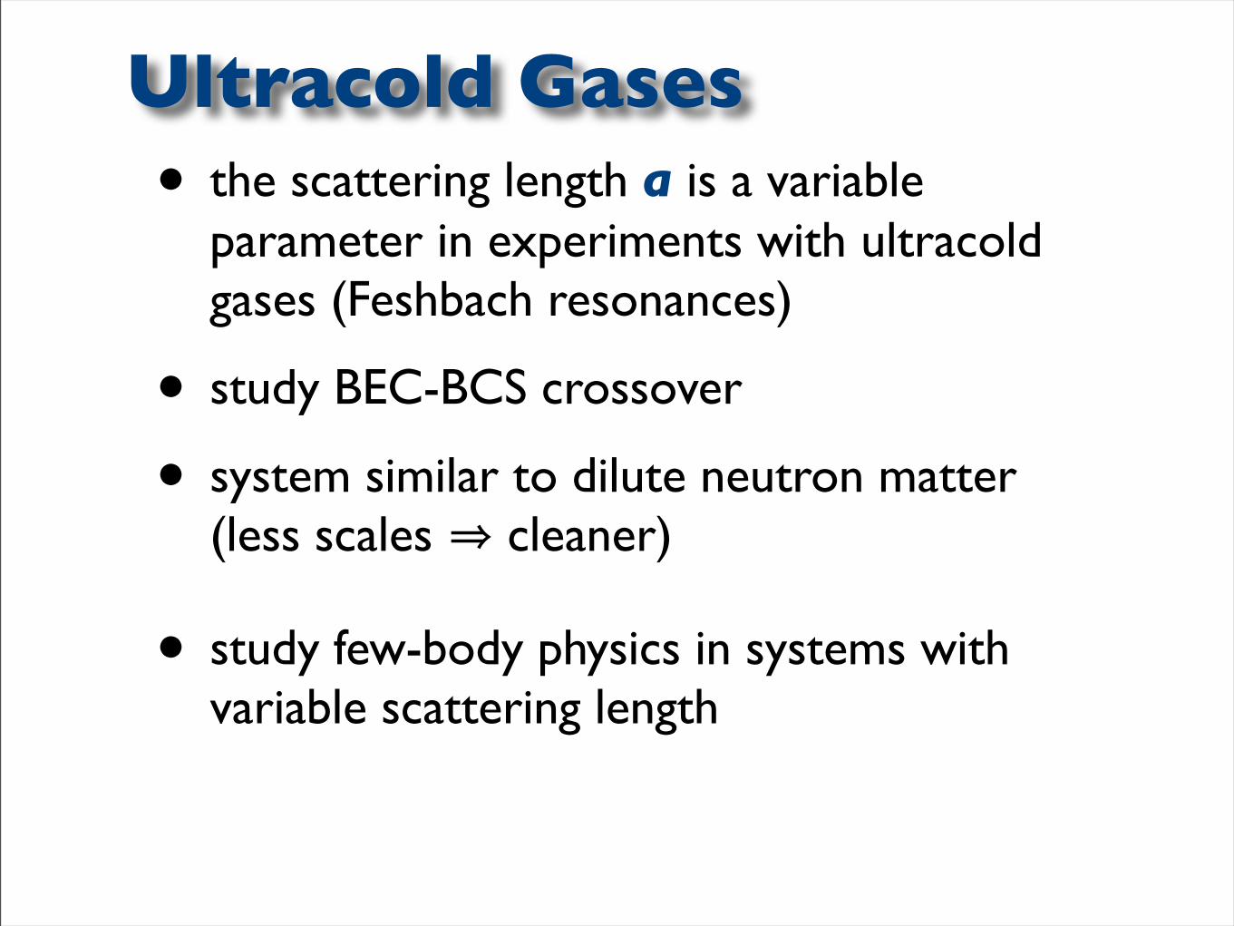
Ultracold Gases• the scattering length a is a variable

parameter in experiments with ultracold gases (Feshbach resonances)

• study BEC-BCS crossover

• system similar to dilute neutron matter (less scales ⇒ cleaner)

• study few-body physics in systems with variable scattering length

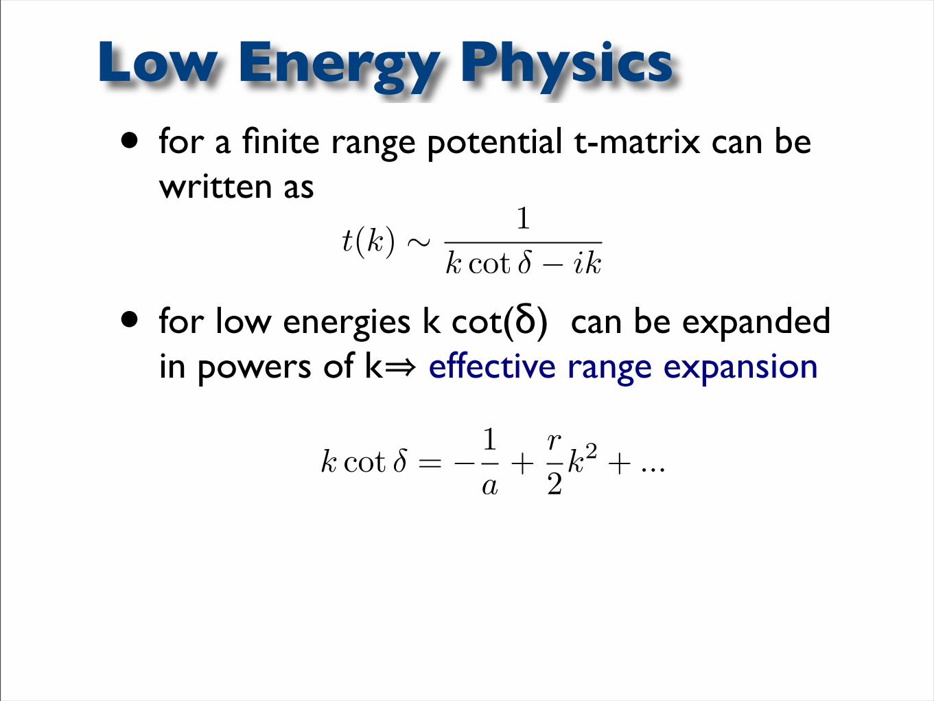
• for a finite range potential t-matrix can be written as

• for low energies k cot(δ) can be expanded in powers of k⇒ effective range expansion

Low Energy Physics

t(k) ∼ 1k cot δ − ik

k cot δ = −1a

+r

2k2 + ...

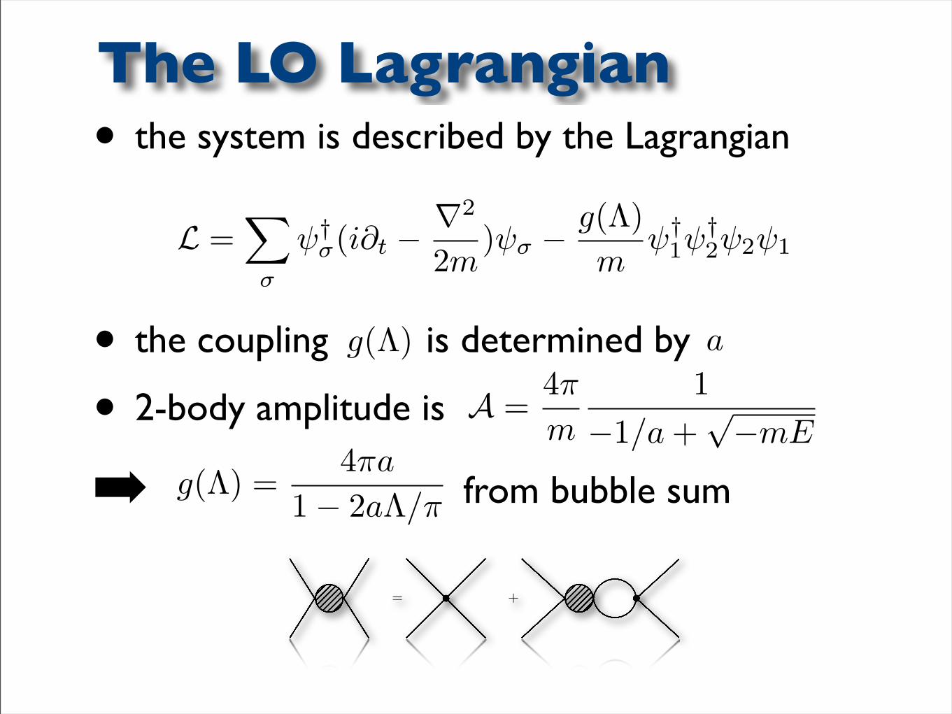
• the system is described by the Lagrangian

• the coupling is determined by

• 2-body amplitude is

from bubble sum

The LO Lagrangian

L =∑

σ

ψ†σ(i∂t −

∇2

2m)ψσ −

g(Λ)m

ψ†1ψ

†2ψ2ψ1

g(Λ) a

g(Λ) =4πa

1− 2aΛ/π

= +

A =4π

m

1−1/a +

√−mE

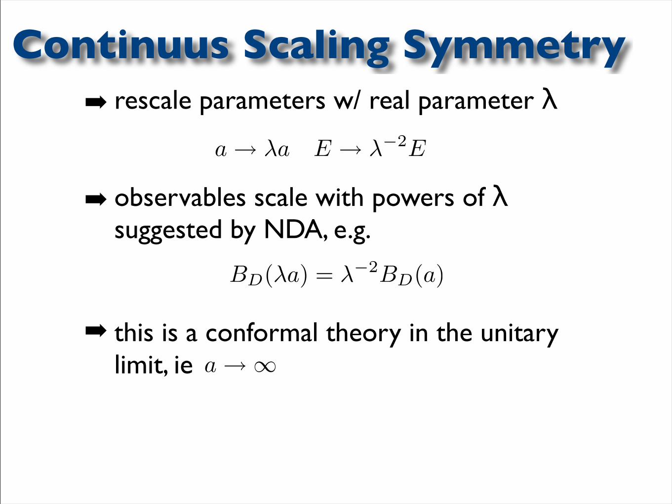
rescale parameters w/ real parameter λ

observables scale with powers of λ suggested by NDA, e.g.

this is a conformal theory in the unitary limit, ie

Continuus Scaling Symmetry

a→∞

a→ λa E → λ−2E

BD(λa) = λ−2BD(a)

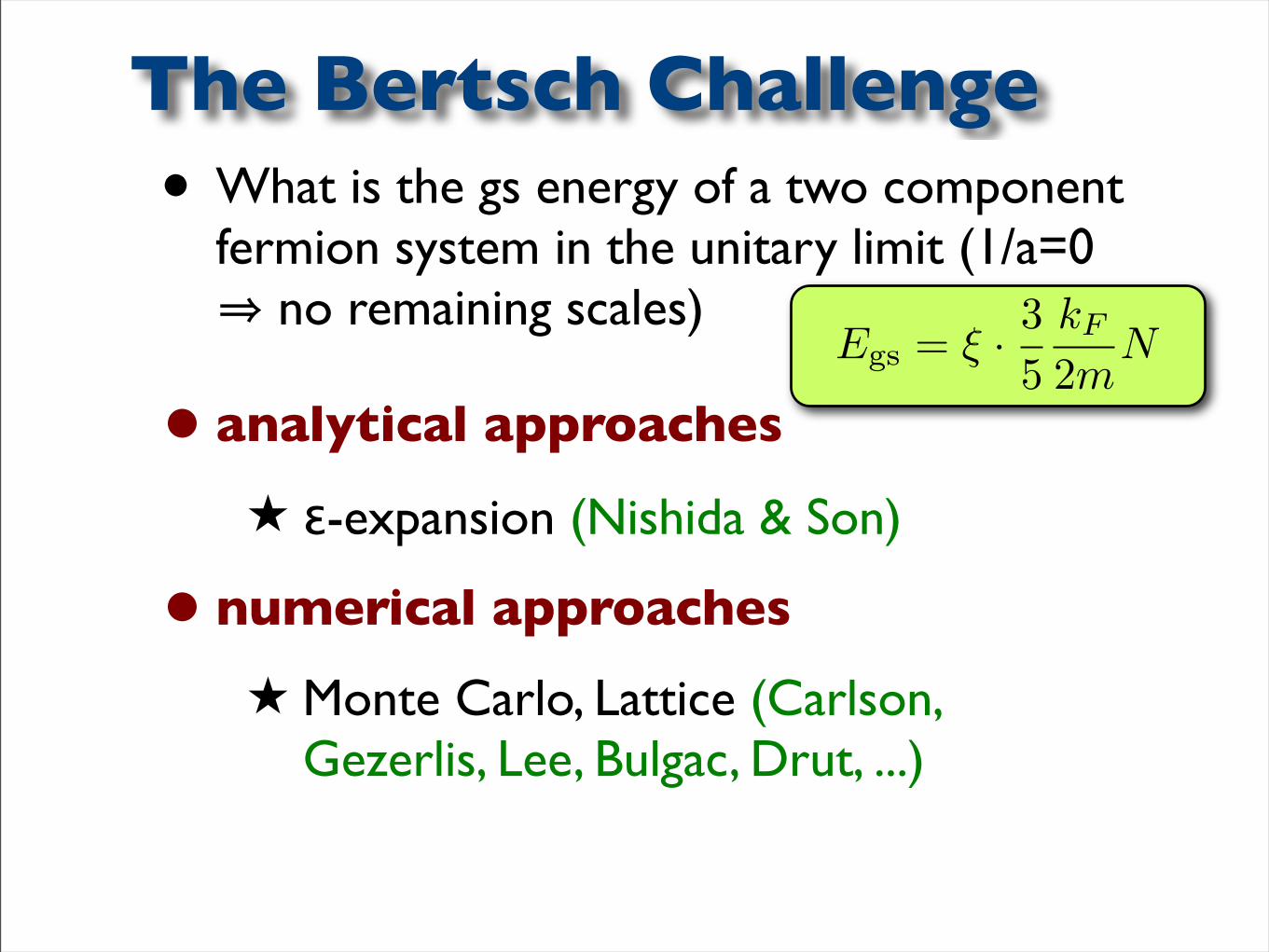
• What is the gs energy of a two component fermion system in the unitary limit (1/a=0 ⇒ no remaining scales)

• analytical approaches

ε-expansion (Nishida & Son)

• numerical approaches

Monte Carlo, Lattice (Carlson, Gezerlis, Lee, Bulgac, Drut, ...)

The Bertsch Challenge

Egs = ξ · 35

kF

2mN

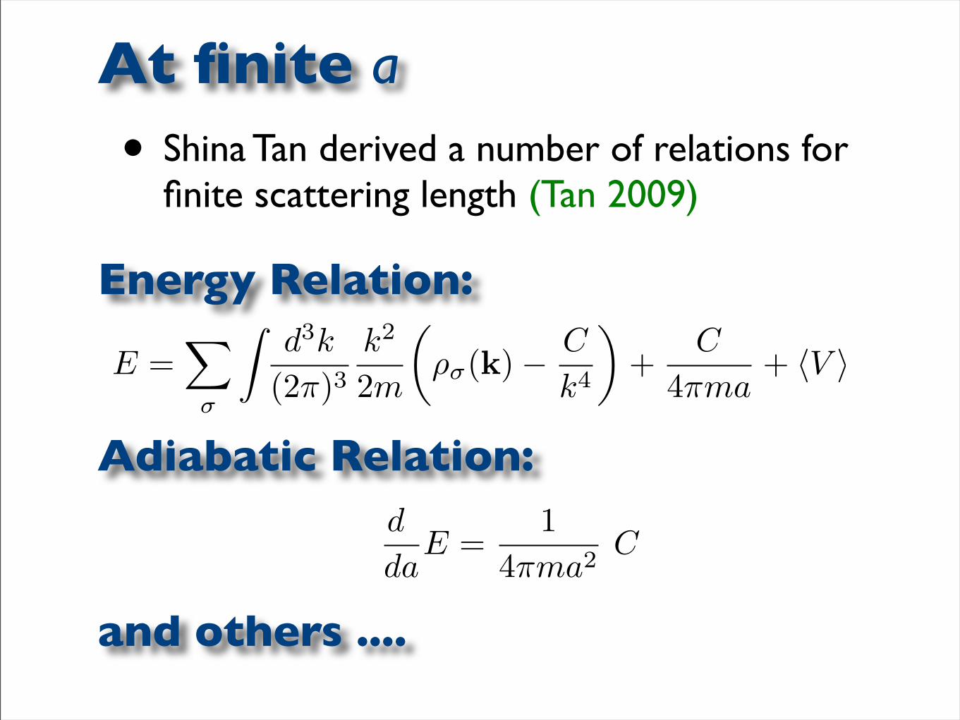
• Shina Tan derived a number of relations for finite scattering length (Tan 2009)

At finite a

Energy Relation:

E =∑

σ

∫d3k

(2π)3k2

2m

(ρσ(k) − C

k4

)+

C

4πma+ 〈V 〉

Adiabatic Relation:d

daE =

14πma2

C

and others ....

What is C?

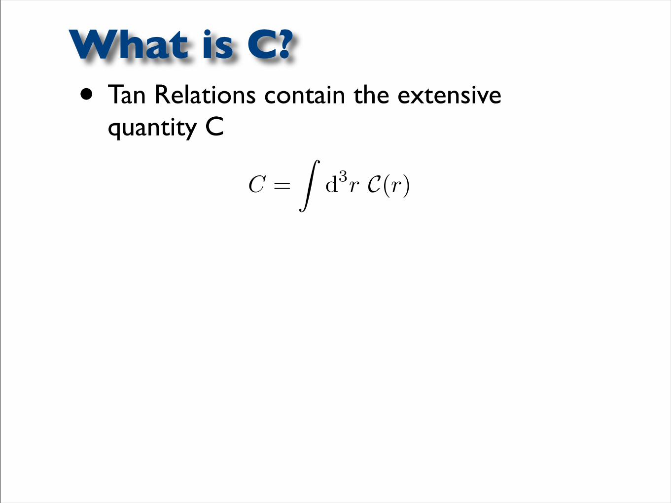
• Tan Relations contain the extensive quantity C

C =∫

d3r C(r)

What is C?

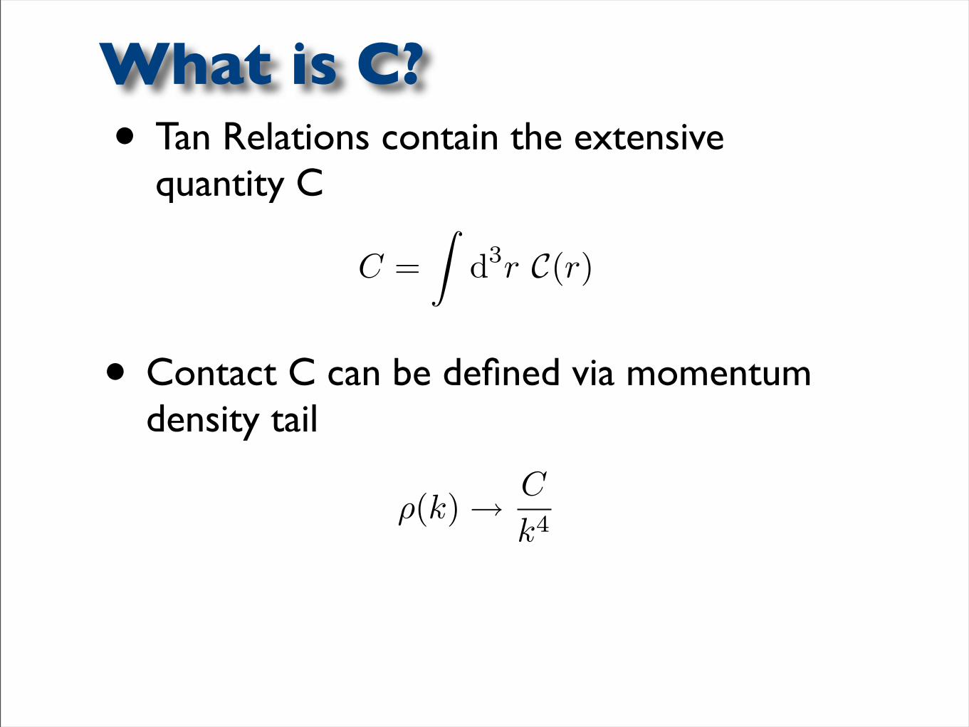
• Tan Relations contain the extensive quantity C

C =∫

d3r C(r)

ρ(k)→ C

k4

What is C?

• Contact C can be defined via momentum density tail

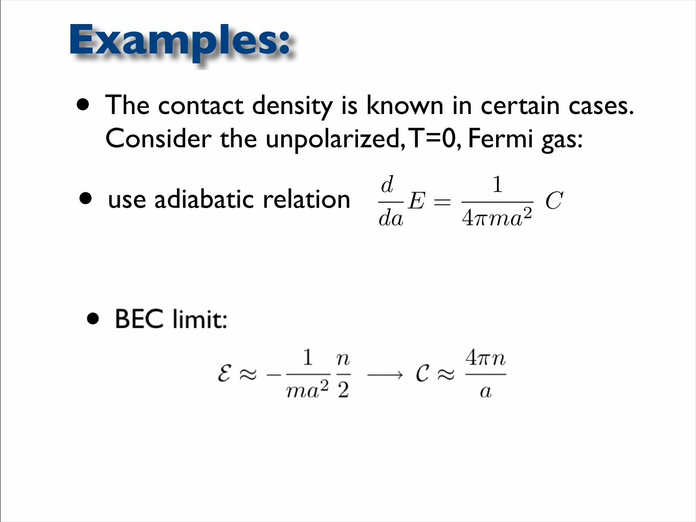
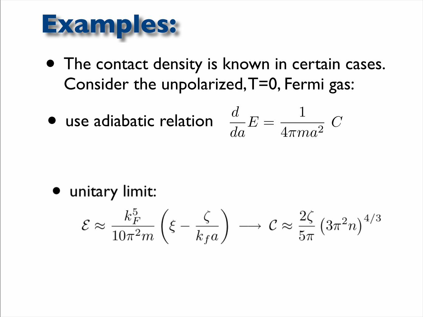
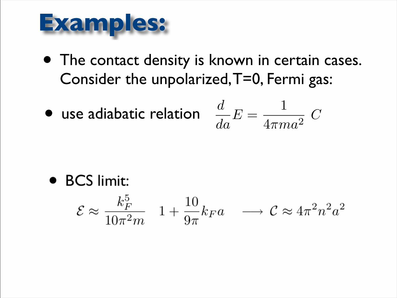
• The contact density is known in certain cases. Consider the unpolarized, T=0, Fermi gas:

Examples:

• use adiabatic relation d

daE =

14πma2

C

• The contact density is known in certain cases. Consider the unpolarized, T=0, Fermi gas:

Examples:

• use adiabatic relation d

daE =

14πma2

C

• The contact density is known in certain cases. Consider the unpolarized, T=0, Fermi gas:

Examples:

• use adiabatic relation d

daE =

14πma2

C

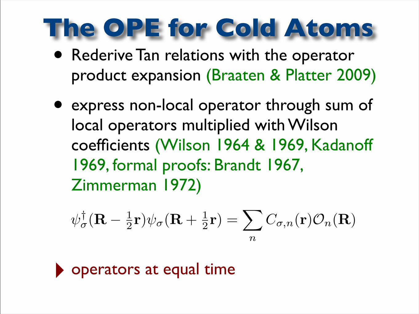
• Rederive Tan relations with the operator product expansion (Braaten & Platter 2009)

• express non-local operator through sum of local operators multiplied with Wilson coefficients (Wilson 1964 & 1969, Kadanoff 1969, formal proofs: Brandt 1967, Zimmerman 1972)

‣ operators at equal time

The OPE for Cold Atoms

ψ†σ(R− 1

2r)ψσ(R + 12r) =

∑

n

Cσ,n(r)On(R)

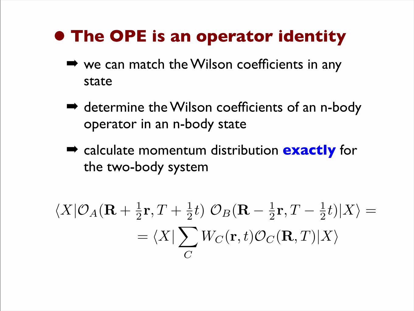
• The OPE is an operator identity

we can match the Wilson coefficients in any state

determine the Wilson coefficients of an n-body operator in an n-body state

calculate momentum distribution exactly for the two-body system

〈X|OA(R + 12r, T + 1

2 t) OB(R− 12r, T − 1

2 t)|X〉 =

= 〈X|∑

C

WC(r, t)OC(R, T )|X〉

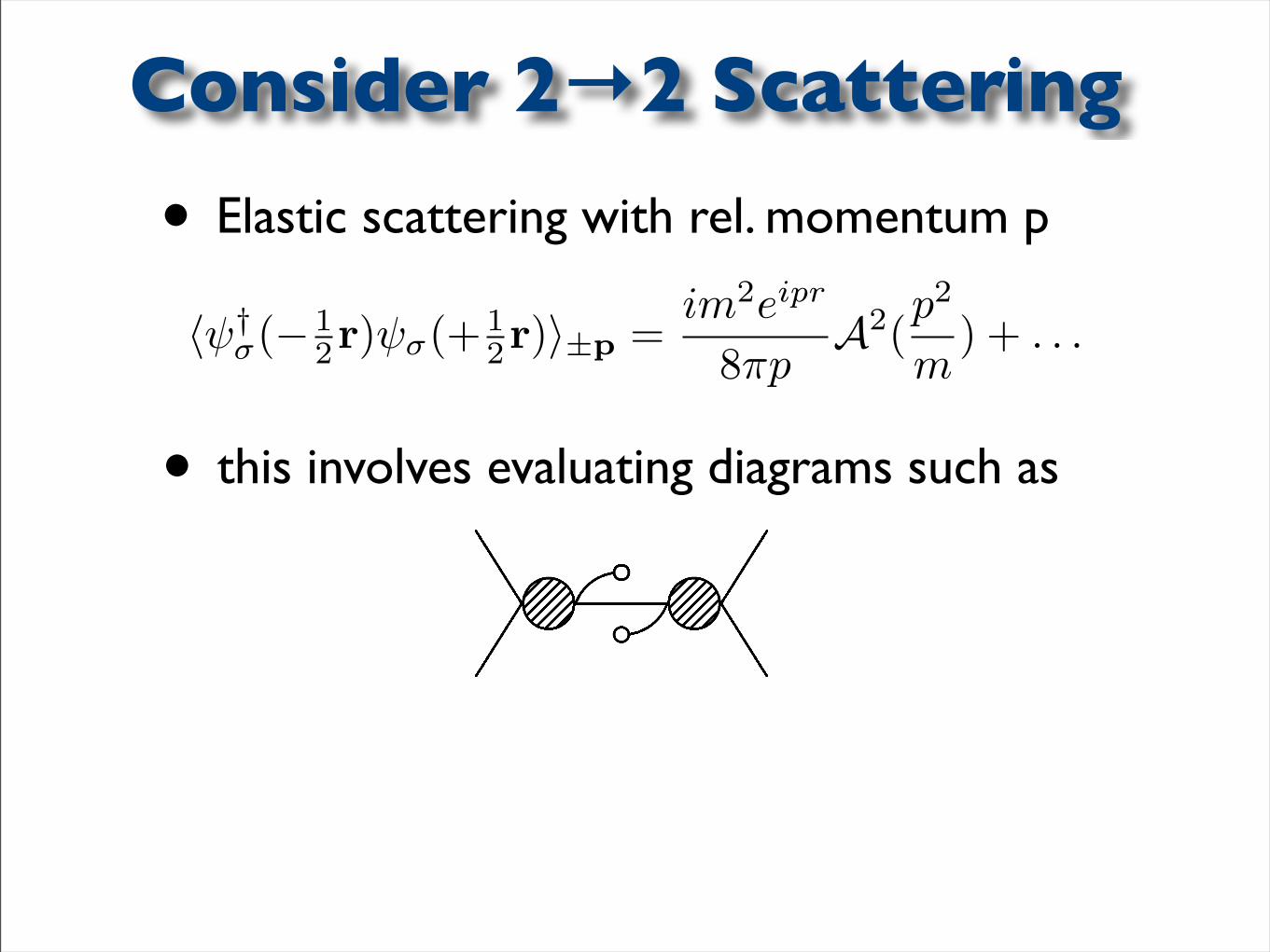
• Elastic scattering with rel. momentum p

Consider 2→2 Scattering

〈ψ†σ(− 12r)ψσ(+ 1

2r)〉±p =im2eipr

8πpA2(

p2

m) + . . .

• this involves evaluating diagrams such as

• Elastic scattering with rel. momentum p

Consider 2→2 Scattering

〈ψ†σ(− 12r)ψσ(+ 1

2r)〉±p =im2eipr

8πpA2(

p2

m) + . . .

• this involves evaluating diagrams such as

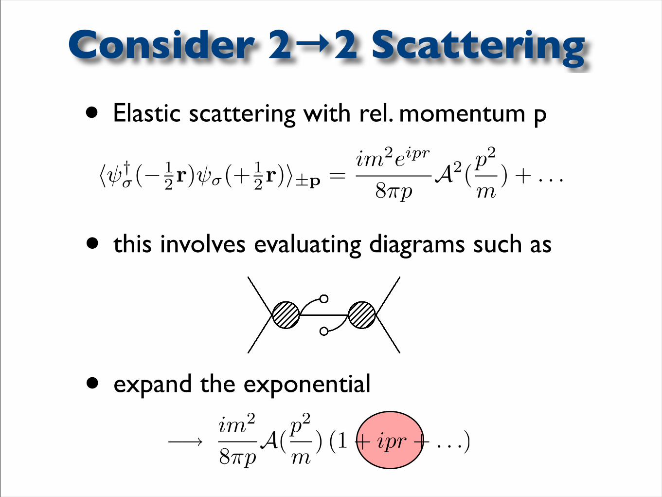
• expand the exponential

−→ im2

8πpA(

p2

m) (1 + ipr + . . .)

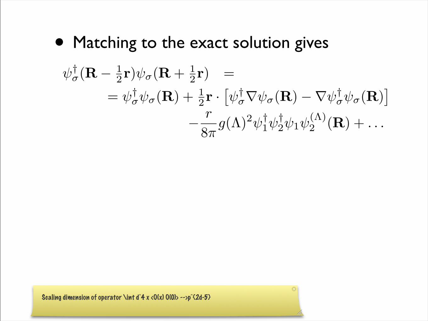
• Matching to the exact solution gives

ψ†σ(R− 1

2r)ψσ(R + 12r) =

= ψ†σψσ(R) + 1

2r ·[ψ†

σ∇ψσ(R)−∇ψ†σψσ(R)

]

− r

8πg(Λ)2ψ†

1ψ†2ψ1ψ

(Λ)2 (R) + . . .

Scaling dimension of operator \int d^4 x <O(x) O(0)> -->p^2d-5

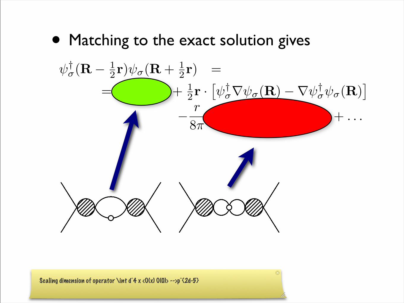
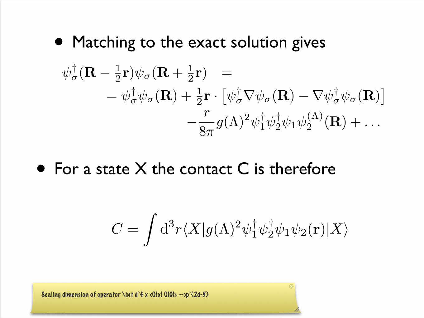
• Matching to the exact solution gives

ψ†σ(R− 1

2r)ψσ(R + 12r) =

= ψ†σψσ(R) + 1

2r ·[ψ†

σ∇ψσ(R)−∇ψ†σψσ(R)

]

− r

8πg(Λ)2ψ†

1ψ†2ψ1ψ

(Λ)2 (R) + . . .

Scaling dimension of operator \int d^4 x <O(x) O(0)> -->p^2d-5

• Matching to the exact solution gives

ψ†σ(R− 1

2r)ψσ(R + 12r) =

= ψ†σψσ(R) + 1

2r ·[ψ†

σ∇ψσ(R)−∇ψ†σψσ(R)

]

− r

8πg(Λ)2ψ†

1ψ†2ψ1ψ

(Λ)2 (R) + . . .

• For a state X the contact C is therefore

C =∫

d3r〈X|g(Λ)2ψ†1ψ

†2ψ1ψ2(r)|X〉

Scaling dimension of operator \int d^4 x <O(x) O(0)> -->p^2d-5

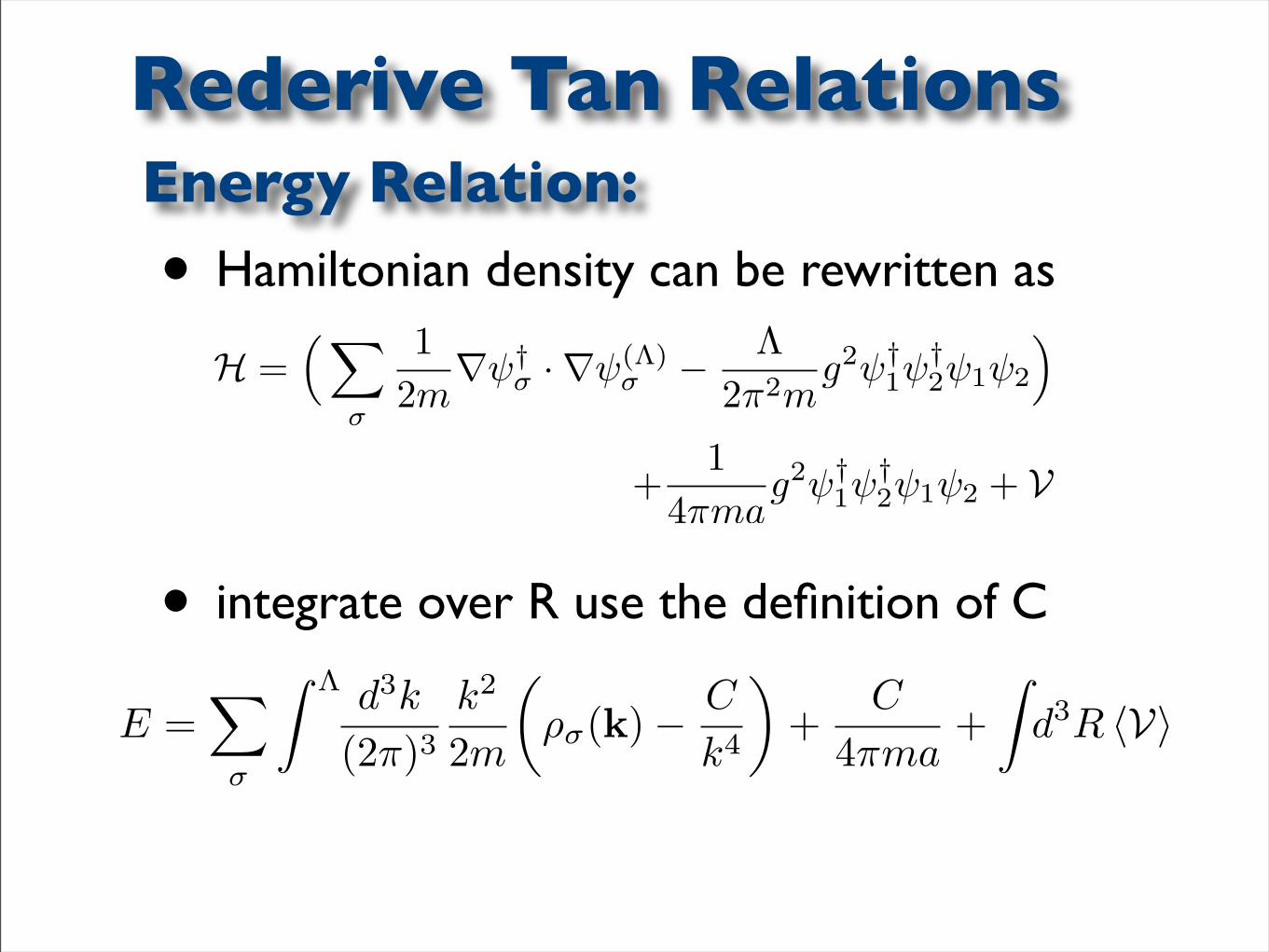
• Hamiltonian density can be rewritten as

• integrate over R use the definition of C

Rederive Tan RelationsEnergy Relation:

H =( ∑

σ

12m∇ψ†

σ ·∇ψ(Λ)σ − Λ

2π2mg2ψ†

1ψ†2ψ1ψ2

)

+1

4πmag2ψ†

1ψ†2ψ1ψ2 + V

E =∑

σ

∫ Λ d3k

(2π)3k2

2m

(ρσ(k) − C

k4

)+

C

4πma+

∫d3R 〈V〉

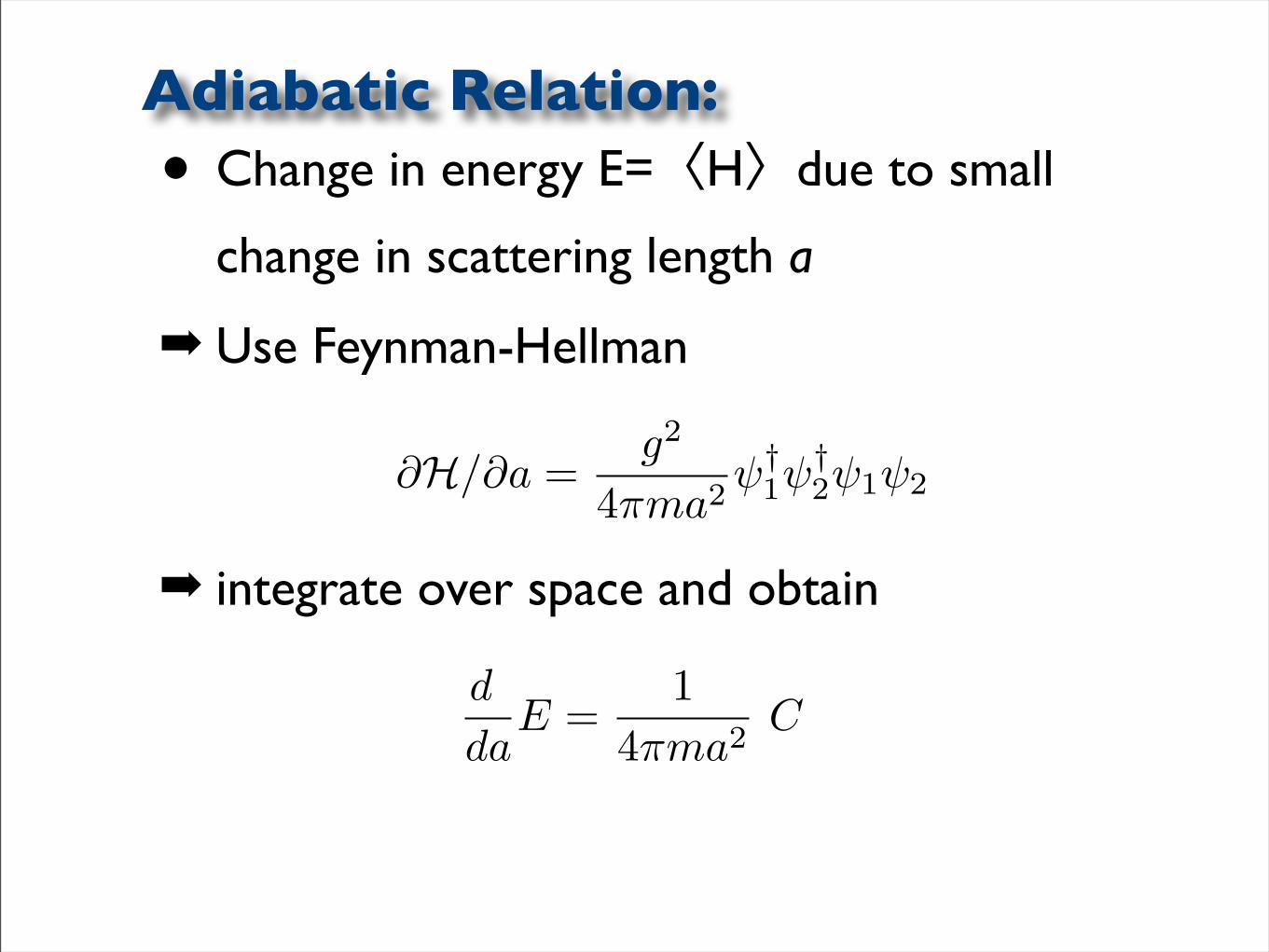
• Change in energy E=〈H〉due to small

change in scattering length a

Use Feynman-Hellman

integrate over space and obtain

Adiabatic Relation:

∂H/∂a =g2

4πma2ψ†

1ψ†2ψ1ψ2

d

daE =

14πma2

C

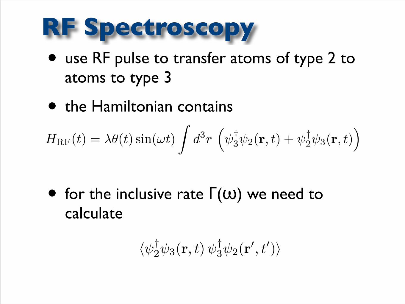
• use RF pulse to transfer atoms of type 2 to atoms to type 3

• the Hamiltonian contains

• for the inclusive rate Γ(ω) we need to calculate

RF Spectroscopy

HRF(t) = λθ(t) sin(ωt)∫

d3r(ψ†

3ψ2(r, t) + ψ†2ψ3(r, t)

)

〈ψ†2ψ3(r, t)ψ†

3ψ2(r′, t′)〉

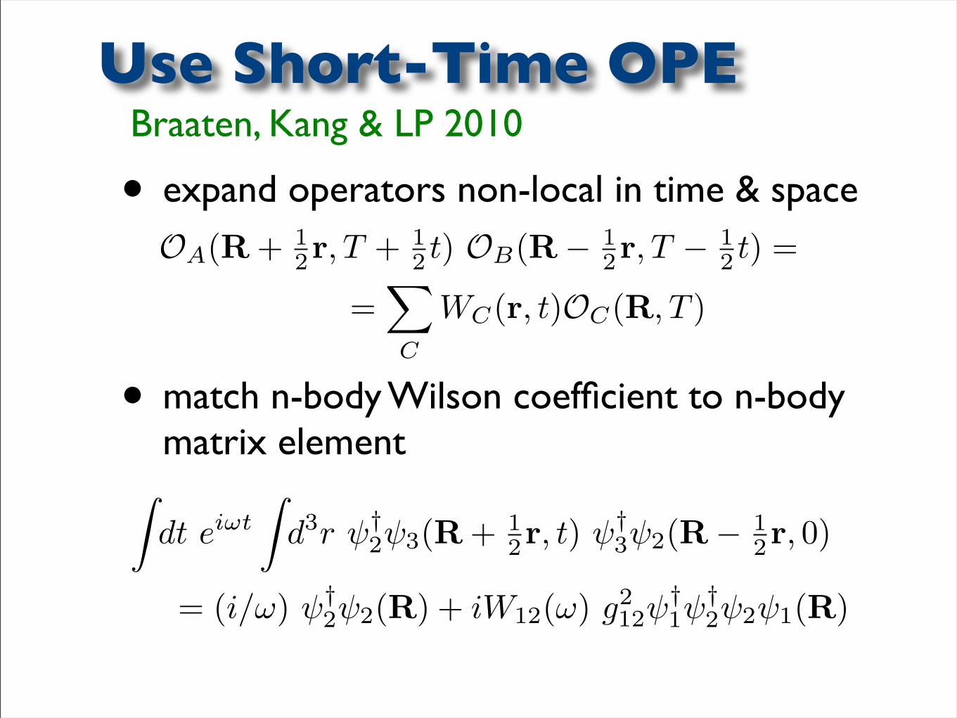
• expand operators non-local in time & space

• match n-body Wilson coefficient to n-body matrix element

Use Short-Time OPE

OA(R + 12r, T + 1

2 t) OB(R− 12r, T −

12 t) =

=∑

C

WC(r, t)OC(R, T )

Braaten, Kang & LP 2010

∫dt eiωt

∫d3r ψ†

2ψ3(R + 12r, t) ψ†

3ψ2(R− 12r, 0)

= (i/ω) ψ†2ψ2(R) + iW12(ω) g2

12ψ†1ψ

†2ψ2ψ1(R)

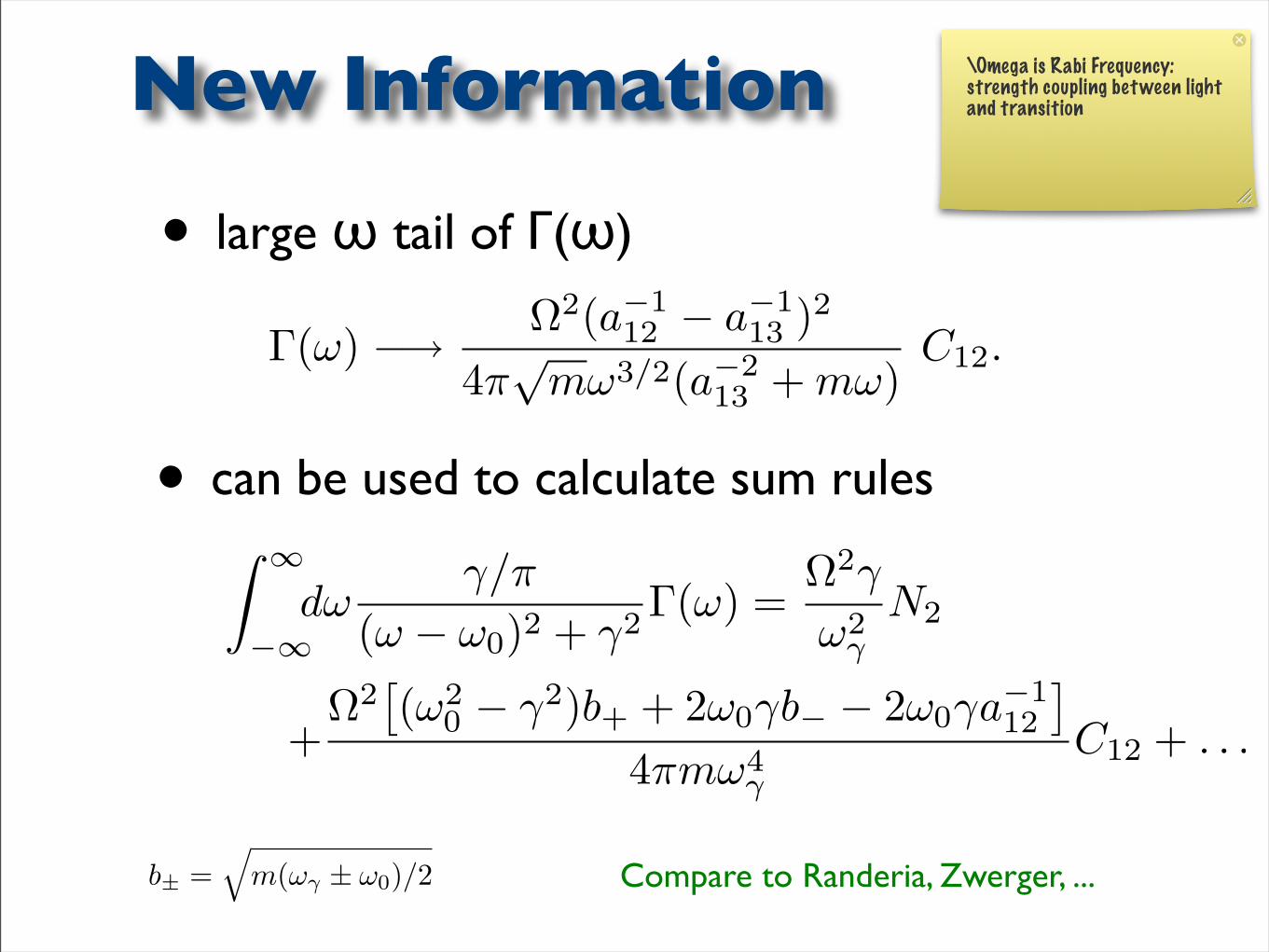
• large ω tail of Γ(ω)

New Information

Γ(ω) −→ Ω2(a−112 − a−1

13 )2

4π√

mω3/2(a−213 + mω)

C12.

• can be used to calculate sum rules

b± =√

m(ωγ ± ω0)/2

\Omega is Rabi Frequency: strength coupling between light and transition

Compare to Randeria, Zwerger, ...

∫ ∞

−∞dω

γ/π

(ω − ω0)2 + γ2Γ(ω) =

Ω2γ

ω2γ

N2

+Ω2

[(ω2

0 − γ2)b+ + 2ω0γb− − 2ω0γa−112

]

4πmω4γ

C12 + . . .

• Punk & Zwerger 2008

• Schneider & Randeria 2010

• Werner & Castin 2010

• Son & Thompson 2010

Active field of research

Theoretical:

Experimental:

• Hu et al. 2010

• Gaebler, Stewart & Jin 2010

• in few-body systems we can do calculations exactly

• what are the implications of a large scattering length in such systems

• what types of universality exist here

Let’s switch gears

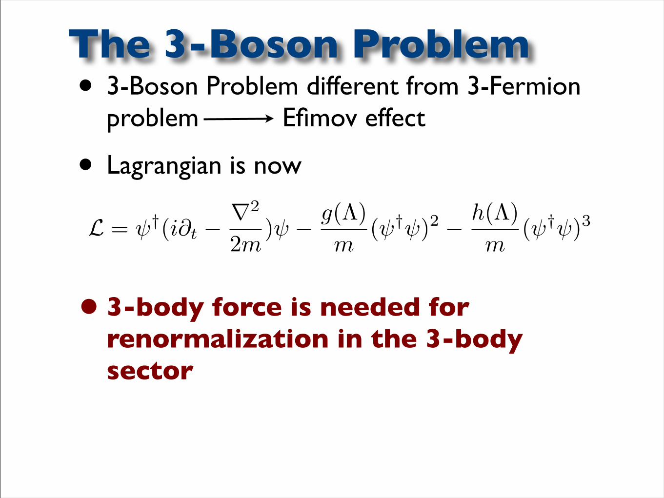
• 3-Boson Problem different from 3-Fermion problem Efimov effect

• Lagrangian is now

• 3-body force is needed for renormalization in the 3-body sector

The 3-Boson Problem

L = ψ†(i∂t −∇2

2m)ψ − g(Λ)

m(ψ†ψ)2 − h(Λ)

m(ψ†ψ)3

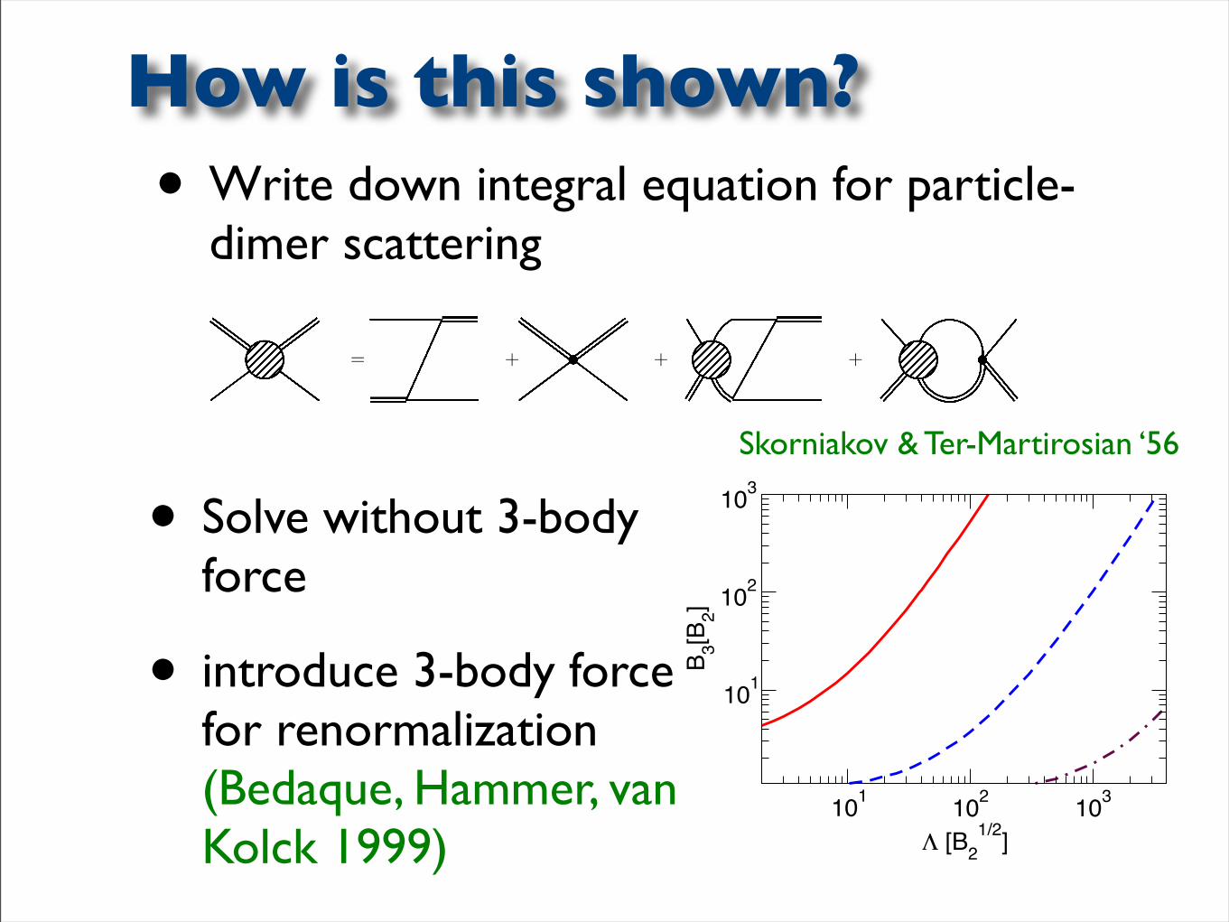
• Write down integral equation for particle-dimer scattering

How is this shown?

= + + +

• Solve without 3-body force

101 102 103

Λ [B21/2]

101

102

103

B 3[B2]

Skorniakov & Ter-Martirosian ‘56

• introduce 3-body force for renormalization (Bedaque, Hammer, van Kolck 1999)

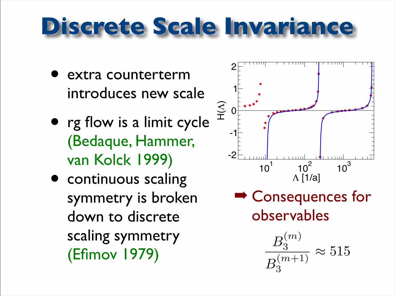
• extra counterterm introduces new scale

• rg flow is a limit cycle (Bedaque, Hammer, van Kolck 1999)

• continuous scaling symmetry is broken down to discrete scaling symmetry (Efimov 1979)

Discrete Scale Invariance

101 102 103

Λ [1/a]

-2

-1

0

1

2

H(Λ

)

Consequences for observables

B(m)3

B(m+1)3

≈ 515

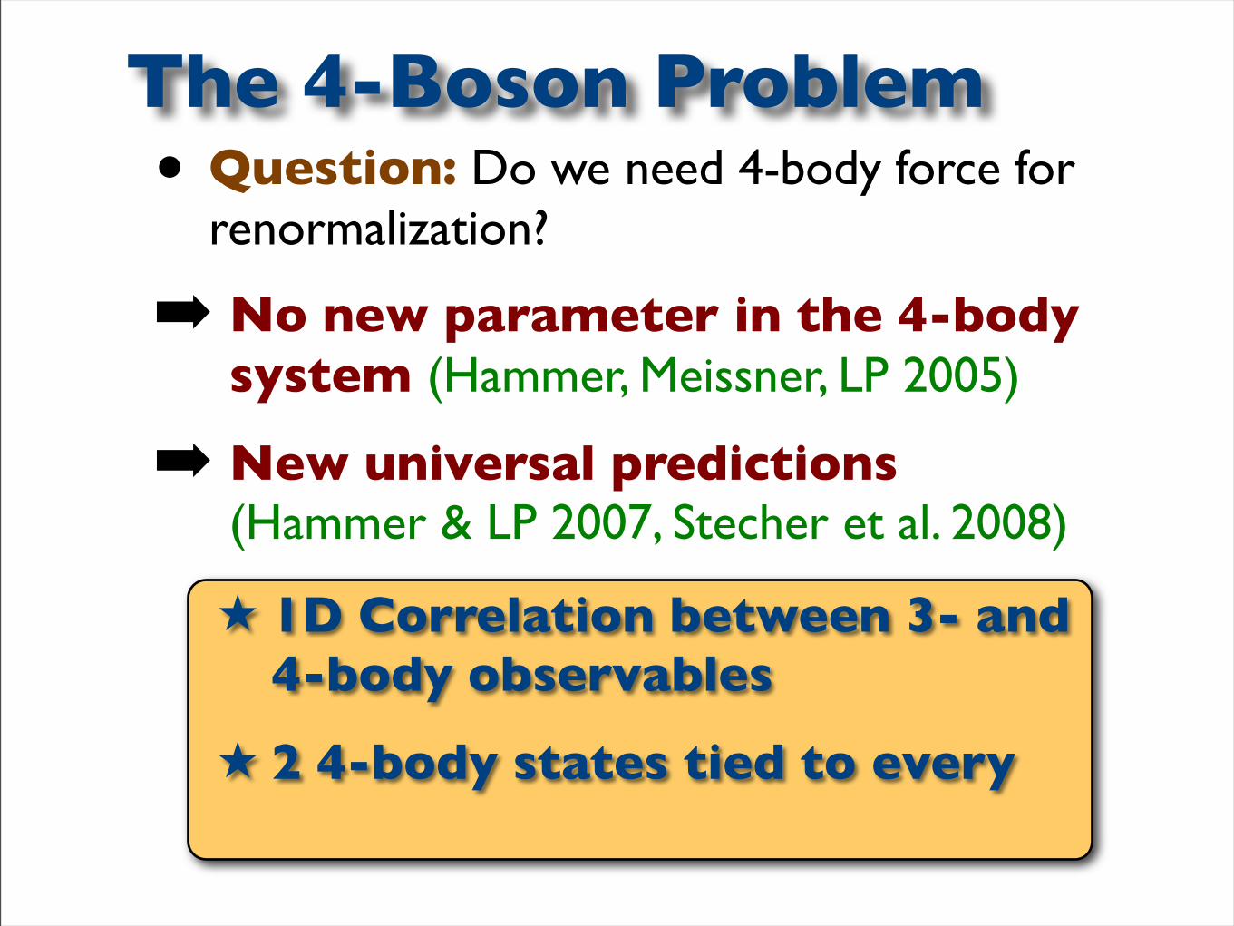
• Question: Do we need 4-body force for renormalization?

No new parameter in the 4-body system (Hammer, Meissner, LP 2005)

New universal predictions (Hammer & LP 2007, Stecher et al. 2008)

The 4-Boson Problem

1D Correlation between 3- and 4-body observables

2 4-body states tied to every

• Recombination features in AMO experiments display four-body features

Confirmed Experimentally

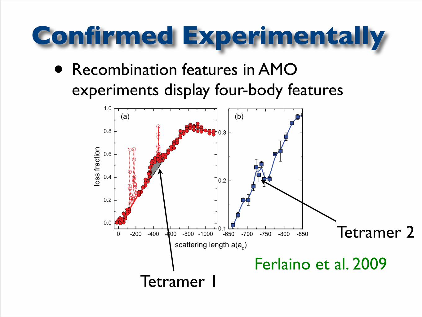
• Recombination features in AMO experiments display four-body features

Confirmed Experimentally

(a) (b)

Ferlaino et al. 2009Tetramer 1

Tetramer 2

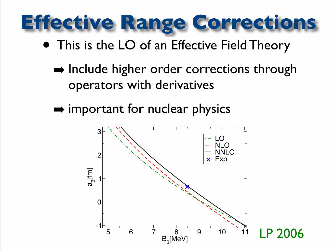
• This is the LO of an Effective Field Theory

Include higher order corrections through operators with derivatives

important for nuclear physics

Effective Range Corrections

5 6 7 8 9 10 11B3[MeV]

-1

0

1

2

3

a 3[fm

]

LONLONNLOExp

LP 2006

• Range corrections and power counting have been discussed mostly for fixed a

• Hammer & Mehen 2001

• Bedaque et al. 2003

• Phillips & LP 2006

• LP 2006

• What about variable scattering length?

Relevant for AMO and Lattice QCD exptrapolations

Range Corrections II

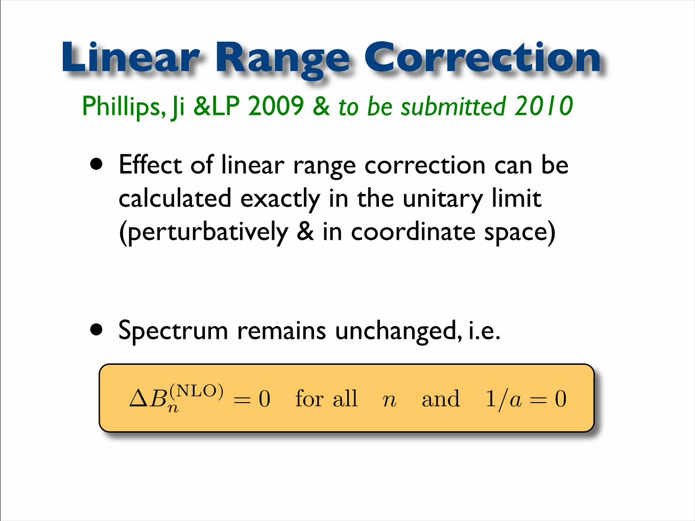
• Effect of linear range correction can be calculated exactly in the unitary limit (perturbatively & in coordinate space)

• Spectrum remains unchanged, i.e.

Linear Range CorrectionPhillips, Ji &LP 2009 & to be submitted 2010

∆B(NLO)n = 0 for all n and 1/a = 0

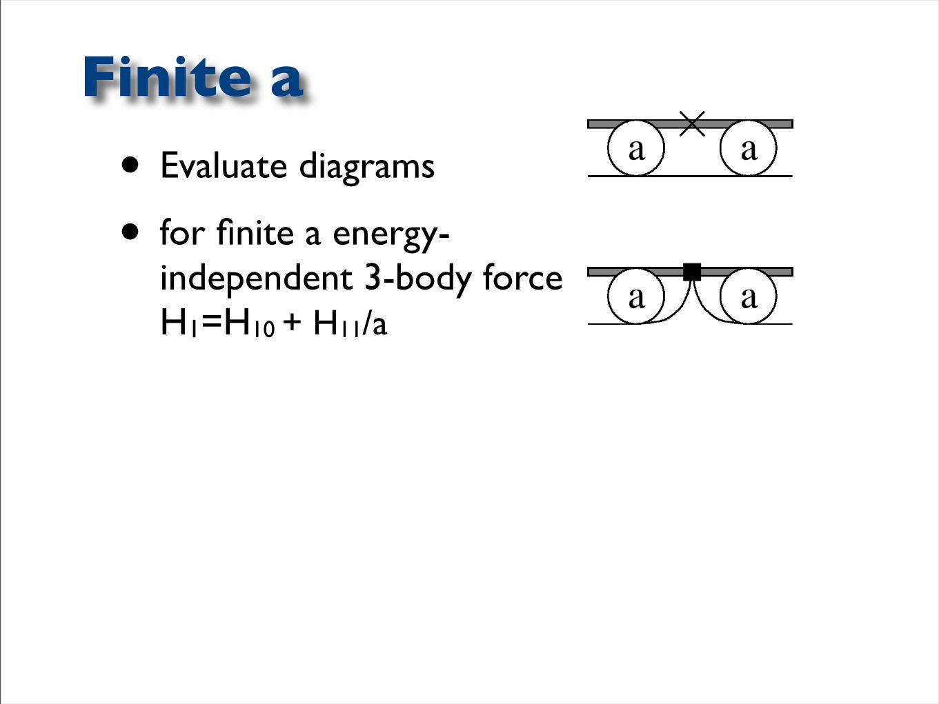
• Evaluate diagrams

• for finite a energy-independent 3-body force H1=H10 + H11/a

Finite a

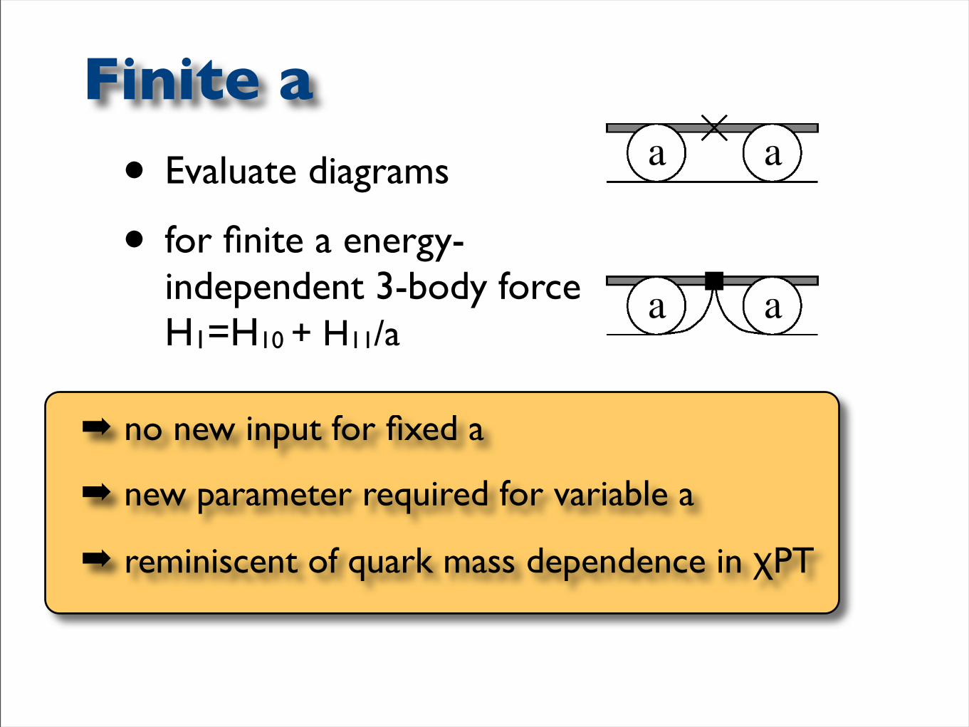
• Evaluate diagrams

• for finite a energy-independent 3-body force H1=H10 + H11/a

Finite a

no new input for fixed a

new parameter required for variable a

reminiscent of quark mass dependence in χPT

• Universality is important:

exact results for many-body systems

low-energy theorems for few-body systems

• Range corrections are important

first understand the physics then do the calculation

Summary