Neutron Rietveld RefinementR.B. Von DreeleAPS/IPNSArgonne National LaboratoryArgonne, Il 60439vondreele@anl.gov

“Rietveld refinement is one of those few fields of intellectual endeavor wherein the more one does it, the less one understands.” (Sue Kesson)

2

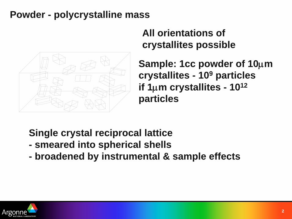
Powder - polycrystalline mass

All orientations of crystallites possible

Sample: 1cc powder of 10μm crystallites - 109 particlesif 1μm crystallites - 1012

particles

Single crystal reciprocal lattice - smeared into spherical shells- broadened by instrumental & sample effects

3

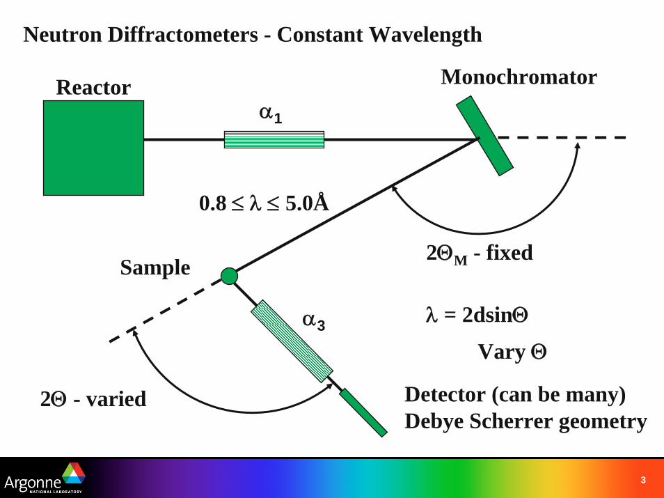
Neutron Diffractometers - Constant Wavelength

Reactor

Sample

α1

Detector (can be many)Debye Scherrer geometry

Monochromator

2ΘM - fixed

2Θ - varied

α3

0.8 ≤ λ ≤ 5.0Å

λ = 2dsinΘ

Vary Θ

4

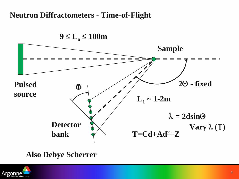
Neutron Diffractometers - Time-of-Flight

Sample

Detectorbank

L1 ~ 1-2m

Pulsedsource

9 ≤ Lo ≤ 100m

2Θ - fixed

λ = 2dsinΘVary λ (Τ)

Φ

Also Debye Scherrer

T=Cd+Ad2+Z

5

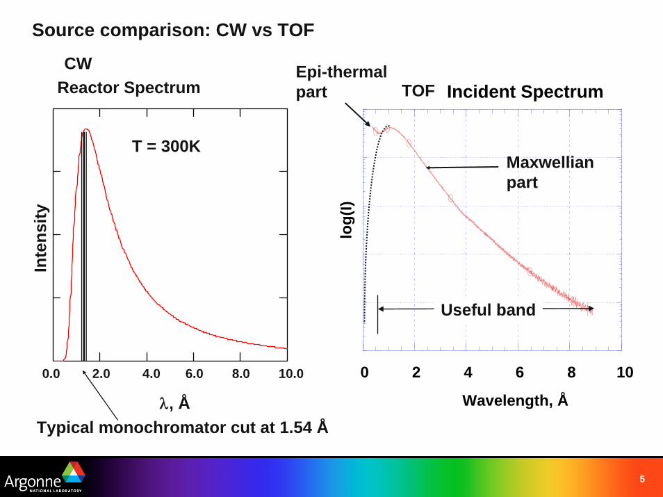
Reactor Spectrum

Inte

nsity

0.0 2.0 4.0 6.0 8.0 10.0

λ, ÅTypical monochromator cut at 1.54 Å

T = 300K

0 2 4 6 8 10

Incident Spectrum

log(

I)

Wavelength, Å

Maxwellianpart

Epi-thermalpart

Useful band

TOFCW

Source comparison: CW vs TOF

6

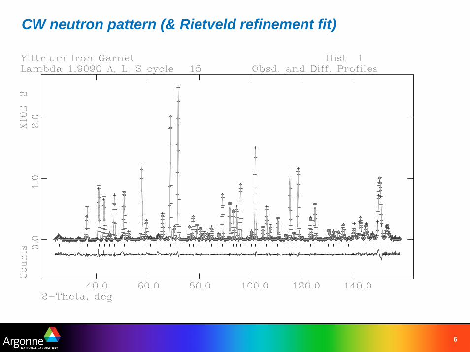
CW neutron pattern (& Rietveld refinement fit)

7

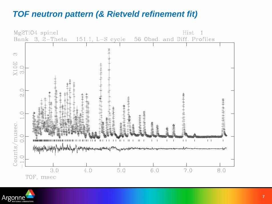
TOF neutron pattern (& Rietveld refinement fit)

8

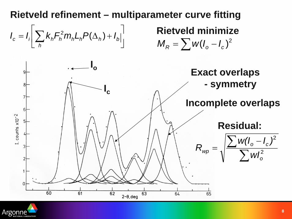
Rietveld refinement – multiparameter curve fitting

Exact overlaps - symmetry

Incomplete overlaps

Io

∑∑ −

= 2

2

o

cowp wI

)Iw(IR

Residual:

Rietveld minimize ∑ −= 2)( coR IIwM

Ic

⎥⎦

⎤⎢⎣

⎡+Δ= ∑

hbhhhhhic IPLmFkII )(2

9

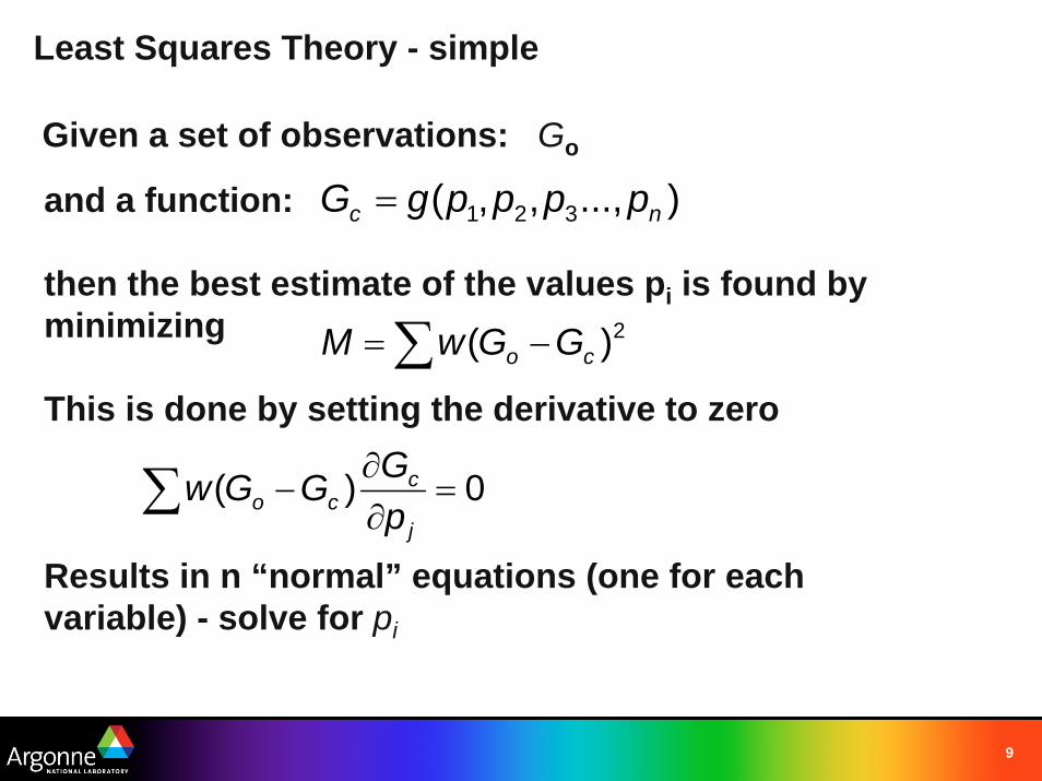
Least Squares Theory - simple

and a function:

then the best estimate of the values pi is found by minimizing

This is done by setting the derivative to zero

Results in n “normal” equations (one for each variable) - solve for pi

)...,,,( 321 nc ppppgG =

Given a set of observations: Go

2)( co GGwM −= ∑

0)( =∂∂

−∑j

cco p

GGGw

10

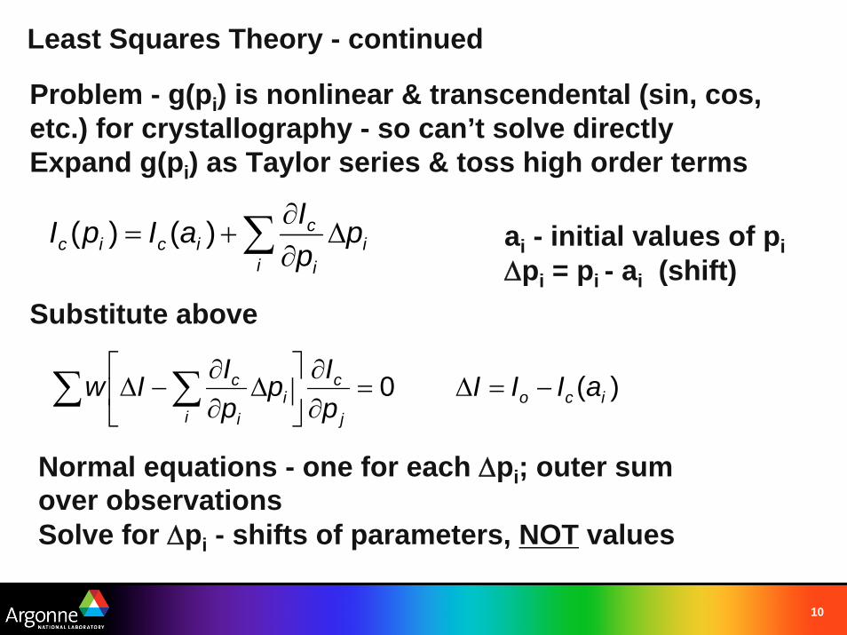
Least Squares Theory - continued

Problem - g(pi) is nonlinear & transcendental (sin, cos, etc.) for crystallography - so can’t solve directlyExpand g(pi) as Taylor series & toss high order terms

∑ Δ∂∂

+=i

ii

cicic p

pIaIpI )()(

Substitute above

ai - initial values of piΔpi = pi - ai (shift)

)(0 icoj

c

ii

i

c aIIIpIp

pIIw −=Δ=

∂∂

⎥⎦

⎤⎢⎣

⎡Δ

∂∂

−Δ∑ ∑

Normal equations - one for each Δpi; outer sum over observationsSolve for Δpi - shifts of parameters, NOT values

11

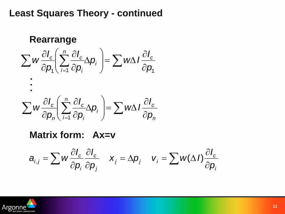
Least Squares Theory - continued

Rearrange

111 pIIwp

pI

pIw c

i

n

i i

cc

∂∂

Δ=⎟⎟⎠

⎞⎜⎜⎝

⎛Δ

∂∂

∂∂ ∑∑∑

=...

n

ci

n

i i

c

n

c

pIIwp

pI

pIw

∂∂

Δ=⎟⎟⎠

⎞⎜⎜⎝

⎛Δ

∂∂

∂∂ ∑∑∑

=1

Matrix form: Ax=v

i

cijj

j

c

i

cji p

IIwvpxpI

pIwa

∂∂

Δ=Δ=∂∂

∂∂

= ∑∑ )(,

12

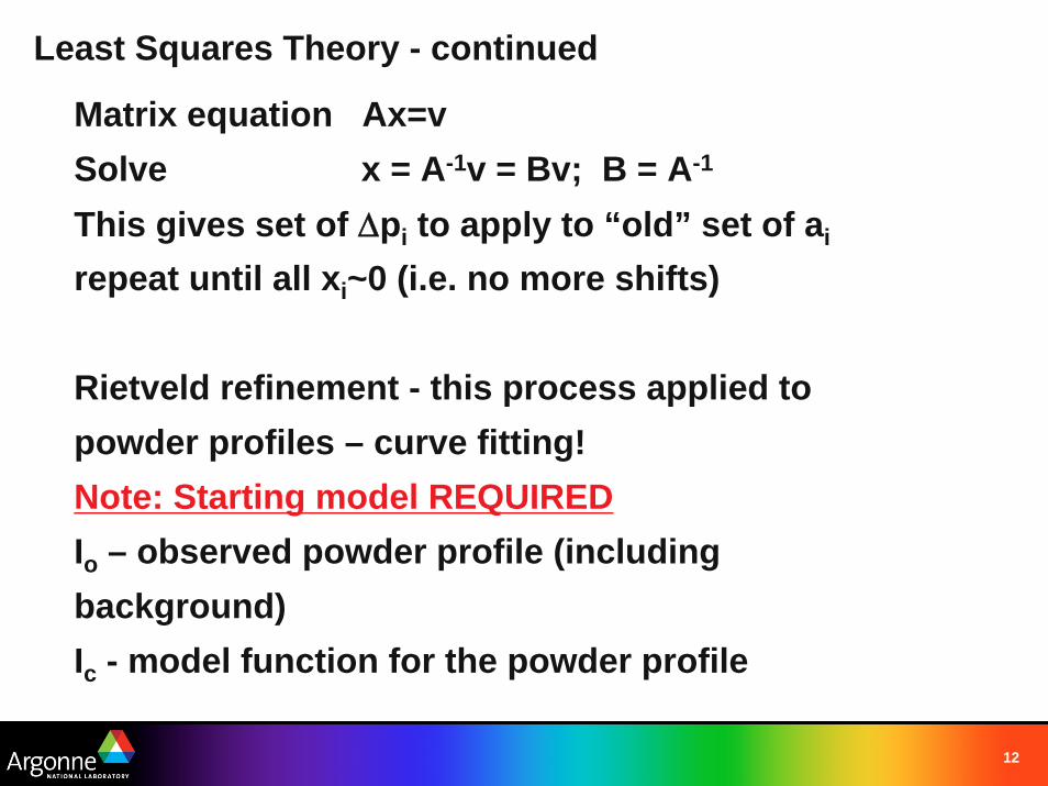
Least Squares Theory - continued

Matrix equation Ax=vSolve x = A-1v = Bv; B = A-1

This gives set of Δpi to apply to “old” set of ai

repeat until all xi~0 (i.e. no more shifts)

Rietveld refinement - this process applied to powder profiles – curve fitting!Note: Starting model REQUIREDIo – observed powder profile (including background)Ic - model function for the powder profile

13

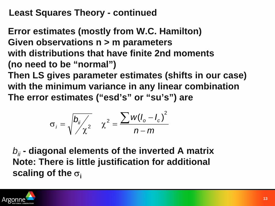
Least Squares Theory - continued

Error estimates (mostly from W.C. Hamilton)Given observations n > m parameterswith distributions that have finite 2nd moments (no need to be “normal”)Then LS gives parameter estimates (shifts in our case) with the minimum variance in any linear combinationThe error estimates (“esd’s” or “su’s”) are

mnIIwb coii

i −−

=χχ

=σ ∑ 22

2)(

bii - diagonal elements of the inverted A matrixNote: There is little justification for additional scaling of the σi

14

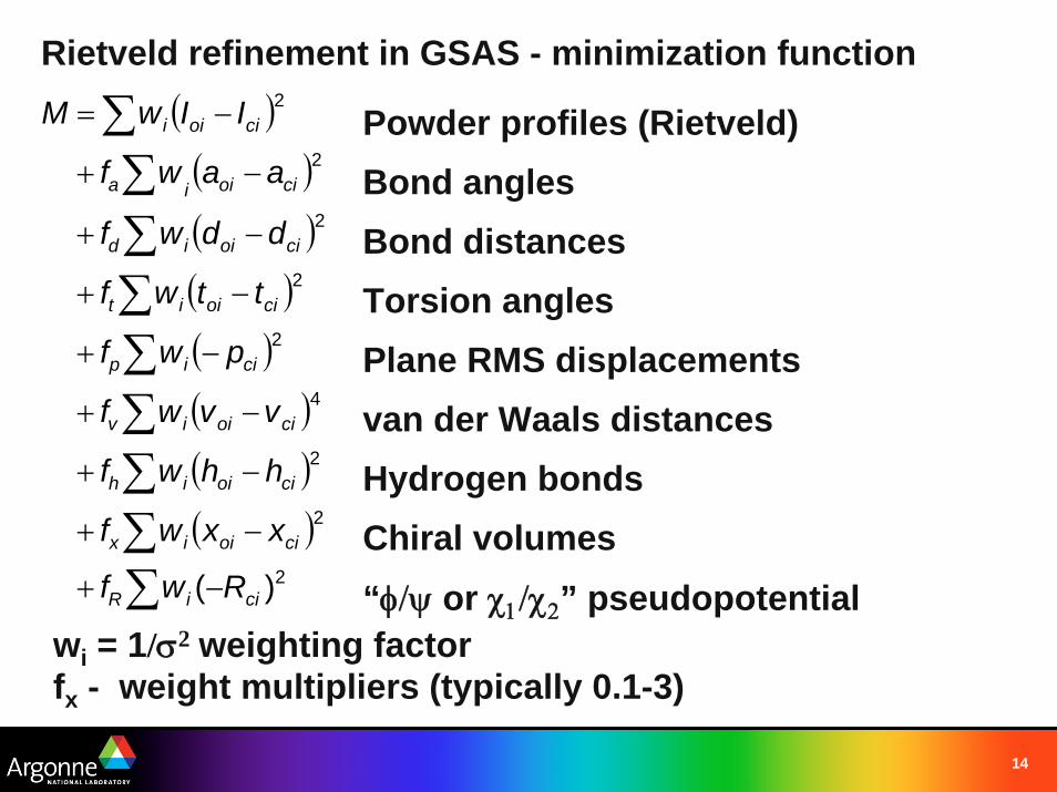
Rietveld refinement in GSAS - minimization function ( )

( )( )( )( )( )( )( )

2

2

2

4

2

2

2

2

2

)( ciiR

cioiix

cioiih

cioiiv

ciip

cioiit

cioiid

cioiia

cioii

Rwf

xxwf

hhwf

vvwf

pwf

ttwf

ddwf

aawf

IIwM

−+

−+

−+

−+

−+

−+

−+

−+

−=

∑∑∑∑∑∑∑∑

∑ Powder profiles (Rietveld)Bond anglesBond distancesTorsion anglesPlane RMS displacementsvan der Waals distancesHydrogen bondsChiral volumes“φ/ψ or χ1/χ2” pseudopotential

wi = 1/σ2 weighting factorfx - weight multipliers (typically 0.1-3)

15

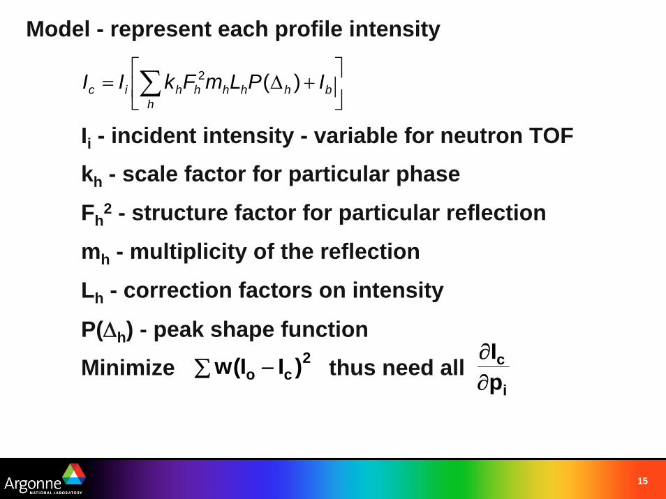
Model - represent each profile intensity

Ii - incident intensity - variable for neutron TOFkh - scale factor for particular phase

Fh2 - structure factor for particular reflection

mh - multiplicity of the reflection

Lh - correction factors on intensity

P(Δh) - peak shape functionMinimize thus need all

⎥⎦

⎤⎢⎣

⎡+Δ= ∑

hbhhhhhic IPLmFkII )(2

2co )II(w∑ −

i

cpI

∂∂

16

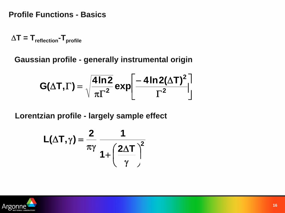
Profile Functions - Basics

Gaussian profile - generally instrumental origin

Lorentzian profile - largely sample effect

⎥⎦

⎤⎢⎣

⎡Γ

Δ−Γπ

=ΓΔ 2

2

2)T(2ln4exp2ln4),T(G

ΔT = Treflection-Tprofile

2T21

12),T(L⎟⎠⎞

⎜⎝⎛

γΔ+

πγ=γΔ

17

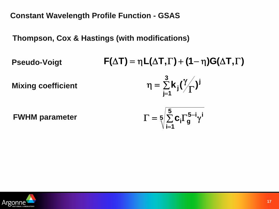
Constant Wavelength Profile Function - GSAS

Thompson, Cox & Hastings (with modifications)

Pseudo-Voigt ),T(G)1(),T(L)T(F ΓΔη−+ΓΔη=Δ

Mixing coefficient j3

1jj )(k∑ Γ

γ=η=

FWHM parameter 55

1i

ii5gic∑ γΓ=Γ

=

−

18

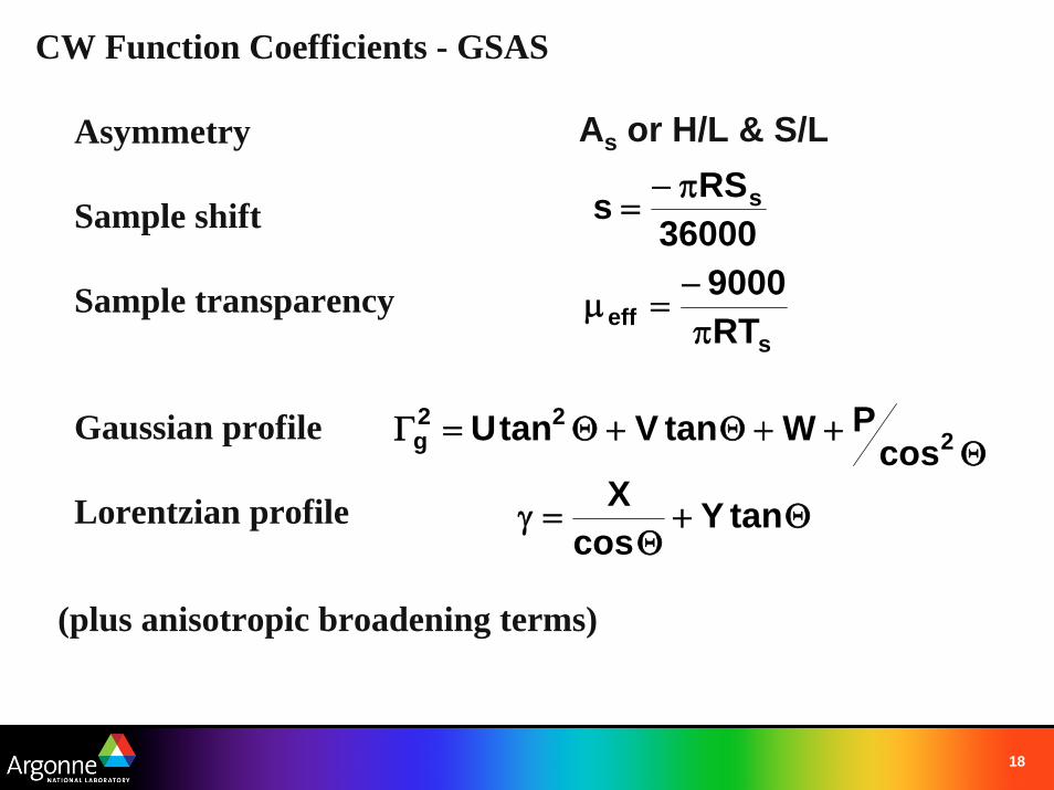
CW Function Coefficients - GSAS

Asymmetry

Sample shift

Sample transparency

Gaussian profile

Lorentzian profile

As or H/L & S/L

36000RSs sπ−

=

seff RT

9000π

−=μ

Θ++Θ+Θ=Γ 2

22g cos

PWtanVtanU

Θ+Θ

=γ tanYcos

X

(plus anisotropic broadening terms)

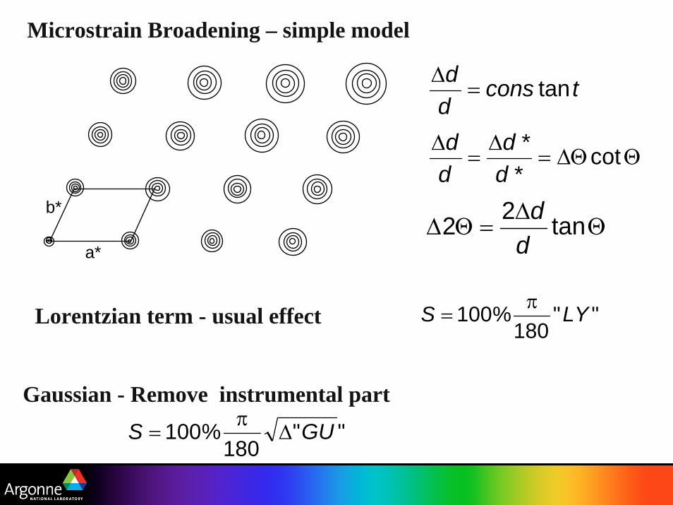
Microstrain Broadening – simple model

a*

b*

tconsdd tan=

Δ

ΘΔΘ=Δ

=Δ cot

**

dd

dd

ΘΔ

=ΘΔ tan22d

d

Lorentzian term - usual effect ""180

%100 LYS π=

Gaussian - Remove instrumental part

""180

%100 GUS Δπ

=

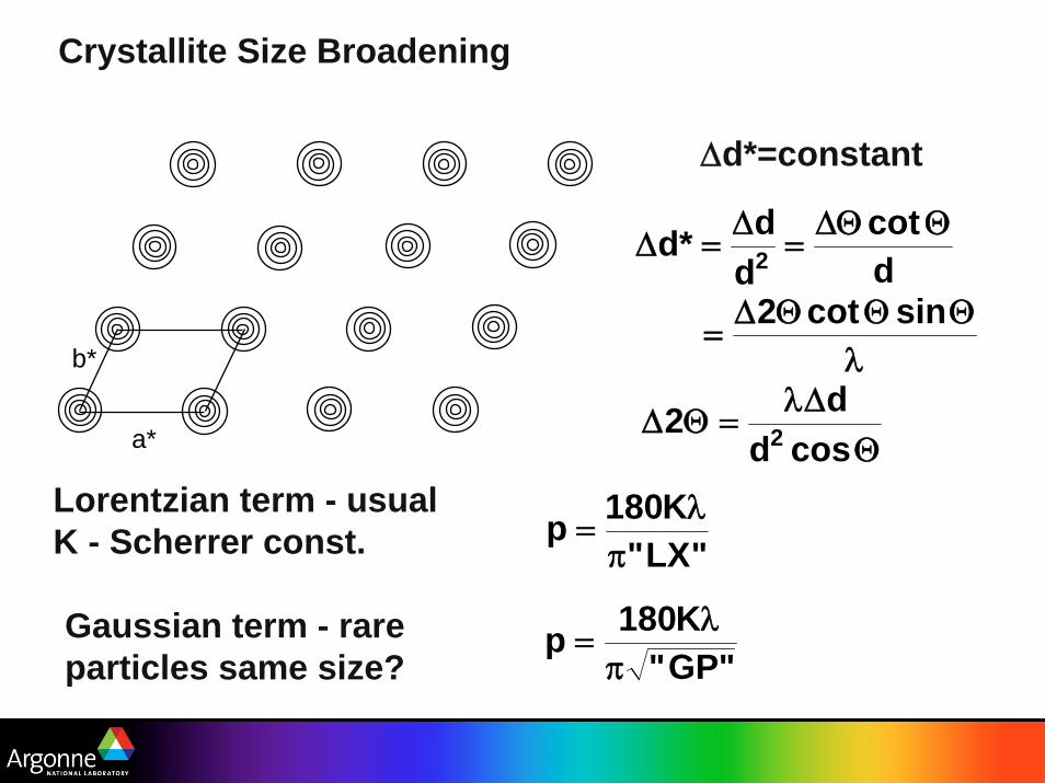
Crystallite Size Broadening

a*

b*

Δd*=constant

dcot

dd*d 2

ΘΔΘ=

Δ=Δ

λΘΘΘΔ

=sincot2

ΘΔλ

=ΘΔcosd

d2 2

Lorentzian term - usualK - Scherrer const. "LX"

K180pπ

λ=

Gaussian term - rareparticles same size? "GP"

K180pπ

λ=

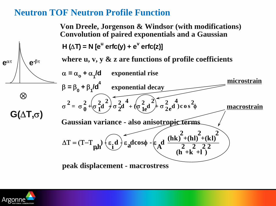
Neutron TOF Neutron Profile FunctionVon Dreele, Jorgenson & Windsor (with modifications)Convolution of paired exponentials and a Gaussian

where u, v, y & z are functions of profile coefficients

exponential rise

exponential decay

Gaussian variance - also anisotropic terms

H (ΔT) = N [eu erfc(y) + ev erfc(z)]

α = αo + α1/d

β = β0 + β1/d4

σ 2 = σ 02 + σ 1

2d2

+ σ 22d

4+ (σ 1e

2 d2

+ σ 2e2 d

4)c o s 2φ

peak displacement - macrostress

ΔΤ = (Τ−Τp,h) - εid - εadcosφ - εAd(h

2+k

2+l

2)2

(hk)2+(hl)

2+(kl)

2

microstrain

macrostrain

eατ e-βτ

⊗

G(ΔT,σ)

22

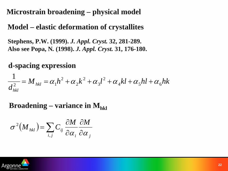
Microstrain broadening – physical model

Stephens, P.W. (1999). J. Appl. Cryst. 32, 281-289.Also see Popa, N. (1998). J. Appl. Cryst. 31, 176-180.

Model – elastic deformation of crystallites

hkhlkllkhMd hkl

hkl654

23

22

212

1 αααααα +++++==

d-spacing expression

( ) ∑ ∂∂

∂∂

=ji ji

ijhklMMCM

,

2

αασ

Broadening – variance in Mhkl

23

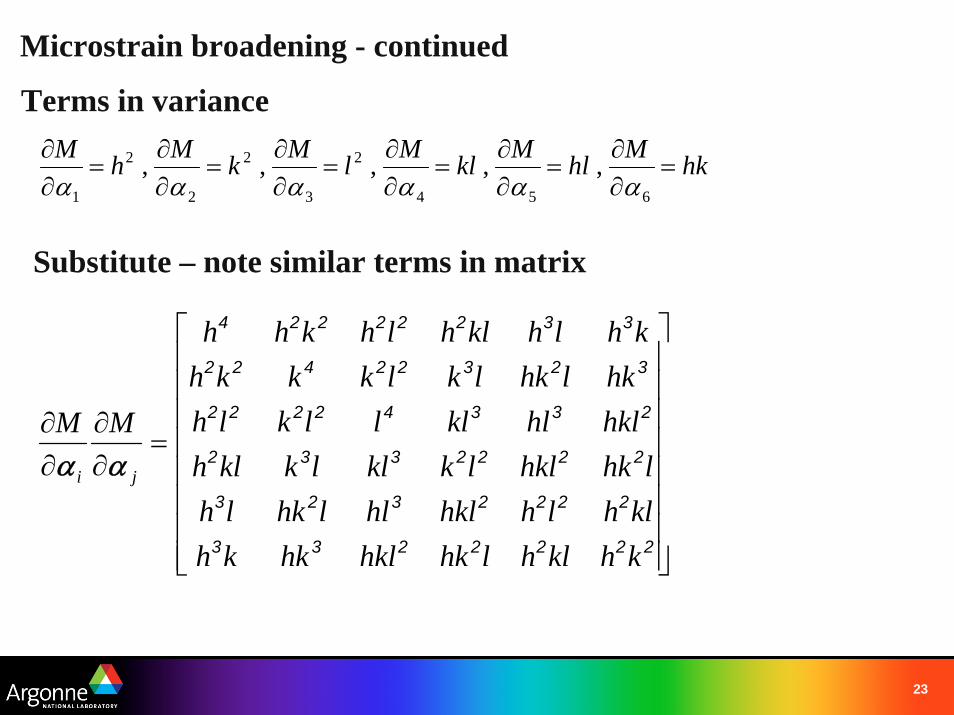
hkMhlMklMlMkMhM=

∂∂

=∂∂

=∂∂

=∂∂

=∂∂

=∂∂

654

2

3

2

2

2

1

,,,,,αααααα

⎥⎥⎥⎥⎥⎥⎥⎥

⎦

⎤

⎢⎢⎢⎢⎢⎢⎢⎢

⎣

⎡

=∂∂

∂∂

2222233

2222323

2222332

23342222

32322422

33222224

khklhlhkhklhkkhklhlhhklhllhklhlhkhkllkkllkklh

hklhlklllklhhklhklklkkkh

khlhklhlhkhh

MM

ji αα

Microstrain broadening - continued

Terms in variance

Substitute – note similar terms in matrix

24

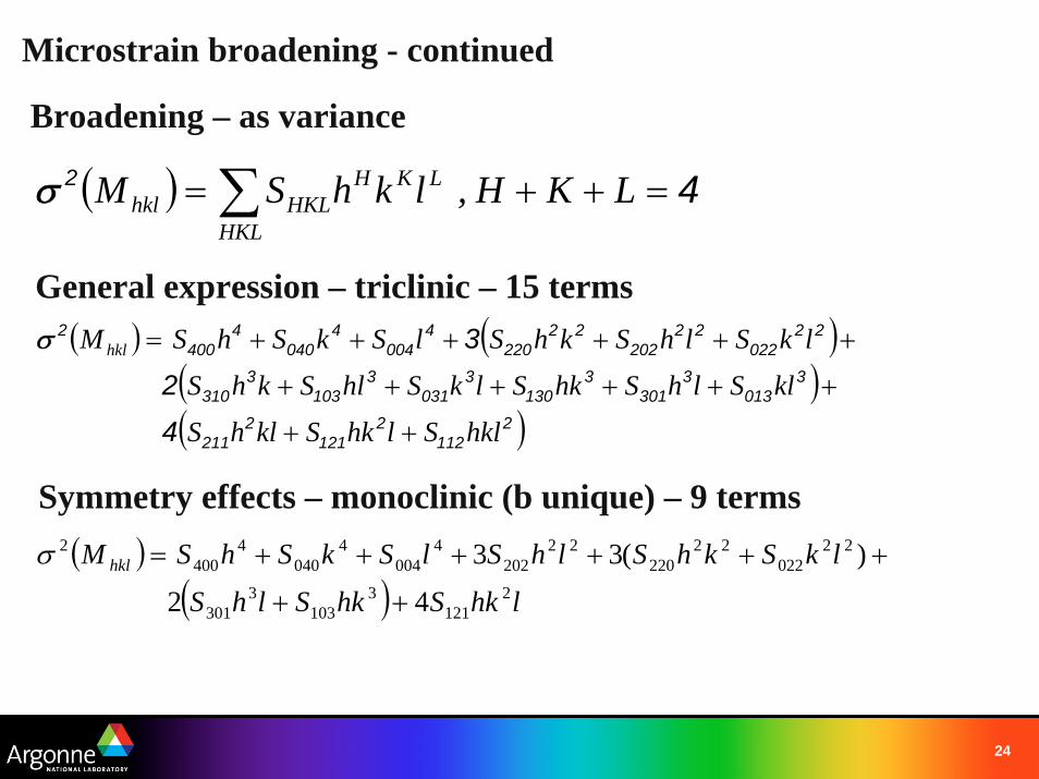
( ) 42 =++= ∑ LKH,lkhSMHKL

LKHHKLhklσ

( ) ( )( )( )2

1122

1212

211

3013

3301

3130

3031

3103

3310

22022

22202

22220

4004

4040

4400

2

42

3

hklSlhkSklhS

klSlhShkSlkShlSkhS

lkSlhSkhSlSkShSM hkl

++

++++++

++++++=σ

Microstrain broadening - continued

Broadening – as variance

General expression – triclinic – 15 terms

Symmetry effects – monoclinic (b unique) – 9 terms( )

( ) lhkShkSlhS

lkSkhSlhSlSkShSM hkl2

1213

1033

301

22022

22220

22202

4004

4040

4400

2

42

)(33

++

++++++=σ

25

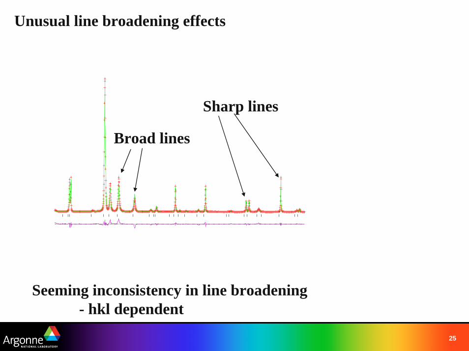
Na benzoate test Hist 1Lambda 1.1475 A, L-S cycle 167 Obsd. and Diff. Profiles

2-Theta, deg

Counts

X10E 1 2.0 2.1 2.2 2.3 2.4 2.5 2.6 2.7 2.8 2.9 3.0

X10E 4

.0

2.0

4.0

6.0

Unusual line broadening effects

Sharp lines

Broad lines

Seeming inconsistency in line broadening- hkl dependent

26

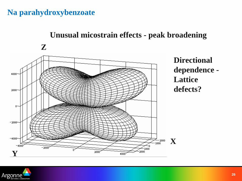
Na parahydroxybenzoate

Unusual micostrain effects - peak broadening

Directional dependence -Lattice defects?

XY

Z

27

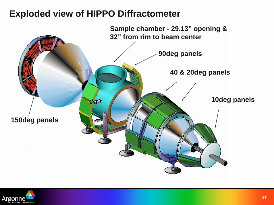
Exploded view of HIPPO DiffractometerSample chamber - 29.13” opening &32” from rim to beam center

150deg panels

10deg panels

40 & 20deg panels

90deg panels

28

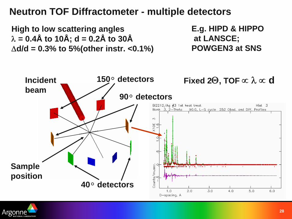
Neutron TOF Diffractometer - multiple detectors

Incident beam

150° detectors

90° detectors

40° detectors

Sample position

Fixed 2Θ, TOF ∝ λ ∝ d

E.g. HIPD & HIPPOat LANSCE;

POWGEN3 at SNS

High to low scattering anglesλ = 0.4Å to 10Å; d = 0.2Å to 30ÅΔd/d = 0.3% to 5%(other instr. <0.1%)

29

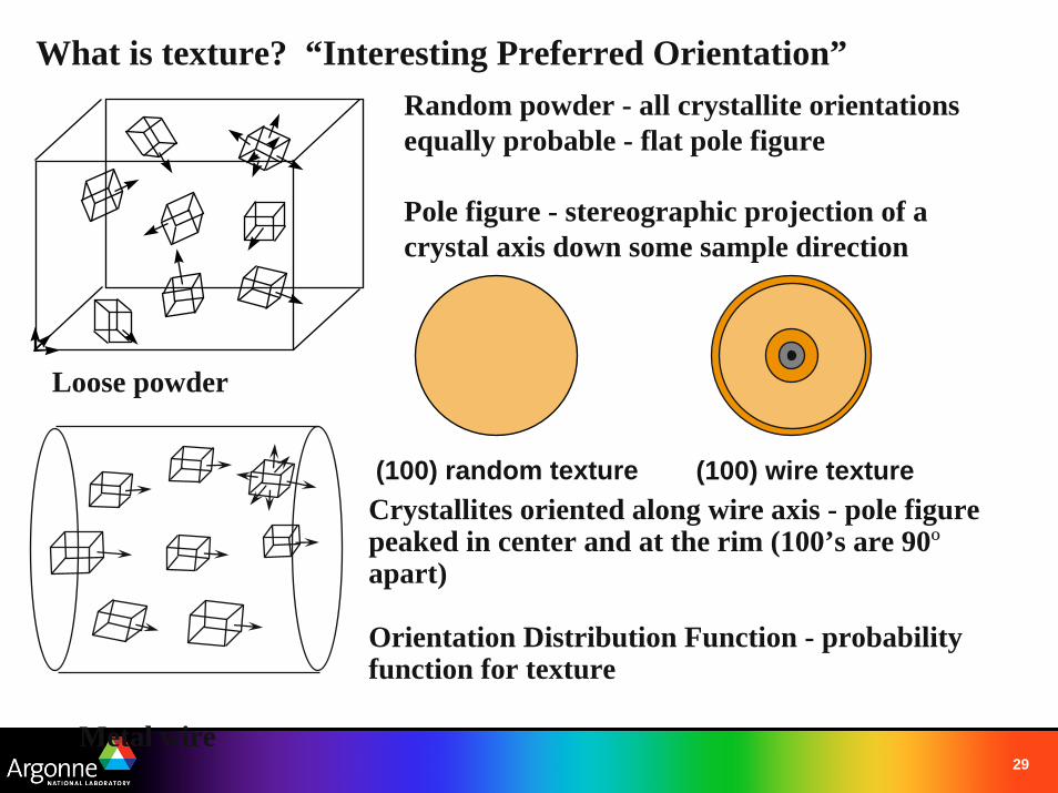
Random powder - all crystallite orientations equally probable - flat pole figure

Crystallites oriented along wire axis - pole figure peaked in center and at the rim (100’s are 90ºapart)

Orientation Distribution Function - probability function for texture

(100) wire texture(100) random texture

What is texture? “Interesting Preferred Orientation”

Pole figure - stereographic projection of a crystal axis down some sample direction

Loose powder

Metal wire

30

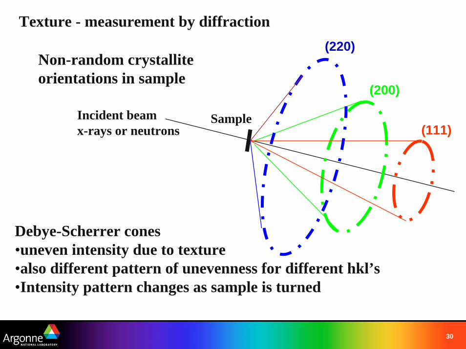
Texture - measurement by diffraction

Debye-Scherrer cones •uneven intensity due to texture •also different pattern of unevenness for different hkl’s•Intensity pattern changes as sample is turned

Non-random crystallite orientations in sample

Incident beamx-rays or neutrons

Sample(111)

(200)

(220)

31

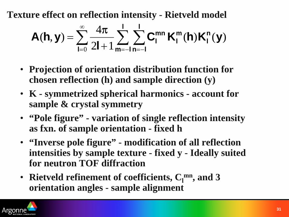
• Projection of orientation distribution function for chosen reflection (h) and sample direction (y)

• K - symmetrized spherical harmonics - account for sample & crystal symmetry

• “Pole figure” - variation of single reflection intensity as fxn. of sample orientation - fixed h

• “Inverse pole figure” - modification of all reflection intensities by sample texture - fixed y - Ideally suited for neutron TOF diffraction

• Rietveld refinement of coefficients, Clmn, and 3

orientation angles - sample alignment

Texture effect on reflection intensity - Rietveld model

)()(12

4),(0

yKhKCl

yhA nl

ml

l

lm

l

ln

mnl

l∑ ∑∑

−= −=

∞

= +=

π

32

, , y

D-spacing, A

Coun

ts/mu

sec.

1.0 2.0 3.0 4.0

X10E

2

-2.0

.0

2.

0

4.0

6.

0

y

D-spacing, A

Coun

ts/mu

sec.

1.0 2.0 3.0 4.0 5.0 6.0

X10E

3

.0

1.0

2.

0

3.0

4.

0

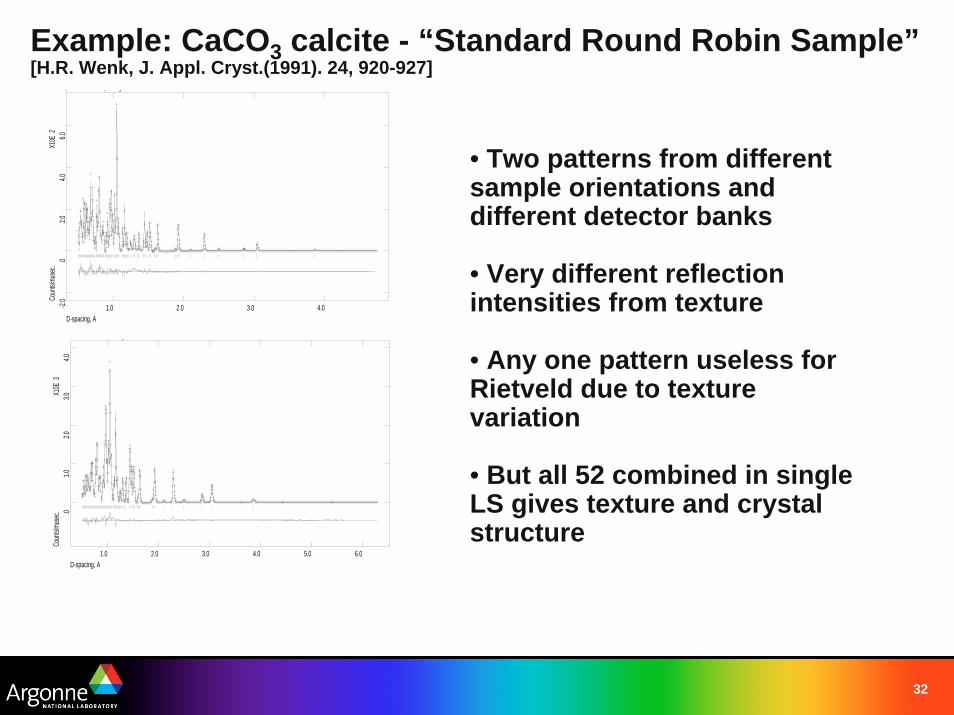
• Two patterns from different sample orientations and different detector banks

• Very different reflection intensities from texture

• Any one pattern useless for Rietveld due to texture variation

• But all 52 combined in single LS gives texture and crystal structure

Example: CaCO3 calcite - “Standard Round Robin Sample”[H.R. Wenk, J. Appl. Cryst.(1991). 24, 920-927]

33

calcite 0 0 6 Pole Figure - Equal Area

C

1

2

3

4

5

6

7

8

9

10

11

12 13 14

15

16

17

18

19

20

21

22

23

24 25 26

27 28

29

30

31

32

33

34

35

36

37 38

39

40

41

42

43

44

45

46

47

48

49 50

51

52

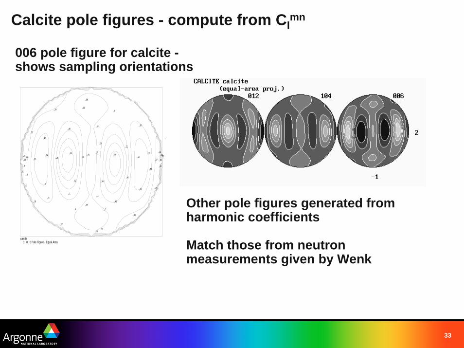
006 pole figure for calcite -shows sampling orientations

Other pole figures generated from harmonic coefficients

Match those from neutron measurements given by Wenk

Calcite pole figures - compute from Clmn

34

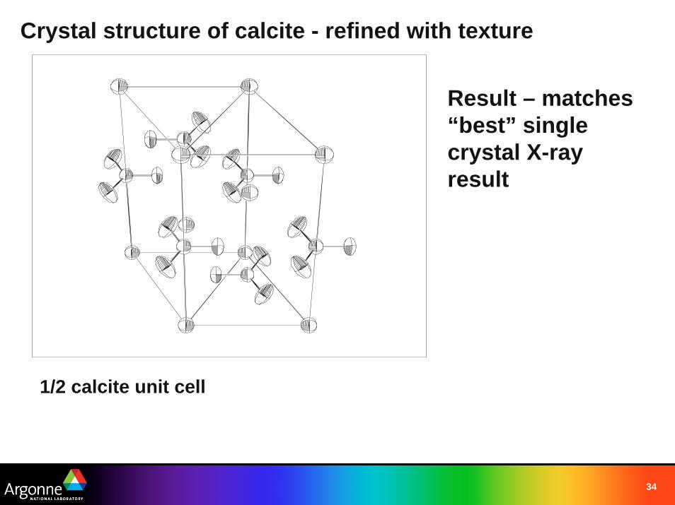
Crystal structure of calcite - refined with texture

1/2 calcite unit cell

Result – matches “best” single crystal X-ray result

35

A final word

“A Rietveld refinement is never perfected, merely abandoned”

(P. Stephens, 2000)