
Treatment of the Multiple Coulomb Scattering (MCS) · angle MCS in the mixed mode, is taken into...
11
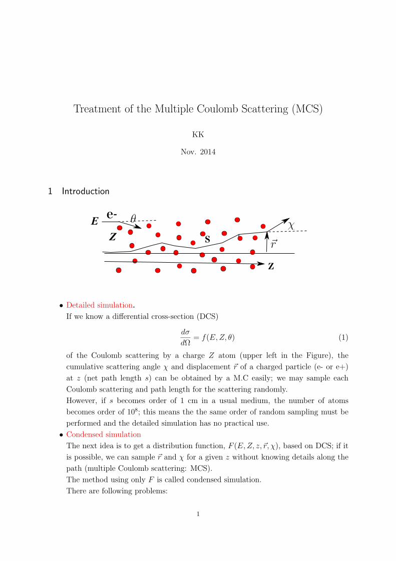
Treatment of the Multiple Coulomb Scattering (MCS) KK Nov. 2014 1 Introduction e- E Z θ χ r z s • Detailed simulation. If we know a differential cross-section (DCS) dσ dΩ = f (E,Z,θ) (1) of the Coulomb scattering by a charge Z atom (upper left in the Figure), the cumulative scattering angle χ and displacement r of a charged particle (e- or e+) at z (net path length s) can be obtained by a M.C easily; we may sample each Coulomb scattering and path length for the scattering randomly. However, if s becomes order of 1 cm in a usual medium, the number of atoms becomes order of 10 8 ; this means the the same order of random sampling must be performed and the detailed simulation has no practical use. • Condensed simulation The next idea is to get a distribution function, F (E,Z,z, r, χ), based on DCS; if it is possible, we can sample r and χ for a given z without knowing details along the path (multiple Coulomb scattering: MCS). The method using only F is called condensed simulation. There are following problems: 1
-
Upload
nguyenduong -
Category
Documents
-
view
213 -
download
0
Transcript of Treatment of the Multiple Coulomb Scattering (MCS) · angle MCS in the mixed mode, is taken into...
Treatment of the Multiple Coulomb Scattering (MCS)
KK
Nov. 2014
1 Introduction
e-EZ
r
z
s
• Detailed simulation.
If we know a differential cross-section (DCS)
dσ
dΩ= f(E,Z, θ) (1)
of the Coulomb scattering by a charge Z atom (upper left in the Figure), the
cumulative scattering angle χ and displacement r of a charged particle (e- or e+)
at z (net path length s) can be obtained by a M.C easily; we may sample each
Coulomb scattering and path length for the scattering randomly.
However, if s becomes order of 1 cm in a usual medium, the number of atoms
becomes order of 108; this means the the same order of random sampling must be
performed and the detailed simulation has no practical use.
• Condensed simulation
The next idea is to get a distribution function, F (E,Z, z, r, χ), based on DCS; if it
is possible, we can sample r and χ for a given z without knowing details along the
path (multiple Coulomb scattering: MCS).
The method using only F is called condensed simulation.
There are following problems:
1
– It’s not possible to solve the equation expressing F (diffusion equation).
– Fermi expressed F (r, χ) by a Gaussian distribution (the central limiting theorem
would imply it’s not so bad). It contains r, χ correlation.
It is not obvious how to determine the average and dispersion. Normally,
those given in PDB are used (In Epics, Moliere=0 corresponds to this. With
AlateCor=1 or 2, r correlated with χ is sampled. If AlateCor=0, only angle is
sampled.
– Goudsmit & Sandaerson obtained formal solution of F (χ) without assuming
DCS. But for a given realistic DCS, computation is difficult.
– Lewis advanced more. His F contains some dependence on the spacial factor
(r), but there remained difficulty in realistic calculations.
– Moliere ⇒ Bethe. Moliere, after complex calculations and sophisticated ap-
proximations, obtained F (χ) for a fairly realistic DCS. Bethe gave a physical
interpretation to that for easy understanding. He also improved so that the
solution can be used for larger scattering angles.
Epics uses the Bethe version of Moliere’s theory with Moliere=1 or 2 (2 is more
rigorous); since no r, χ correlation is given, we require s be small in the simula-
tion (but for very small s the theory cannot be used). If AlateCor=2 is specified,
the correlation of r and χ is forced using Gaussian case.
• Mixed simulation.
The mixed simulation saves defects in detailed and condensed simulations.
It uses the following mathematical results.
– Even if F is not known, averages like < cosχ >, < cos2 χ >,< z >, < r2 >,
< z cosχ > etc are expressed by using the transport mean free path.
– The l − th transport mean free path, λel,l, is defined via the l − th transport
cross-section,
σel,l =∫(1− Pl(cos(θ))
dσ
dΩdΩ (2)
as
Nλel,lσel,l = 1 (3)
where. N is target number density (e.g, /g).Pl(x) is the l−th Legendre poly-
nomial; P1(x) = x, P2(x) = (3x2 − 1)/2.
For example,
< cos(χ) > = exp(−s/λel,1) (4)
< cos2(χ) > = (1 + 2 exp(−s/λel,2))/3 (5)
< z > = λel,l(1− exp(−s/λel,1)) (6)
2

In a similar fashion, < r2 >,< z cos(χ) > etc can be expressed using λel,1, λel,2.
To get its numerical values, DCS values are of course needed. If s ≪ λel,1, we
get χ2/2 ∼ s/λel,1, i.e, MCS angles are small.
Brief introduction to the mixed simulation method: Small angle multiple
scattering occur many times and can be well expressed by the condensed mode.
Large angle scattering, though rather rare, leads to fluctuation, so it is sampled
directly using DCS.
In stead of using scattering angle θ directly, we use µ = (1−cos(θ))/2 (µ = 0 ∼ 1)
hereafter. The critical angle, µc, above which we regard the scattering angle
large, is normally made to be smaller for larger energy. We use DCS at µ > µc
so if we put µc = 0, complete detailed mode is realized. For µ < µc, a modified
MCS function F s is used so that it correspond to F for µ < µc.
However, even F is not easily obtained, how can we get F s ? The key is that
< cos(χ) > etc for µ < µc can be expressed also by Eq.4 etc. We may limit the
integration region of Eq.2 to 0 ∼ µc.
It is surprising that even if we don’t know the explicit form of F, F s, we may use
a simple F, F s and adjust < cos(χ) >,< cos2(χ) > so that they coincide with
those derived from the correct DCS, then the resultant MCS angle distribution
becomes quite adequate. The simple function could be as simple as combination
of uniform distributions.
Treating MCS in this fashion has been developed by Salvat et al (Spanish group),
Kawrakow et al (Canadian group), and Urban (Hungary)
DCS was calculated from the early quantum electrodynamics age but difficulty arises
at “high energy” over MeV. Reliability at > 100 MeV region was only realized in
1990’s, and long term effort by Salvat et al was converged in the CPC program
library in 2005 as ELSEPA*1
2 Implementation
We make a DCS database using ELSEPA. The angular-lateral correlation in small
angle MCS in the mixed mode, is taken into account by the hinge method developed
by Fernandez and Salvat et al. For the largangle scattering, we use DCS directly.
This hinge method is implemented in PENELOPE software (2011)*2.
We calle this method El hin model since it is the hinge method based on ELSEPA.
*1 However, development is still ongoing.*2 PENELOPE was developed by Salvat et al and used mainly in the EU area, for investigating electron behavior in
electron microscope, thin semi-conductor, film-badge etc. The manual can be obtained easily but the PENELOPE
itself is not open to non-EU people.
3
On the other hand, we may put µc = 1, i.e, we regard all angle small and use F s
always instead of F . (condensed mode simulation). As F , we need not use comlex
functions such as Moliere’s or Goudsmit & Sanderson’s, but very simple ones which
give the same averge and square average of angles as the correct DCS. Surprisingly,
this gives not much different result as El hin or Moliere’s. This is named as El con
model.
ELSEPA can be used up to 1 GeV DCS so we use the same model as old ones above
1 GeV. As we show later, MCS above 1 GeV is almost negligible, model dependence
may be neglected.
To leave the flexibility of choosing MCS model below 1 GeV, the old existing model
is specified by Mol. Then, parameter Moliere is referred to fix details.
The MCS model may be specified in param file, as in the interaction model like: *3
MCSmodel=’"M1" E1 "M2" E2 "M3" E3 "M4" E4 "M5" E5 "M6"’
is the longest specification format, where Mi is one of El hin, El con, and Mol, Ei
is electron kinetic energy (GeV); below Ei, model Mi is to be used. For example,
MCSmodel=’"El_hin" 10e-3, "El_con", 100e-3, "Mol"’
MCSmodel=’"Mol"’
MCSmodel=’"El_hin"’
MCSmodel=’"Mol" 1e-3, "El_hin", 100e-3, "Mol"’
The first and last one must be a model name. *4.
The default is MCSmodel=’"Mol"’.
*3 ”Moliere’ parameter should be given in epicsfile as in past*4 There is no ELSEPA data base below 100 eV. Normally, the minimum energy in Epics by AutoEmin is 10 to 100
keV–though, near boundary sometimes electrons below 10 keV may be followed. There is no electron below 100
eV. As to positron, it can annihilate to generate 511 keV photons, so it is tracked down to 0 energy. But normally,
annihilation takes place before the energy becomes so small. At any rate, details of such low energy e+/e- treatment
is not important, and we use Moliere (=0, 1, 2) if such low energy e+/e- is encountered.
4
3 Example of basic data
DCS(cm2/sr)
color: e-black: e+
1 keV
10100
1MeV10
1001GeV
W
μ
図 1 DCS in W. Note that the x axis changes from log to ordinary scale at µ = 0.1. There is
some difference between e+ and e- at low energies (black lines for 1,10, 100 keV e+). At 1GeV,
µ > 0.0001(∼ 1) is very rare.
KE(eV)
TPMFP(g/cm2)
W
s in this region=>softsmall angle
color: e-black: e+
図 2 Example of transport mfp If the path lenngth, s, is short and s/λ1 ≪ 1, it is the soft region
where scattering angle is small (say, the region below the dotted line). At high enegies, one may
restrict the region narrower for safety like the orange line.
.
5
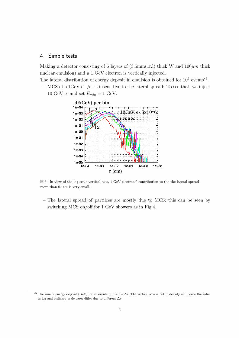
4 Simple tests
Making a detector consisting of 6 layers of (3.5mm(1r.l) thick W and 100µm thick
nuclear emulsion) and a 1 GeV electron is vertically injected.
The lateral distribution of energy deposit in emulsion is obtained for 106 events*5.
– MCS of >1GeV e+/e- is insensitive to the lateral spread: To see that, we inject
10 GeV e- and set Emin = 1 GeV.
dE(GeV) per bin
r (cm)
10GeV e- 5x10^6 events
L=2 4681012
図 3 In view of the log scale vertical axis, 1 GeV electrons’ contribution to the the lateral spread
more than 0.1cm is very small.
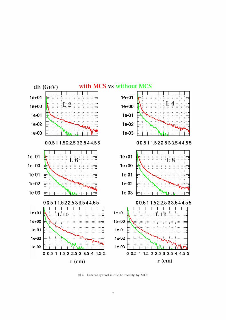
– The lateral spread of partilces are mostly due to MCS: this can be seen by
switching MCS on/off for 1 GeV showers as in Fig.4.
*5 The sum of energy deposit (GeV) for all events in r ∼ r+∆r; The vertical axis is not in density and hence the value
in log and ordinary scale cases differ due to different ∆r.
6
with MCS vs without MCS
L 2 L 4
L 6 L 8
r (cm) r (cm)
dE (GeV)with MCS vs without MCS
L 2 L 4
L 6 L 8
r (cm) r (cm)
dE (GeV)
L 10 L 12
r (cm) r (cm)
with MCS vs without MCSdE (GeV)
図 4 Lateral spread is due to mostly by MCS
7
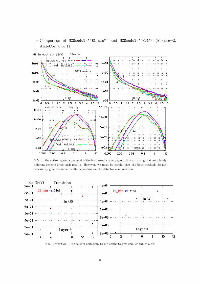
– Comparison of MCSmodel=’"El_hin"’ and MCSmodel=’"Mol"’ (Moliere=2,
AlateCor=0 or 1)
MCSmodel='"El_hin"'
‘Mol’Mol2AL2
10^5 events
1GeV e-dE in each bin (GeV)
L 2
6
10
R(cm)
4
812
R(cm)
same as prev. in log-log
L2 6 10
MCSmodel='"El_hin"'
‘Mol’Mol2AL2
R(cm)
L 4 8 12
R(cm)
図 5 In the entire region, agreement of the both results is very good. It is surprising that completely
different scheme gives such results. However, we must be careful that the both methods do not
necessarily give the same results depending on the detector configuration.
El_hin vs Mol
Layer #
dE (GeV)
In G5
Transition
Layer #
In W
El_hin vs Mol
図 6 Transition. In the thin emulsion, El hin seems to give smaller values a bit.
8
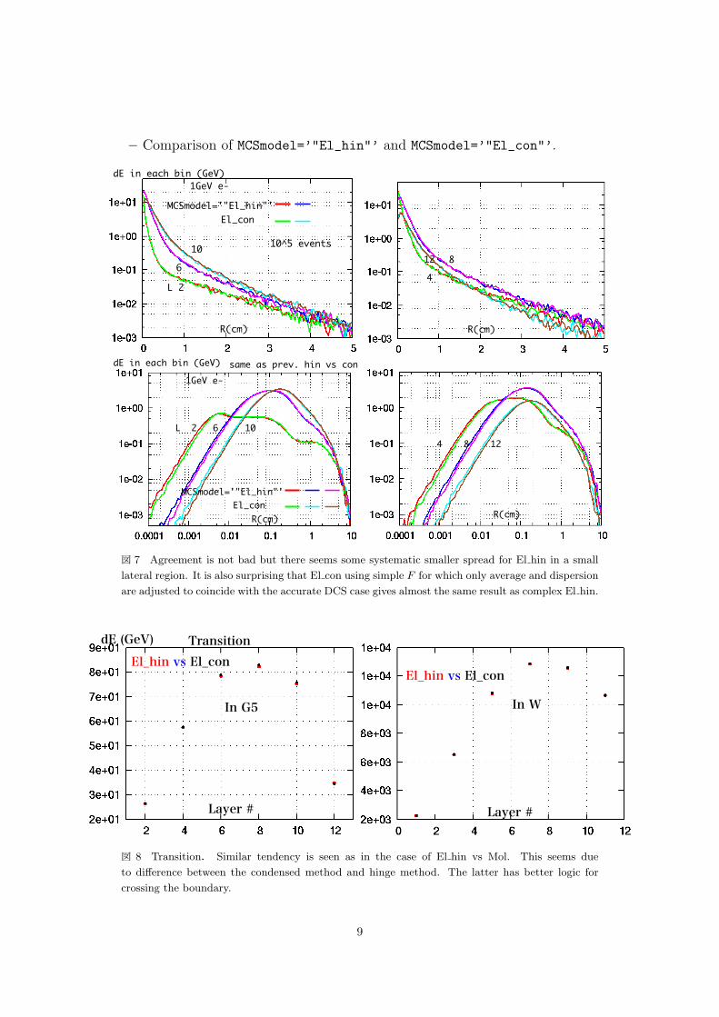
– Comparison of MCSmodel=’"El_hin"’ and MCSmodel=’"El_con"’.
MCSmodel='"El_hin"'El_con
10^5 events
1GeV e-dE in each bin (GeV)
R(cm)
L 2
6
10
R(cm)
4
812
same as prev. hin vs con
MCSmodel='"El_hin"'El_conR(cm)
1GeV e-
dE in each bin (GeV)
L 2 6 10
R(cm)
4 8 12
図 7 Agreement is not bad but there seems some systematic smaller spread for El hin in a small
lateral region. It is also surprising that El con using simple F for which only average and dispersion
are adjusted to coincide with the accurate DCS case gives almost the same result as complex El hin.
El_hin vs El_con
Layer #
dE (GeV)
In G5
Transition
Layer #
In W
El_hin vs El_con
図 8 Transition. Similar tendency is seen as in the case of El hin vs Mol. This seems due
to difference between the condensed method and hinge method. The latter has better logic for
crossing the boundary.
9
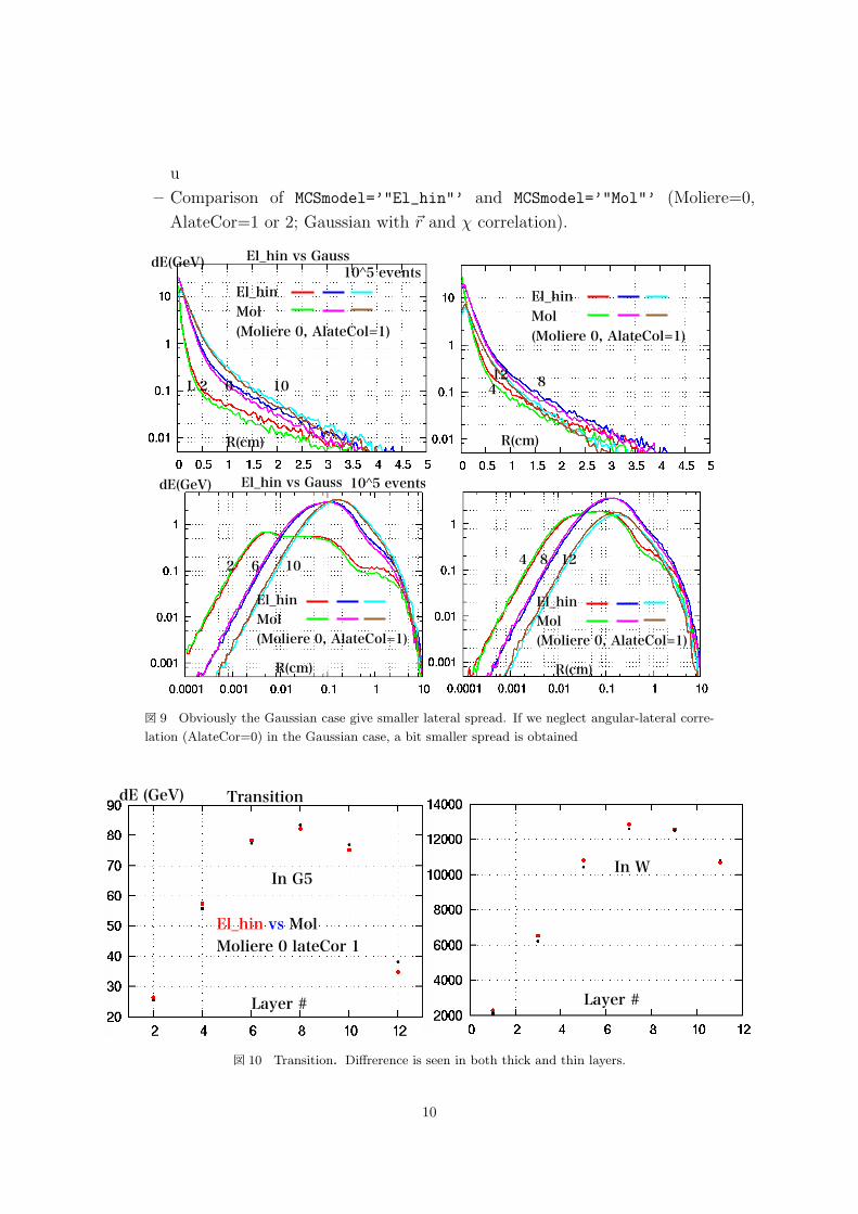
u
– Comparison of MCSmodel=’"El_hin"’ and MCSmodel=’"Mol"’ (Moliere=0,
AlateCor=1 or 2; Gaussian with r and χ correlation).
El_hin vs Gauss
El_hin Mol(Moliere 0, AlateCol=1)
El_hin Mol(Moliere 0, AlateCol=1)
L 2 6 10 4 8 12
R(cm)R(cm)
dE(GeV)10^5 events
El_hin vs Gauss
El_hin Mol(Moliere 0, AlateCol=1)
R(cm)
dE(GeV) 10^5 events
El_hin Mol(Moliere 0, AlateCol=1)
R(cm)
2 6 10 4 8 12
図 9 Obviously the Gaussian case give smaller lateral spread. If we neglect angular-lateral corre-
lation (AlateCor=0) in the Gaussian case, a bit smaller spread is obtained
El_hin vs MolMoliere 0 lateCor 1
Layer #
dE (GeV)
In G5
Transition
Layer #
In W
図 10 Transition.Diffrerence is seen in both thick and thin layers.
10
• Computation time. The El_hin model approaches to the detailed mode as energy
goes lower and need 3 ∼ 4 time more time than other models.
• Comparisons here are very simple. It would be better to compare rigorous El_hin
with Moliere=2 case in actual detector configuration.
For default Moliere setting, Moliere=2 and ALateCor=0 (or 1) is recommended.
For Moliere=2, ALateCor=0 and ALatCor=1 have the same effect (neglect angular-
lateral correlation) and for Moliere=0(Gauss), correlation is taken into account. For
Moliere=1 or 2, ALateCor≤=1 seems better; agreement with El_hin is bit better.
The difference between Moliere=1 and 2 is very small (1 is bit faster; but there is
a report that 2 gives bit better coincidence with experimental data at microscopic
scale distance).
• Data and program place:
The DCS data table is in Cosmos/Data/Elsepa; they are classified by atomic charge
Z and e+ and e-. (∼ 316MB).
The sampling table for Epics application is in Epics/Data/MCS with the same name
as the media file name. (For Cosmos, osmos/Data/MCS/Air).
The MCS model to be used controled in Cosmos/Module/cHowMCS.f90
Programs reaading DCS and TPXS or doing sampling for random processes are in
Cosmos/Particle/Event/Elemag/MixedMCS.
Actural scattering is manged in Epics/prog/epeg.f,epdeflection.f and
Epics/prog/Elemag/epmulScat.f
by using above routines.
If a new medium is introduced (and If El hin or El con is to be used for that medium)
a corresponding data table must be created in Epics/Data/MCS For that, the user
may go to Epics/Util/Elemag/MixedMCS/ and use ./ForManyMeida.sh
It may also be used to make a new table with non-existing parameters. The param-
eters are defined in paramdata file.
Reference
For the mixed simulation and hinge method:
J.M. Femindez-Varea, R. Mayo1, J. Bar and F. Salvat, Nuclear Instruments and Methods
in Physics Research B73 (1993) 447-473.
For the DCS:
Francesc Salvat, Aleksander Jablonski and Cedric J. Powell, Computer Physics Commu-
nications 165 (2005) 157190
11
![doc.: IEEE 802.11-yy/xxxxr0 · Web view14, [2] The fields of the ... The value of this field plus 1 indicates the number of transmit chains used in ... if the Base MCS is MCS 12 or](https://static.fdocument.org/doc/165x107/5ab4a0177f8b9a7c5b8bfe39/doc-ieee-80211-yyxxxxr0-view14-2-the-fields-of-the-the-value-of-this.jpg)