Tomographic phase microscopy

Wonshik Choi, Christopher Fang-Yen, Kamran Badizadegan, Seungeun Oh, Niyom Lue,

Ramachandra R Dasari & Michael S Feld

Supplementary figures and text:

Supplementary Figure 1 Phase projection geometry.

Supplementary Figure 2 Bright field image and index tomogram of C. elegans.

Supplementary Figure 3 Tomogram images from a 30 μm thick suspension of polystyrene

beads.

Supplementary Figure 4 Tomogram images from an 80 μm thick suspension of

polystyrene beads.

Supplementary Methods

Supplementary Software Matlab code for 3-D reconstruction.

Note: Supplementary Video 1 is available on the Nature Methods website.

1

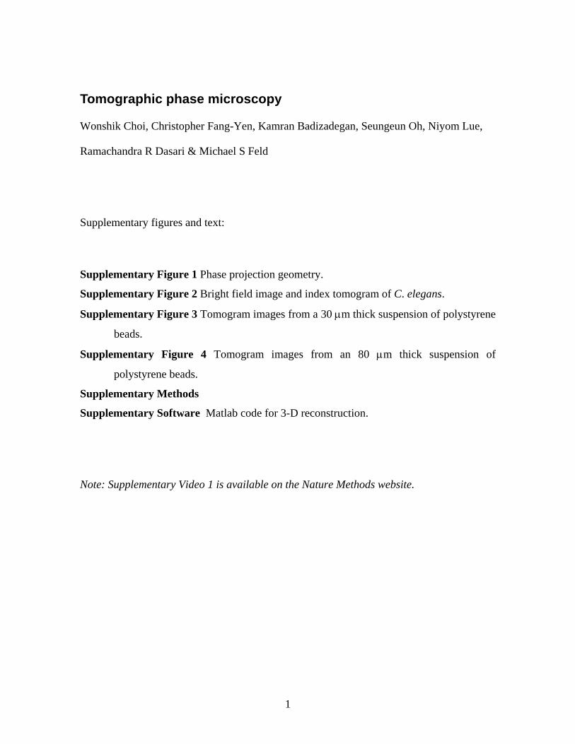
Supplementary Figure 1. Phase projection geometry

(a) Illumination geometry and projection on x-z plane. Blue lines represent the illumination at zero degrees and red lines at angle θ. (b) and (c) Projection phase line profiles of a HeLa cell at θ = 0 and 45 degrees, respectively, at fixed y = y0. (d) and (e) Projection phase images corresponding to (b) and (c), respectively. The color bar indicates the phase in radian. Scale bar, 10μm.

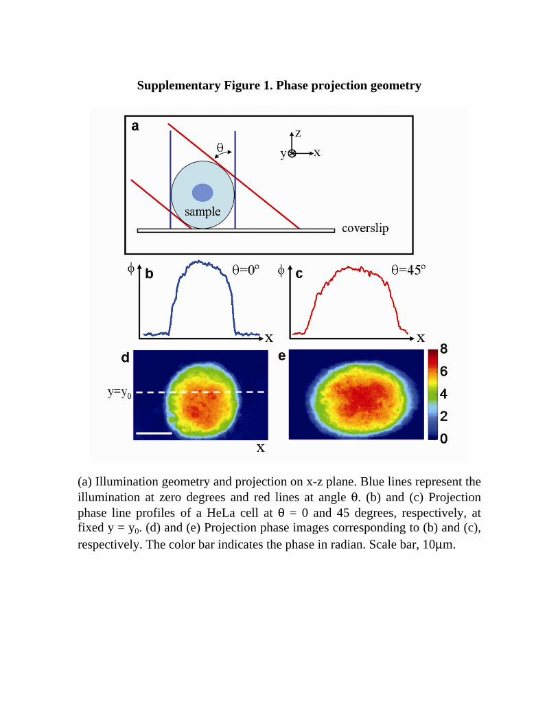
Supplementary Figure 2. Bright field image and index tomogram

of C. elegans.

(a) Mosaic of bright field images of a juvenile C. elegans nematode. (b) Mosaic of x-y slices of index tomograms through center of worm (same as Figure 3d in main text). The color bar indicates the refractive index at λ = 633 nm. Scale bar, 50 µm.

Supplementary Figure 3. Tomogram images from a 30 µm thick

suspension of polystyrene beads

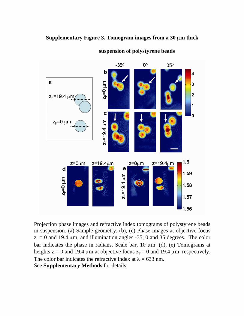
Projection phase images and refractive index tomograms of polystyrene beads in suspension. (a) Sample geometry. (b), (c) Phase images at objective focus zF = 0 and 19.4 µm, and illumination angles -35, 0 and 35 degrees. The color bar indicates the phase in radians. Scale bar, 10 µm. (d), (e) Tomograms at heights z = 0 and 19.4 µm at objective focus zF = 0 and 19.4 µm, respectively. The color bar indicates the refractive index at λ = 633 nm. See Supplementary Methods for details.

Supplementary Figure 4. Tomogram images from an 80 µm thick

suspension of polystyrene beads

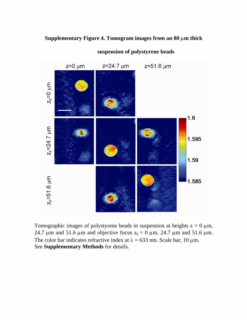
Tomographic images of polystyrene beads in suspension at heights z = 0 µm, 24.7 µm and 51.6 µm and objective focus zF = 0 µm, 24.7 µm and 51.6 µm. The color bar indicates refractive index at λ = 633 nm. Scale bar, 10 µm. See Supplementary Methods for details.

Supplementary methods

Bright field and fluorescence imaging

The tomographic phase microscope is also designed to accommodate bright field

and fluorescence imaging. For bright field imaging, a white light emitting diode (LED)

placed between the scanning mirror and a condenser lens serves as an illuminator, and

images are recorded by a CCD camera (Photometric CoolSnap HQ) along a separate

optical path (not shown in Fig. 1). Bright field images provide a form of optical

sectioning, due to the extremely short depth of field (<1 µm) provided by NA 1.4

illumination and collection. For fluorescence imaging, a standard filter cube (Olympus)

with appropriate filters is placed under the objective lens, and fluorescence excitation is

provided by either a mercury arc lamp (Olympus) or a collimated blue LED (Lumileds).

For single cells, widefield fluorescence imaging using DAPI or SYTO (Invitrogen)

nucleic acid stains is used to identify nuclear boundaries.

Laser interferometer phase measurement

In the interferometer sample arm, the beam is incident on a tilting mirror

controlled by a galvanometer (HS-15, Nutfield technology) (Fig. 1). A lens (L1, f =

250mm) is used to focus the beam at the back focal plane of an oil-immersion condenser

lens (Nikon 1.4NA), which recollimates the beam to a diameter of approximately 600 µm.

The distances from tilting mirror to the lens (L1) and from the lens (L1) to the back focal

plane of the condenser lens are set equal to the focal length of the lens (L1) such that the

tilting mirror is conjugate to the sample plane.

Samples are prepared in chambers composed of two glass coverslips separated by

a plastic spacer ring and partially sealed with adhesive. Light transmitted through the

sample is collected by an infinity-corrected, oil-immersion objective lens (Olympus

UPLSAPO 100XO, 1.4 NA). A tube lens (L2, f = 200 mm) focuses an image of the

sample onto the camera plane with magnification M=110.

In the reference arm, the laser beam passes through two acousto-optic modulators

(AOMs) (Isomet) driven at frequencies ω1 = 110.1250 MHz and ω2= 110.0000 MHz,

respectively, using a custom-built digitally synthesized RF driver. Irises select the +1

and -1 order beams, respectively, such that the total reference beam frequency shift is

1250 Hz. After passing through the AOMs, the reference beam is spatial filtered and

enlarged by a beam expander.

A beamsplitter recombines the sample and reference laser beams, forming an

interference image at the camera plane. The focus and tilt of sample and reference beams

are adjusted to minimize the difference between the two wavefronts.

For each phase image, a high speed CMOS camera (Photron 1024-PCI, 17µm

pixel size) records 4 images separated by 200 µs, exactly one-quarter the reciprocal of the

heterodyne frequency. In this way, four interference patterns I1, I2, I3, I4 are recorded in

which the sample-reference phase shift between consecutive images differs by π/2.

Phase images are then obtained by applying phase shifting interferometry using the four-

bucket algorithm1 φ(x,y)=arg (((I4-I2) + i(I3-I1)). 2π-phase ambiguities are resolved by

phase unwrapping using Goldstein’s algorithm2. The fast acquisition time between

frames reduces the effects of external noise. Exposure times are typically ~20 µs. By

stepping the galvanometer mirror, 81 phase images are recorded for sample illumination

angles θ = -60 to +60 degrees in steps of 1.5 degrees.

The phase projection geometry is shown in Supplementary Figure 1, illustrated

by data from a single HeLa cell in a culture medium (DMEM with 10% fetal bovine

serum). The phase image of the cell for θ = 0 degree is shown in Supplementary Figure

1d. For nonzero θ the image displays a background fringe pattern due to the tilt between

sample and reference beams, with fringe spacing d = λ M/(n sin θ), with M = 110 the

magnification and n the index of the sample medium (image next to the camera in Figure

1 of the main text). The corresponding phase image shows a 2π jump at every fringe.

After unwrapping the phase, the phase image appears as a nearly linear phase ramp with

the phase profile of the cell almost indistinguishable.

The phase image at an illumination angle of 45o is shown in Supplementary

Figure 1e after phase unwrapping and subtraction of the background phase ramp via a

least-square linear fit to a portion of the field of view with no sample. Compared to the

zero degree angle case (Supplementary Fig. 1b), the line profile of the phase image is

elongated at nonzero illumination (Supplementary Fig. 1c), because the phase

measurements are performed in an image plane parallel to the sample substrate,

regardless of incident beam direction (Supplementary Fig. 1a).

A similar angle-dependent set of phase images is obtained with no sample present,

and the resulting set of background phase images is subtracted from the sample phase

images to eliminate residual fixed-pattern phase noise due to optical aberrations and

imperfect alignment.

Iterative constraint algorithm

The limitation of projection angles to |θ| < 60 degrees poses a problem of missing

information. There have been many computed tomography studies addressing limited

angle problems3-5. To reduce the effect of the missing projections, we applied an iteration

based constraint method5. In this technique, the reconstruction is first performed by

filling missing-angle projections with values of zero. The resulting reconstructed image,

which represents the difference of the refractive index relative to that of the surrounding

medium, is constrained to contain only non-negative values and set to zero outside some

boundary chosen well outside the margins of the cell. Next, a θ-dependent projection of

this reconstruction is calculated and constrained to equal experimentally measured

projections over the range of measured angles θ. The process is repeated 10-15 times to

ensure convergence.

Absolute index calibration

Since all phase measurements in this experiment are measured relative to other

points in the field of view, the tomographic data from the algorithm gives the refractive

index relative to that of the medium. The absolute index was calculated by adding the

relative index to the index of refraction of the culture medium, found to be 1.337 using a

different interferometric method6.

Imaging thick samples

The measurement of 3-D refractive index will allow quantitative characterization

of sample-induced aberrations. Such aberrations become progressively more severe for

thicker tissues, although recent work has shown that biological structures ~30 µm thick

can induce significant optical aberrations7. We therefore explored methods for imaging

samples much thicker than single cell layers.

Our reconstruction algorithm approximates the phase of the sample field as the

integral of refractive index along a straight line in the direction of beam propagation. We

refer to this as the projection approximation; it is also known as the eikonal or ray

approximation. The projection approximation places constraints not only on the index

variations of the sample but also its thickness. For plane wave illumination of a typical

cell, the projection approximation is accurate to depths of roughly 15 microns. To address

this limitation, we have explored the use of focusing at multiple planes to extend the

range of tomographic imaging.

We prepared test samples composed of 10 µm polystyrene beads (Polysciences)

suspended in UV-curable optical adhesive (Norland or Dymax) and sandwiched between

two glass coverslips (Supplementary Fig. 3a). Projection phase images at three different

angles of illumination (-35o, 0o and 35o) for two different positions of the objective focus

(zF = 0 µm and zF = 19.4 µm) are shown in Supplementary Figure 3b-c. In

Supplementary Figure 3c, the in-focus bead (white arrow) is clearly resolved and

satisfies the projection approximation while the out-of-focus beads exhibit ring patterns

due to diffraction, demonstrating the breakdown of the projection approximation. Note

that for both focus positions, in-focus beads (white arrows) are stationary with respect to

change in illumination angle, while out-of-focus beads are not. This angle-dependent

position information is the basis of depth discrimination in our tomographic

reconstruction algorithm; the in-focus beads are separated in height from the defocused

beads although all beads are present in the phase images.

In Supplementary Figure 3d, x-y slices of the resulting tomogram at the centers

of an in-focus bead (z = 0 µm) and defocused bead (z = 19.4 µm) are shown at an

objective focus zF = 0 µm. The same slices for zF = 19.4 µm are shown in

Supplementary Figure 3e. The in-focus beads, which satisfy the projection

approximation in the phase images, are clearly resolved in the tomograms, while out-of-

focus beads are blurred and exhibit ring pattern artifacts. Similar results are obtained in

test samples up to 80 µm thick. In Supplementary Figure 4, three focal depths are used

to measure tomograms centered at three beads, with a 51 µm separation between the

highest and lowest. The signal-to-noise ratio is somewhat lower in this data, due to the

smaller refractive index contrast between beads and adhesive.

These results suggest a simple scheme for measuring samples of extended

thickness, in which the objective focus is automatically scanned over intervals of 15µm

(or less) to cover the sample depth and obtain a set of tomograms at each step of the focus.

By combining in-focus slices in series, a mosaic tomogram covering the entire sample

can then be created. The maximum thickness of samples is then limited not by the

projection approximation but by other factors, such as sample absorption, light scattering

and the objective working distance.

Data collection and analysis

Experiment control, data acquisition, data processing and image display were

done using MATLAB software (Mathworks Inc.). Data analysis code is given in

Supplementary Software 1.

References

1. Creath, K. Progress in Optics 26, 349-393 (1988). 2. Goldstein, R. M., Zebker, H. A. & Werner, C. L. Radio Science 23, 713-720

(1988). 3. Kawata, S., Nakamura, O. & Minami, S. J. Opt. Soc. Am. A 4, 292-297 (1987). 4. Medoff, B. P., Brody, W. R., Nassi, M. & Macovski, A. J. Opt. Soc. Am. 73,

1493-1500 (1983). 5. Perez-Mendez, K. C. T. a. V. J. Opt. Soc. Am. 71, 582 (1981). 6. Lue, N. et al. Opt. Lett. 31, 2759-2761 (2006). 7. Schwertner, M., Booth, M. J. & Wilson, T. Opt. Express 12, 6540-6552 (2004).

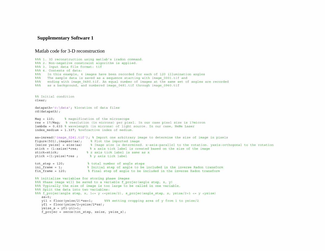
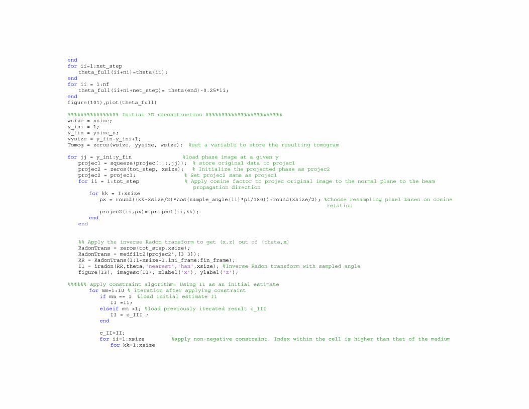
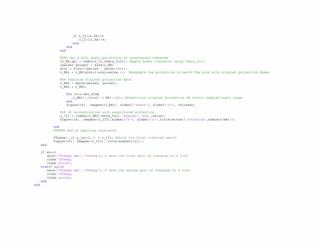
Supplementary Software 1

Matlab code for 3-D reconstruction %%% 1. 3D reconstruction using matlab’s iradon command. %%% 2. Non-negative constraint algorithm is applied. %%% 3. Input data file format: tif %%% 4. Contents of data: %%% In this example, 4 images have been recorded for each of 120 illumination angles %%% The sample data is saved as a sequence starting with image_0001.tif and %%% ending with image_0480.tif. An equal number of images at the same set of angles are recorded %%% as a background, and numbered image_0481.tif through image_0960.tif %% Initial condition clear; datapath='c:\data'; %location of data files cd(datapath); Mag = 110; % magnification of the microscope res = 17/Mag; % resolution (in microns) per pixel. In our case pixel size is 17micron lambda = 0.633 % wavelength (in microns) of light source. In our case, HeNe Laser index_medium = 1.337; %refractive index of medium. aa=imread('image_0241.tif'); % Import one arbitrary image to determine the size of image in pixels figure(501),imagesc(aa); % Plot the imported image [xsize ysize] = size(aa) % Image size is determined. x-axis:parallel to the rotation. yaxis:orthogonal to the rotation xtick = (1:xsize)*res; % x axis tick label is created based on the size of the image ztick=xtick; % z axis tick label is same as x ytick =(1:ysize)*res ; % y axis tick label tot_step = 120; % total number of angle steps ini_frame = 1; % Initial step of angle to be included in the inverse Radon transform fin_frame = 120; % Final step of angle to be included in the inverse Radon transform %% initialize variables for storing phase images %%% Phase image will be saved to a variable f_projec(angle step, x, y) %%% Typically the size of image is too large to be called in one variable. %%% Split the data into two variables: %%% f_projec(angle step, x, 1<= y <=ysize/2), s_projec(angle_step, x, ysize/2+1 <= y <ysize) ss=0; yi1 = floor(ysize/2)*ss+1; %%% setting cropping area of y from 1 to ysize/2 yf1 = floor(ysize/2+ysize/2*ss); ysize_s = yf1-yi1+1; f_projec = zeros(tot_step, xsize, ysize_s);

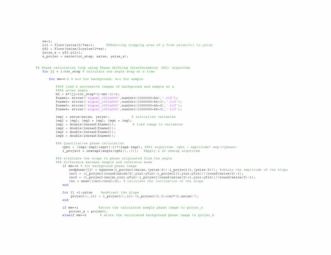
ss=1; yi2 = floor(ysize/2)*ss+1; %%%setting cropping area of y from ysize/2+1 to ysize yf2 = floor(ysize/2+ysize/2*ss); ysize_s = yf2-yi2+1; s_projec = zeros(tot_step, xsize, ysize_s); %% Phase calculation loop using Phase Shifting Interferometry (PSI) algorithm for jj = 1:tot_step % calculate one angle step at a time for mm=0:1 % m=0 for background, m=1 for sample %%%% load 4 successive images of background and sample at a %%%% given angle kk = 4*(jj+tot_step*(1-mm)-1)+1; fname1= strcat('signal_c001s000',num2str(1000000+kk),'.tif'); fname2= strcat('signal_c001s000',num2str(1000000+kk+1),'.tif'); fname3= strcat('signal_c001s000',num2str(1000000+kk+2),'.tif'); fname4= strcat('signal_c001s000',num2str(1000000+kk+3),'.tif'); img1 = zeros(xsize, ysize); % initialize variables img2 = img1; img3 = img1; img4 = img1; img1 = double(imread(fname1)); % load image to variables img2 = double(imread(fname2)); img3 = double(imread(fname3)); img4 = double(imread(fname4)); %%% Quantitative phase calculation cphi = (img1-img3)+sqrt(-1)*(img4-img2); %PSI algorithm. cphi = amplitude* exp(i*phase). i_projec1 = unwrap2(angle(cphi(:,:))); %Apply a 2D unwrap algorithm %%% eliminate the slope in phase originated from the angle %%% difference between sample and reference beam if mm==0 % for background phase image endphase(jj) = squeeze(i_projec1(xsize,(ysize-2))-i_projec1(1,(ysize-2))); %obtain the amplitude of the slope inc1 = (i_projec1(round(xsize/2),yini:yfin)-i_projec1(1,yini:yfin))/(round(xsize/2)-1); inc2 = (i_projec1(xsize,yini:yfin)-i_projec1(round(xsize/2)+1,yini:yfin))/(round(xsize/2)-1); inc = mean((inc1+inc2)/2); % calculate the inclination of the slope end for ll =1:ysize %subtract the slope projec1(:,ll) = i_projec1(:,ll)-(i_projec1(1,1)+inc*(1:xsize)'); end if mm==1 %store the calculated sample phase image to projec_s projec_s = projec1; elseif mm==0 % store the calculated background phase image to projec_b

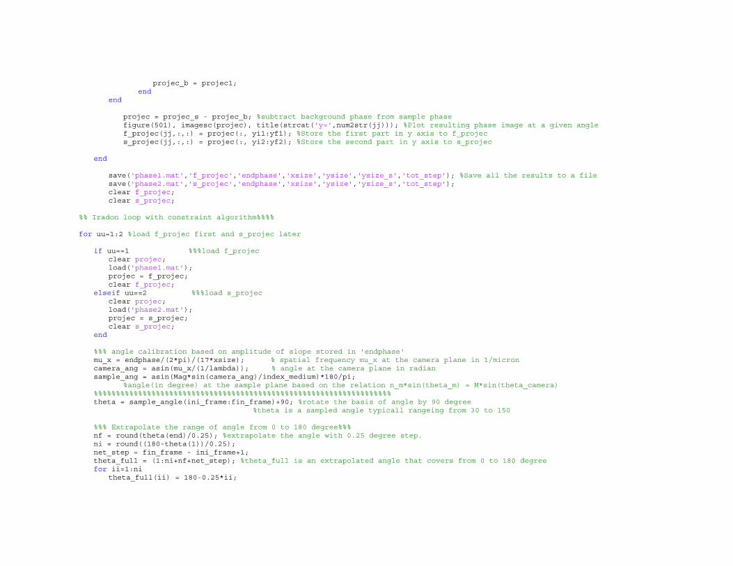
projec_b = projec1; end end projec = projec_s - projec_b; %subtract background phase from sample phase figure(501), imagesc(projec), title(strcat('y=',num2str(jj))); %Plot resulting phase image at a given angle f_projec(jj,:,:) = projec(:, yi1:yf1); %Store the first part in y axis to f_projec s_projec(jj,:,:) = projec(:, yi2:yf2); %Store the second part in y axis to s_projec end save('phase1.mat','f_projec','endphase','xsize','ysize','ysize_s','tot_step'); %Save all the results to a file save('phase2.mat','s_projec','endphase','xsize','ysize','ysize_s','tot_step'); clear f_projec; clear s_projec; %% Iradon loop with constraint algorithm%%%% for uu=1:2 %load f_projec first and s_projec later if uu==1 %%%load f_projec clear projec; load('phase1.mat'); projec = f_projec; clear f_projec; elseif uu==2 %%%load s_projec clear projec; load('phase2.mat'); projec = s_projec; clear s_projec; end %%% angle calibration based on amplitude of slope stored in 'endphase' mu_x = endphase/(2*pi)/(17*xsize); % spatial frequency mu_x at the camera plane in 1/micron camera_ang = asin(mu_x/(1/lambda)); % angle at the camera plane in radian sample_ang = asin(Mag*sin(camera_ang)/index_medium)*180/pi; %angle(in degree) at the sample plane based on the relation n_m*sin(theta_m) = M*sin(theta_camera) %%%%%%%%%%%%%%%%%%%%%%%%%%%%%%%%%%%%%%%%%%%%%%%%%%%%%%%%%%%%%%%%%%% theta = sample_angle(ini_frame:fin_frame)+90; %rotate the basis of angle by 90 degree %theta is a sampled angle typicall rangeing from 30 to 150 %%% Extrapolate the range of angle from 0 to 180 degree%%% nf = round(theta(end)/0.25); %extrapolate the angle with 0.25 degree step. ni = round((180-theta(1))/0.25); net_step = fin_frame - ini_frame+1; theta_full = (1:ni+nf+net_step); %theta_full is an extrapolated angle that covers from 0 to 180 degree for ii=1:ni theta_full(ii) = 180-0.25*ii;

end for ii=1:net_step theta_full(ii+ni)=theta(ii); end for ii = 1:nf theta_full(ii+ni+net_step)= theta(end)-0.25*ii; end figure(101),plot(theta_full) %%%%%%%%%%%%%%%% Initial 3D reconstruction %%%%%%%%%%%%%%%%%%%%%%%% wsize = xsize; y_ini = 1; y_fin = ysize_s; yysize = y_fin-y_ini+1; Tomog = zeros(wsize, yysize, wsize); %set a variable to store the resulting tomogram for jj = y_ini:y_fin %load phase image at a given y projec1 = squeeze(projec(:,:,jj)); % store original data to projec1 projec2 = zeros(tot_step, xsize); % Initialize the projected phase as projec2 projec2 = projec1; % Set projec2 same as projec1 for ii = 1:tot_step % Apply cosine factor to projec original image to the normal plane to the beam

propagation direction for kk = 1:xsize px = round((kk-xsize/2)*cos(sample_angle(ii)*pi/180))+round(xsize/2); %Choose resampling pixel basen on cosine

relation projec2(ii,px)= projec1(ii,kk); end end %% Apply the inverse Radon transform to get (x,z) out of (theta,x) RadonTrans = zeros(tot_step,xsize); RadonTrans = medfilt2(projec2',[3 3]); RR = RadonTrans(1:1+xsize-1,ini_frame:fin_frame); I1 = iradon(RR,theta,'nearest','han',xsize); %Inverse Radon transform with sampled angle figure(13), imagesc(I1), xlabel('x'), ylabel('z'); %%%%%% apply constraint algorithm: Using I1 as an initial estimate for mm=1:10 % iteration after applying constraint if mm == 1 %load initial estimate I1 II =I1; elseif mm >1; %load previously iterated result c_III II = c_III ; end c_II=II; for ii=1:xsize %apply non-negative constraint. Index within the cell is higher than that of the medium for kk=1:xsize

if c_II(ii,kk)<0 c_II(ii,kk)=0; end end end %%%% Get a full angle projection of constrained tomogram [c_RR,xp] = radon(c_II,theta_full); %Apply Radon transform using theta_full [xsize2 ysize2] = size(c_RR) xini = floor((xsize2 - xsize)/2+1); c_RR1 = c_RR(xini+1:xini+xsize,:); %Resample the projection to match the size with original projection phase %%% Subtitue original projection data c_RR2 = zeros(xsize2, ysize2); c_RR2 = c_RR1; for ii=1:net_step c_RR2(:,ii+ni) = RR(:,ii); %Substitute original projection RR within sampled angle range end figure(16), imagesc(c_RR2), xlabel('theta'), ylabel('x'), colorbar; %%% 3D reconstruction with substituted projection c_III = iradon(c_RR2,theta_full,'nearest','han',xsize); figure(14), imagesc(c_III),xlabel('x'), ylabel('z'),title(strcat('iteration',num2str(mm))); end %%%%%% end of applying constraint CTomog(:,jj-y_ini+1,:) = c_III; %Store the final iterated result figure(15), imagesc(c_III), title(num2str(jj)); end if uu==1 save('CTomog1.mat','CTomog'); % save the first part of tomogram to a file clear CTomog; clear projec; elseif uu==2 save('CTomog2.mat','CTomog'); % save the second part of tomogram to a file clear CTomog; clear projec; end end