Statistics for Particle Physics: Intervals

Roger BarlowKarlsruhe: 12 October 2009

Summary

Techniques• ΔΧ2=1, Δln L=-½• 1D and 2+D• Integrating and/or

profiling

Karlsruhe: 12 October 2009 Roger Barlow: Intervals and Limits 2

Concepts• Confidence and

Probability• Chi squared• p-values• Likelihood• Bayesian Probability

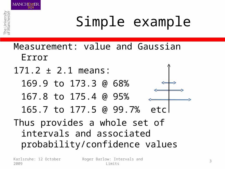
Simple example

Measurement: value and Gaussian Error171.2 ± 2.1 means:

169.9 to 173.3 @ 68%167.8 to 175.4 @ 95%165.7 to 177.5 @ 99.7% etc

Thus provides a whole set of intervals and associated probability/confidence values

Karlsruhe: 12 October 2009 Roger Barlow: Intervals and Limits 3

Aside (1): Why Gaussian?

Central Limit Theorem:The cumulative effect of many different

uncertainties gives a Gaussian distribution – whatever the form of the constituent distributions.

Moral: don’t worry about nonGaussian distributions. They will probably be combined with others.

Karlsruhe: 12 October 2009 Roger Barlow: Intervals and Limits 4

Aside(2) Probability and confidence

“169.9 to 173.3 @ 68%”What does this mean? Number either is in this

interval or it isn’t. Probability is either 0 or 1. This is not like population statistics.

Reminder: basic definition of probability as limit of frequency P(A)= Limit N(A)/N

Interpretation. ‘The statement “Q lies in the range 169.9 to 173.3” has a 68% probability of being true.’ Statement made with 68% confidence

Karlsruhe: 12 October 2009 Roger Barlow: Intervals and Limits 5

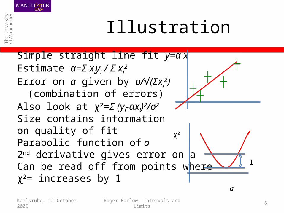
IllustrationSimple straight line fit y=a xEstimate a=Σ xiyi / Σ xi

2

Error on a given by σ/√(Σxi2)

(combination of errors)Also look at χ2=Σ (yi-axi)2/σ2

Size contains information on quality of fit Parabolic function of a2nd derivative gives error on aCan be read off from points where χ2= increases by 1

Karlsruhe: 12 October 2009 Roger Barlow: Intervals and Limits 6

a

χ2

1

Illustration

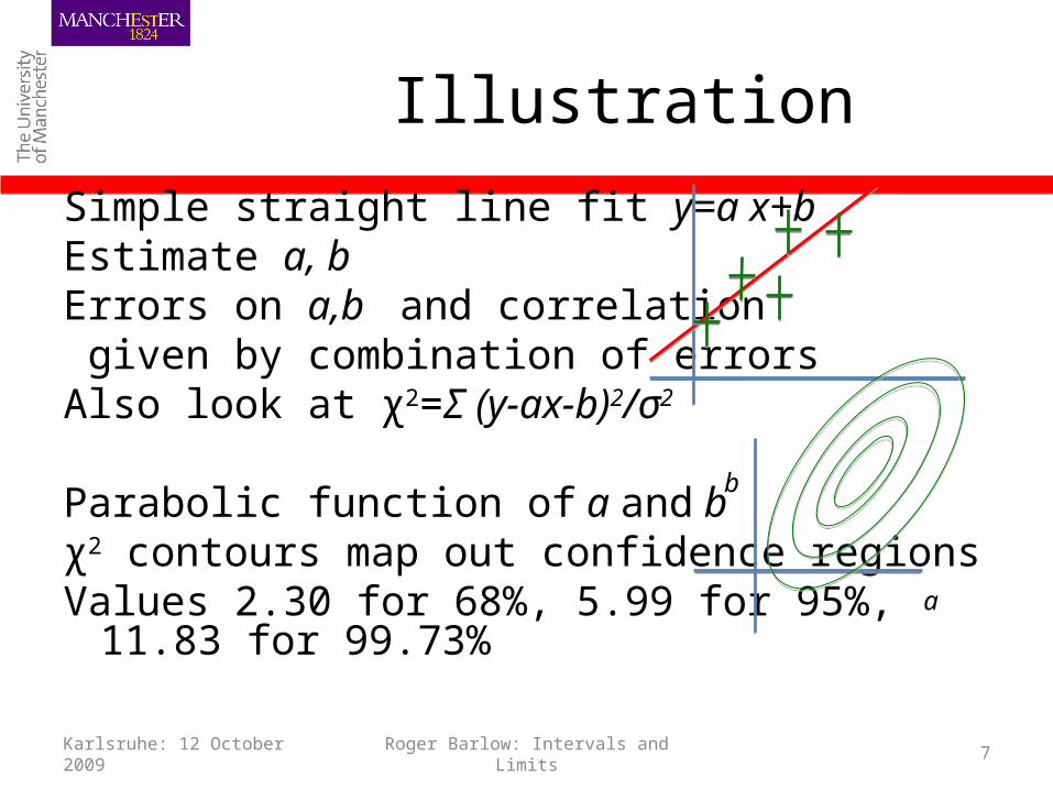
Simple straight line fit y=a x+bEstimate a, b Errors on a,b and correlation given by combination of errorsAlso look at χ2=Σ (y-ax-b)2/σ2

Parabolic function of a and b χ2 contours map out confidence regionsValues 2.30 for 68%, 5.99 for 95%, 11.83 for 99.73%

Karlsruhe: 12 October 2009 Roger Barlow: Intervals and Limits 7

a

b

χ2

Χ2 Distribution is convolution of N Gaussians

Expected χ2 ≈N If χ2 >> N the model is implausible.

Quantify this using standard function F(χ2 ;N) Fitting a parameter just reduces N by 1

Karlsruhe: 12 October 2009 Roger Barlow: Intervals and Limits 8

Chi squared probability and p values

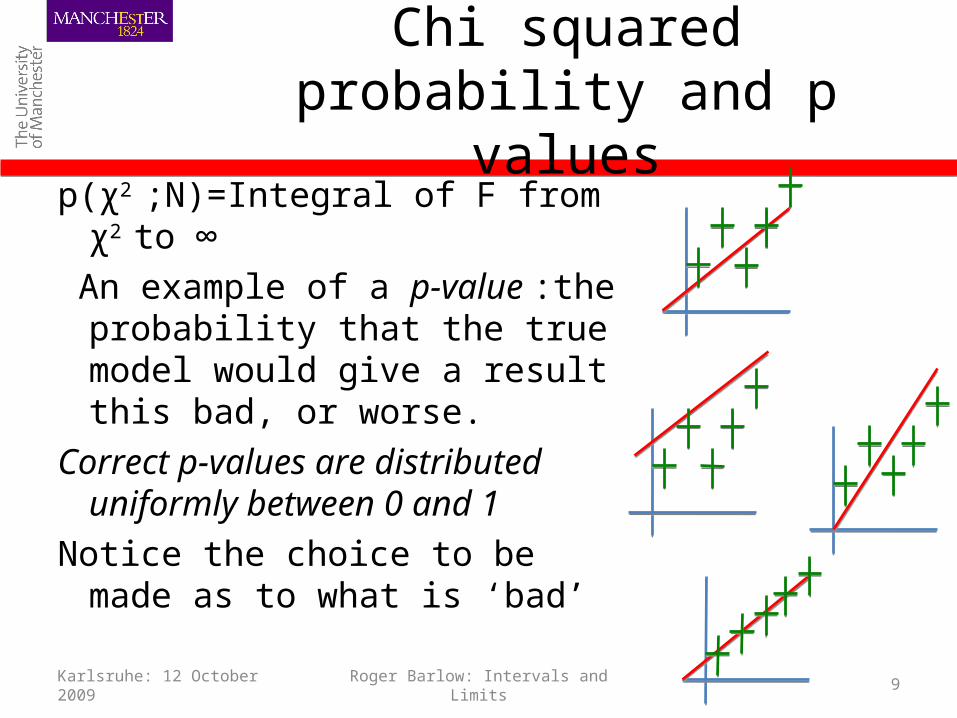
p(χ2 ;N)=Integral of F from χ2 to ∞ An example of a p-value :the

probability that the true model would give a result this bad, or worse.

Correct p-values are distributed uniformly between 0 and 1

Notice the choice to be made as to what is ‘bad’

Karlsruhe: 12 October 2009 Roger Barlow: Intervals and Limits 9

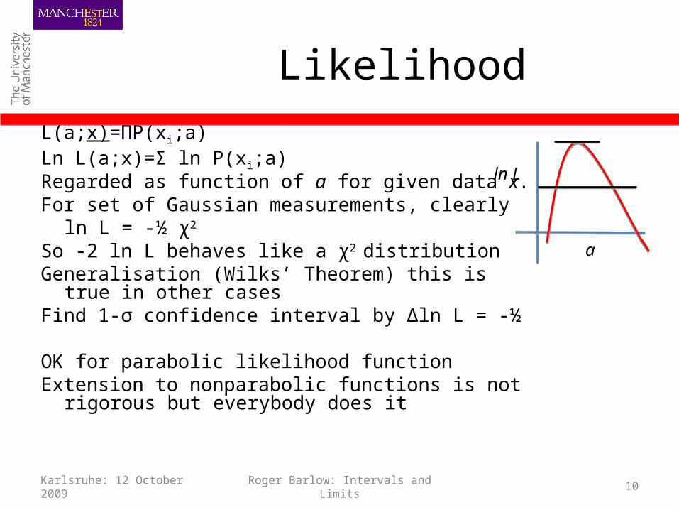
LikelihoodL(a;x)=ΠP(xi;a)Ln L(a;x)=Σ ln P(xi;a)Regarded as function of a for given data x.For set of Gaussian measurements, clearly

ln L = -½ χ2

So -2 ln L behaves like a χ2 distribution Generalisation (Wilks’ Theorem) this is true in other casesFind 1-σ confidence interval by Δln L = -½

OK for parabolic likelihood functionExtension to nonparabolic functions is not rigorous but

everybody does it

Karlsruhe: 12 October 2009 Roger Barlow: Intervals and Limits 10

a

ln L

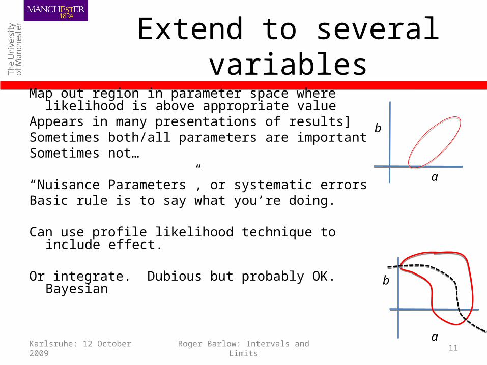
Extend to several variablesMap out region in parameter space where likelihood is

above appropriate valueAppears in many presentations of results]Sometimes both/all parameters are importantSometimes not…

“Nuisance Parameters”, or systematic errorsBasic rule is to say what you’re doing.

Can use profile likelihood technique to include effect. Or integrate. Dubious but probably OK. Bayesian

Karlsruhe: 12 October 2009 Roger Barlow: Intervals and Limits 11

a

b

a

b

Bayes theorem

P(A|B) = P(B|A) P(A) P(B)Example: Particle ID

Bayesian ProbabilityP(Theory|Data) = P(Data|Theory) P(Theory) P(Data)Example: bets on tossing a coinP(Theory): Prior P(Theory|Data): PosteriorApparatus all very nice but prior is subjective.

Karlsruhe: 12 October 2009 Roger Barlow: Intervals and Limits 12

Bayes and distributions

Extend method. For parameter a have prior probability distribution P(a) and then posterior probability distribution P(a|x)

Intervals can be read off directly.In simple cases, Bayesian and frequentist

approach gives the same results and there is no real reason to use a Bayesian analysis.

Karlsruhe: 12 October 2009 Roger Barlow: Intervals and Limits 13

Nuisance parameters

L(a,b;x) and b is of no interest (e.g. experimental resolution).

May have additional knowledge e.g. from another channel

L’(a;x)=∫L(a,b;x) P(b) dbSeems natural – but be careful

Karlsruhe: 12 October 2009 Roger Barlow: Intervals and Limits 14

Summary

Techniques• ΔΧ2=1, Δln L=-½• 1D and 2+D• Integrating and/or

profiling

Karlsruhe: 12 October 2009 Roger Barlow: Intervals and Limits 15

Concepts• Confidence and

Probability• Chi squared• p-values• Likelihood• Bayesian Probability