SPE-174068-MS

Using Wireline Standoffs (WLSOs) To Mitigate Cable Sticking G.Wheater, Gaia Earth Sciences Limited; Lee Paterson, Ben Kidd, BHP Billiton plc; Rob MacLeod, Nexen Petroleum USA Inc.; Stuart Huyton, Luke Miller, Lee Hyson, Matt Sauder, Gaia Earth Sciences Limited; and Bill Morris, John Hall, Impact Selector Inc. All SPE.

Copyright 2015, Society of Petroleum Engineers This paper was prepared for presentation at the SPE Western Regional Meeting held in Garden Grove, California, USA, 27–30 April 2015. This paper was selected for presentation by an SPE program committee following review of information contained in an abstract submitted by the author(s). Contents of the paper have not been reviewed by the Society of Petroleum Engineers and are subject to correction by the author(s). The material does not necessarily reflect any position of the Society of Petroleum Engineers, its officers, or members. Electronic reproduction, distribution, or storage of any part of this paper without the written consent of the Society of Petroleum Engineers is prohibited. Permission to reproduce in print is restricted to an abstract of not more than 300 words; illustrations may not be copied. The abstract must contain conspicuous acknowledgment of SPE copyright.

Abstract

The recent development of wireline standoffs (WLSOs) has effectively eliminated cable sticking during

deepwater logging operations, offering a viable alternative to pipe-conveyed logging, and saving

considerable rig time and risk in the process. On eight high overbalance wells in the Gulf of Mexico,

multiple arrays of wireline standoffs (WLSOs) have been successfully deployed to facilitate deep formation

sampling without any incidence of cable sticking. This success should be viewed in the context of the fact

that the cable force modeling for WLSO deployment indicated that several fishing operations were averted.

The oil and gas industry has been using standoffs for years in order to prevent sticking of everything from

logging tools to casing. Applying standoff technology to logging cable was a natural progression, although

there were many technical challenges that needed to be overcome in order to make the effective use of

WLSOs a reality. To begin, the wireline standoffs could not be allowed to damage the logging cable. Yet,

these standoffs had to provide a grip sufficient to avoid slippage under high tensions. In addition, the

WLSOs needed to be capable of both maximum cable lift and minimal formation contact, while allowing

a 3-3/8” fishing grapple to smoothly pass over them. Finally, WLSO modeling had to be able to identify

their optimal placement on the cable, taking into account such factors as logging objectives, wellbore

trajectory, and applied cable forces (including cable sag between WLSOs in deviated holes).

This paper discusses the origins of WLSO design, job planning, and operating procedures.

Recommendations for future research into the issue of cable sticking are also included.

Introduction & Background

A comprehensive study of formation tester sticking modes for the Gulf Coast region determined that about

70% of sticking events from a total of 664 jobs studied involved stuck cable (Underhill, Moore, & Meeten,

1998). In another study of 295 jobs (region unspecified), it was reported that the use of wireline jars

drastically reduced the overall fishing rate. However, 11% of the jobs still required fishing operations. It

should be noted that 50% of those 11% of jobs required fishing because of stuck cable (Evans, Brame, &

Rose, 2007).

2 SPE-174068-MS

There have been a number of advances in wireline conveyance modeling, technologies, and techniques in

recent years (Sarian, Varkey, Protasov, & Turner, 2013; Prasad, Castillo, & Elshahawi, 2012; Castillo &

Wills, 2007; Evans, Brame, & Rose, 2007). However, it could be argued that diagnosing and mitigating

cable sticking has not generally received the focus it has deserved. Stuck cable can have a serious impact

on the AFE. If the cable does not pull free, then drill pipe must be deployed to strip over the line and run

past the stuck point. This intervention can be very costly, consuming 1 – 4 days of rig time, depending on

well depth, stuck point, and fishing method. Cable sticking can also diminish the capacity to free log tools

with wireline jars, since either firing or re-cocking can be compromised. A focus on cable sticking

mitigation is therefore warranted, with the goal of minimizing the overall sticking risk, reducing NPT from

fishing, and matching the other recent developments and innovations in wireline conveyance.

Differential sticking mechanisms and modeling

It should be noted at the outset that this paper does not explore the complex science of mud cake generation,

composition, and sticking capacity, which has been studied in great detail by others (Dupriest, Jr, &

Ottesen, 2011; P. Isambourg, 1999; Reid, et al., 1996). The aim of this paper is to explore the impact of

differential sticking on overall wireline conveyance, as well as to address the mitigation of cable sticking

through the deployment of WLSOs. To begin with the basics:

In simplest form, the force acting on an object of area A, from differential pressure ΔP is:

F = ΔP x A,……………………(Eq.1)

Consequently, a “Pull to Free” force is required to overcome the sticking:

Pull to Free (PTF) = µ x ΔP x A,….……………….(Eq.2)

Where: µ = sticking coefficient

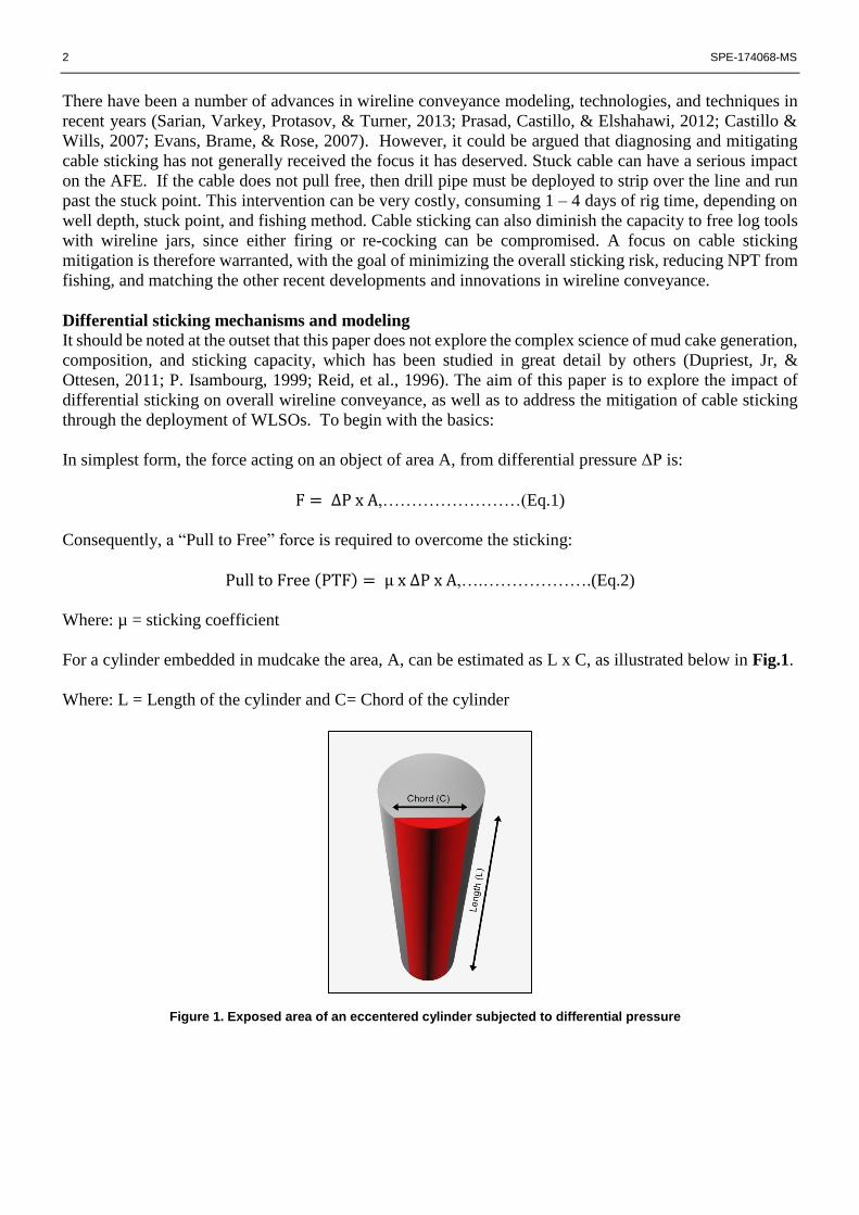
For a cylinder embedded in mudcake the area, A, can be estimated as L x C, as illustrated below in Fig.1.

Where: L = Length of the cylinder and C= Chord of the cylinder

Figure 1. Exposed area of an eccentered cylinder subjected to differential pressure

SPE-174068-MS 3

The only verifiable component (at downhole conditions) in Eq. 2 is ΔP. Assuming that the mud column

retains its integrity (no slump), then ΔP can be estimated from offset wells, or it can be measured with a

high degree of accuracy via a formation tester (LWD or WL). However, since µ and A are fundamentally

difficult to define or measure, estimates of differential sticking forces have a high degree of uncertainty.

Dependence of sticking on µ & A

µ & A for a given permeable zone are dependent on time and local conditions, with some of these

parameters being interrelated in a non-linear fashion:

Zone lithology, pore size distribution, and permeability.

Zone temperature, pressure, overbalance, and deviation.

Mud type, solids composition, and condition at the time of logging.

Mud cake thickness, from sandface to wellbore, shear strength, compressibility, and lubricity.

Object profile, size, and degree of embedment in the cake.

The condition of the mud column and time passed since final circulation, are important factors for

assessments of sticking risk. These factors are not accounted for with current models (Kemp, K.,

Elshahawi, H., Megat, A et al., 2011). Settling out of solids may also diminish the capacity to replenish

eroded cake and thus increase the risk of local sticking. A uniformly thin and hard mudcake, which can

resist disruption by tools and cable, is preferable to reduce the overall sticking risk.

µ is an inherently a complex parameter to define:

µ is not a friction coefficient in the traditional sense, since breaking free can be driven by cake shear

strength. For wireline operations, breaking free is provided in the axial direction only, by pulling or

jarring. It has been suggested from extensive laboratory tests that material failure commonly

dominates the freeing action as opposed to overcoming static friction forces (Dupriest, Jr, &

Ottesen, 2011).

µ is the sum of cake shear strength distribution in 3D (away from the sandface, around the contact

arc with the object, and along the object length, if not perfectly parallel to the borehole wall).

µ may vary with cake properties around the borehole circumference. For instance, debris on the

low side of hole may alter the fundamental composition of the cake.

µ increases with time as the cake leaks off and becomes compressed (resulting in an increase in

shear strength and a larger pressure drop at the object interface).

A is also difficult to define:

The area for differential sticking depends on the cake properties around the object (it is difficult to

ascertain the point at which cake ceases to sustain shear).

The contact area could be defined by the object chord’s cross section (C) or the arc length (the latter

supports the concept that cake shear dominates the process of pulling free).

Cake thickness around the borehole may vary due to formation characteristics and gravity effects

on the mud solids.

Tool standoff calculations, inherent in the contact area estimation, can be problematic unless the

borehole clearance is prohibitive, such is found in sampling or coring in slim holes. Sampling tools

are invariably run with standoffs or rollers to reduce cake contact.

4 SPE-174068-MS

Regarding standoffs and contact area, A:

The borehole must have a uniform profile for standoffs to perform as designed. If the hole is washed

out or has rugose sections, then the tool body may end up in direct contact with a section of exposed

permeable formation. Review of multi-arm calliper data is an important part of an assessment of

sticking risk, and a “good hole” is critical to the successful application of standoffs.

A 1” finned standoff does not necessarily mean that the tool body is stood off by 1”. The standoff

distance depends on the radial distribution of fins around the tool and the borehole diameter. More

fins on the standoff ensure better body clearance, but the fin contact area is increased in the process.

When using wireline formation testers, the tool body near the probe will be close to centralized in

the wellbore when the tool is “set.” In deviated wells, the tool body on either side of the probe may

sag towards the low side of the hole (the contact chord can vary significantly along the length of

the toolstring).

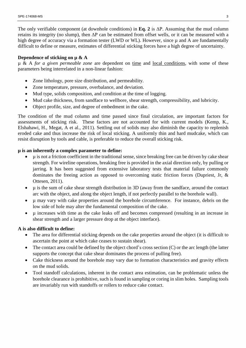
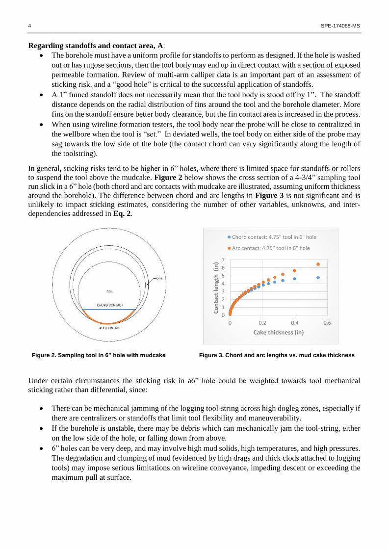
In general, sticking risks tend to be higher in 6” holes, where there is limited space for standoffs or rollers

to suspend the tool above the mudcake. Figure 2 below shows the cross section of a 4-3/4” sampling tool

run slick in a 6” hole (both chord and arc contacts with mudcake are illustrated, assuming uniform thickness

around the borehole). The difference between chord and arc lengths in Figure 3 is not significant and is

unlikely to impact sticking estimates, considering the number of other variables, unknowns, and inter-

dependencies addressed in Eq. 2.

Under certain circumstances the sticking risk in a6” hole could be weighted towards tool mechanical

sticking rather than differential, since:

There can be mechanical jamming of the logging tool-string across high dogleg zones, especially if

there are centralizers or standoffs that limit tool flexibility and maneuverability.

If the borehole is unstable, there may be debris which can mechanically jam the tool-string, either

on the low side of the hole, or falling down from above.

6” holes can be very deep, and may involve high mud solids, high temperatures, and high pressures.

The degradation and clumping of mud (evidenced by high drags and thick clods attached to logging

tools) may impose serious limitations on wireline conveyance, impeding descent or exceeding the

maximum pull at surface.

0

1

2

3

4

5

6

7

0 0.2 0.4 0.6

Co

nta

ct le

ngt

h (

in)

Cake thickness (in)

Chord contact: 4.75" tool in 6" hole

Arc contact: 4.75" tool in 6" hole

Figure 3. Chord and arc lengths vs. mud cake thickness

Figure 2. Sampling tool in 6” hole with mudcake

SPE-174068-MS 5

Dependency of sticking on station time

For cylindrical objects, such as drill pipe, logging tools, or cable, the pull-to-free force per unit length is

proportional to t 0.25 (Underhill, Moore, & Meeten, 1998; Reid, et al., 1996), where t = stationary time of

the object from the moment the toolstring stops on station (after which cake compression and extension

can compound the sticking forces). The result of this time dependency factor is that “a doubling of the

stationary time results in less than a 20% increase in sticking forces. Conversely, to cut the sticking risk in

half (without changing anything else), the stationary time must be reduced by 95%.” From an empirical

study of wireline sampling jobs with cable sticking (Kemp, K., Elshahawi, H., Megat, A. et al., 2011), it

was concluded that the main driver for cable sticking was time after drilling (hole/mud deterioration) and

not time on station.

In the formation sampling scenario, the clean-up times can typically vary from 30 – 300 minutes (generally

far down the t 0.25 graph). This fact suggests that the best approach to reduce sticking is:

To ensure the hole remains in good shape throughout the logging operation.

To minimize the contact area of all downhole logging equipment (tools and cable). If the mudcake

cannot find initial purchase on the downhole equipment, it cannot develop stronger sticking forces

later.

Cable sticking complexities

Cable sticking can be quite different from tool sticking for the following reasons:

Unlike logging tools which possess stiffness, logging cable is flexible, and can remain in full contact

with mudcake and formation around the bends in a wellbore.

Due to its small diameter, logging cable can apply high cutting thrusts against the mudcake and

formation, exposing deeper pressure imbalances which other logging equipment might not see.

Logging cable, which is generally elliptical ‘off the drum’, can deform under tension and pressure,

and may compound its contact area when under differential sticking forces.

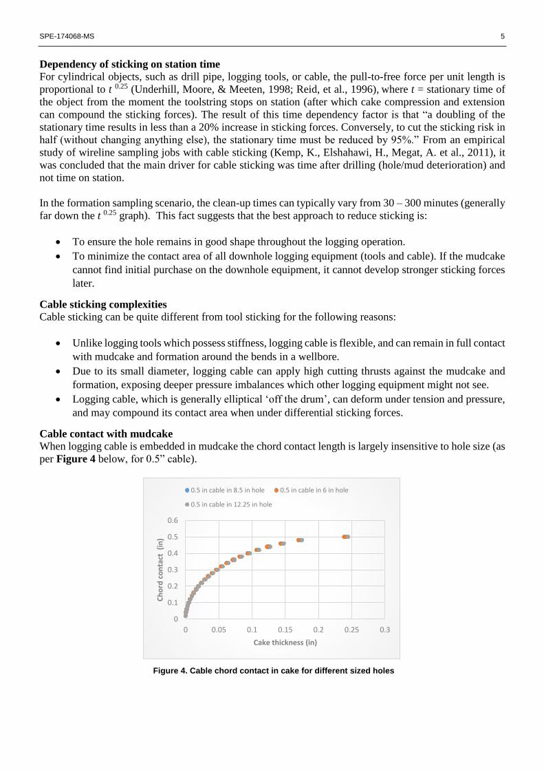
Cable contact with mudcake

When logging cable is embedded in mudcake the chord contact length is largely insensitive to hole size (as

per Figure 4 below, for 0.5” cable).

0

0.1

0.2

0.3

0.4

0.5

0.6

0 0.05 0.1 0.15 0.2 0.25 0.3

Ch

ord

co

nta

ct (

in)

Cake thickness (in)

0.5 in cable in 8.5 in hole 0.5 in cable in 6 in hole

0.5 in cable in 12.25 in hole

Figure 4. Cable chord contact in cake for different sized holes

6 SPE-174068-MS

A key parameter for cable sticking estimations is the contact length along the borehole. Since cable is

flexible, it can shift from side to side in a sinuous borehole. Based on this action, the contact area is a

unique function of the arrangement of doglegs and bends in the wellbore being logged.

In short, cable trajectory and contact lengths for differential sticking are difficult to ascertain. One

possibility is to combine ultrasonic borehole geometry data with downhole mud properties into a

sophisticated 3D cable force model. Currently, this is not a practical approach for field operations and the

necessary input data (e.g. variable mud properties) may be unavailable or inaccurate.

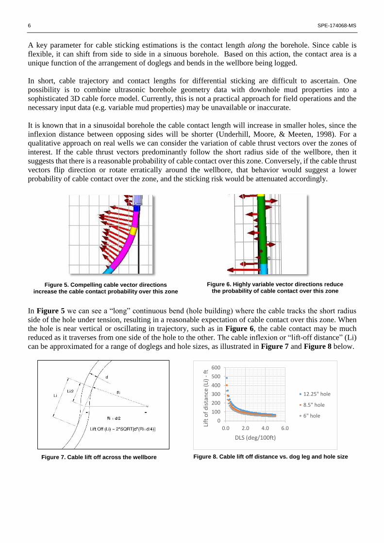
It is known that in a sinusoidal borehole the cable contact length will increase in smaller holes, since the

inflexion distance between opposing sides will be shorter (Underhill, Moore, & Meeten, 1998). For a

qualitative approach on real wells we can consider the variation of cable thrust vectors over the zones of

interest. If the cable thrust vectors predominantly follow the short radius side of the wellbore, then it

suggests that there is a reasonable probability of cable contact over this zone. Conversely, if the cable thrust

vectors flip direction or rotate erratically around the wellbore, that behavior would suggest a lower

probability of cable contact over the zone, and the sticking risk would be attenuated accordingly.

In Figure 5 we can see a “long” continuous bend (hole building) where the cable tracks the short radius

side of the hole under tension, resulting in a reasonable expectation of cable contact over this zone. When

the hole is near vertical or oscillating in trajectory, such as in Figure 6, the cable contact may be much

reduced as it traverses from one side of the hole to the other. The cable inflexion or “lift-off distance” (Li)

can be approximated for a range of doglegs and hole sizes, as illustrated in Figure 7 and Figure 8 below.

0

100

200

300

400

500

600

0.0 2.0 4.0 6.0

Lift

of

dis

tan

ce (

Li)

-ft

DLS (deg/100ft)

12.25" hole

8.5" hole

6" hole

Figure 5. Compelling cable vector directions increase the cable contact probability over this zone

Figure 6. Highly variable vector directions reduce the probability of cable contact over this zone

Figure 7. Cable lift off across the wellbore

Figure 8. Cable lift off distance vs. dog leg and hole size

SPE-174068-MS 7

Ultimately, it is the linkage of doglegs and cable forces that define cable contact in a wellbore. Figure 8

demonstrates that cable inflexion may result in no contact with formation for ≈ 80 to 180 ft. over a common

range of doglegs (0.5 to 2.5 deg/100ft in 8-1/2” hole), considerably reducing the risk of cable sticking risk

over this zone. The detailed analysis of the hole trajectory, and possible inflexions over the zones of interest

(including from above and below), are important factors in the overall cable sticking risk assessment.

In all cases, what truly matters is the cable’s physical contact with mudcake on a macro level in the

wellbore. True cable contact is a function of tension, trajectory, micro-doglegs, rugosity, and distribution

of mudcake thicknesses in the wellbore. In practical terms, the static drilling survey may not yield sufficient

information to create an accurate borehole geometry model. High resolution wireline data or continuous

MWD data would be needed for that. Petrophysical measurements would also be needed to detect the

presence (and ideally the thicknesses) of mudcake distributions around and along the wellbore.

Cable keyseating

Keyseating is term originating from drilling operations where a “key hole” profile is worn into the wellbore

by the drill pipe body that subsequently catches the pipe joint (of larger diameter) when attempting to pull

out of hole. A similar phenomenon can occur with wireline cable, where it cuts a groove in a soft formation

(or a ledge), causing the logging cable head to be caught as the tools are pulled out of the hole. The

propensity for a cable to cut a groove into formation was determined to be a function of cable tension (T),

dogleg (Ө𝑑), contact length (L), and cable diameter (dc) (Underhill, Moore, & Meeten, 1998), as per Eq. 3

below:

𝐶𝑢𝑡𝑡𝑖𝑛𝑔 𝑠𝑡𝑟𝑒𝑠𝑠 𝑡𝑜 𝑓𝑜𝑟𝑚𝑎𝑡𝑖𝑜𝑛 = 𝑇Ө𝑑

𝐿𝑑𝑐…………………………(Eq.3)

The other factor which will influence keyseating (other things being equal) is the duration that the cutting

stress is applied. For instance, the quantity of tensioned cable that passes through the keyseating zones will

increase the possibility of keyseating. This situation is often found in formation testers, which may involve

a high number of cable cycles during a pressure survey. This thinking implies that heavy tool strings in

deep and deviated sections may result in a higher keyseating risk.

In certain cases, the wireline may rotate in the keyseating groove (from cable torque), which could aid the

excavation of mudcake. If the lateral thrust is high, then cable rotation may cease, but the helical nature of

the armor (analogous to a twist drill) may still assist with groove extension as cable is pulled through the

keyseating zone.

The contact mechanics of logging cable with formation are complicated since:

Both cable and formation are elastic and may deform under pressure.

The pressure applied by the cable may result from tension around a dogleg or from differential

pressure across the cable (or both, the driver of drag may change as the U-groove deepens).

Rock mechanical effects on groove excavation and sticking are unknown.

Mud lubrication effects on groove excavation and sticking are unknown.

Cable torsion effects on groove excavation and sticking are unknown.

Solids entrainment (or ejection) on groove excavation and sticking are unknown.

8 SPE-174068-MS

Bearing these complexities in mind, a simple risk assessment for wireline keyseating can be made by asking

the following questions:

What are the formation lithologies and strengths in the deviated and high dogleg zones?

What are the modeled cable thrusts positioned high in these zones?

How much tensioned wireline cable will pass through these zones? (lbs./ft?)

An alternative interpretation of cable keyseating does not concern catching the logging head in a ‘U’

groove. Rather it is when the cumulative cable drag in a tortuous well raises the surface tension to the limit

of the logging package.

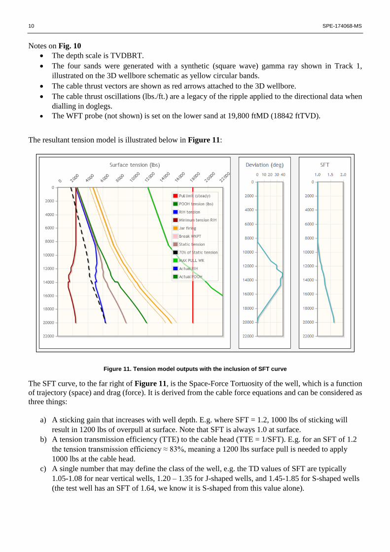
When a logging cable cuts a deep ‘U’ groove in a formation, a drag hot-spot may be formed, exacerbated

by differential sticking forces across the groove, if present (compressing the cable and creating additional

wall thrust). It should be noted that wireline sheaves are designed to cradle between 120º and 150º of the

cable diameter to avoid pinching. “Keyseating drag” can be analogous to running a belt that is too large

for its pulley. Differing degrees of keyseating in a permeable formation are illustrated below in Figure 9.

Figure 9. Cable keyseating with differential sticking

The impact of wireline cable keyseating varies according to formation and cable penetration:

Cutting through cake may only induce differential sticking forces.

Cutting through cake and formation may increase those differential sticking forces.

Cutting deep ‘U’ grooves may create drag hot spots, resulting in differential sticking and radial

thrust via cable deformation.

Keyseating may be intimately linked with cable differential sticking in deviated wellbores, but estimating

(or verifying) the effects of cable U-grooves on surface tension is very difficult to do. This subject is not

covered in this paper. Rock mechanics and mud interaction are also very interesting areas for future

investigation. Determining whether formation stresses and/or mud reactions may result in groove

contraction on the cable is a subject worthy of additional study.

Effect of cable sticking on surface tension

Cable force equations for wireline tension models have been explained at length in other papers and will

not be repeated here (McSpadden, Brown, & Davis, 2001; Johancsik, Frieson, & Dawson, 1983). In this

paper, we will describe the principles of an enhanced tension model that incorporates differential sticking

forces for tools and cable.

Cable cutting through cake, leading

to differential sticking forces

Cable cutting into formation with

more cable area exposed to

differential sticking forces

Cable cutting deeper into the formation.

Differential sticking, cable deformation,

and side wall thrust (drag) may be

maximized

SPE-174068-MS 9

The sticking forces are evaluated in four stages:

1) Inclusion of wellbore gamma data (synthetic or real) for the initial estimate of permeable zones per

cable element in the tension model.

2) Estimation of differential sticking forces per cable element, based on the overbalance, contact area,

and assigned sticking coefficient (Eq. 2).

3) Integration of sticking forces to the tension model (tools or cable) projected up to the surface.

4) Refinement of the potential sticking zones by the addition of petrophysical data, such as continuous

NMR, or other logs that indicate the presence of permeable zones with sticking potential.

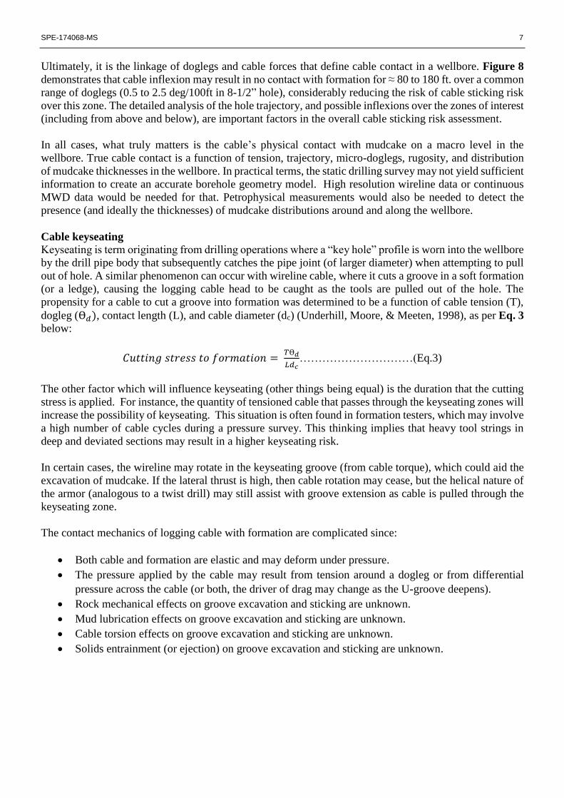
To best explain the concept of the model we will examine a theoretical test well, 20 Kft deep, with four

evenly distributed sticky sands, the lowest of which will be sampled with a Wireline Formation Tester

(WFT). The basic well details are highlighted in Table 1. The sticking coefficient, µ, has been set to 0.05

(without any time dependence), a rough estimate only, commonly available from mud manuals.

TEST WELL FOR STICKING ANALYSIS

Total depth (TD) - 8 -1/2” 20,000 ft MD)

Mud type OBM

Casing shoe – 9-5/8” 14,000 ft (MD) Mud weight 10.0 ppg

WFT weight in air & length 3,600 lbs/110 ft Uniform overbalance 1.0 ppg

Nominal jar trigger 4,500 lbs (+/- 10%) ΔSFT range over 4 sands 1.34 - 1.63

Number of sticking sands (n) 4 x 100 ft (MD) Maximum SFT (at TD) 1.64

Sticking coefficient 0.05 Maximum pull at surface 18,000 lbs

Table 1. Details of S-shaped test well for sticking analysis

Figure 10. Test well lower section illustrating the four key sands and cable thrust vectors

10 SPE-174068-MS

Notes on Fig. 10

The depth scale is TVDBRT.

The four sands were generated with a synthetic (square wave) gamma ray shown in Track 1,

illustrated on the 3D wellbore schematic as yellow circular bands.

The cable thrust vectors are shown as red arrows attached to the 3D wellbore.

The cable thrust oscillations (lbs./ft.) are a legacy of the ripple applied to the directional data when

dialling in doglegs.

The WFT probe (not shown) is set on the lower sand at 19,800 ftMD (18842 ftTVD).

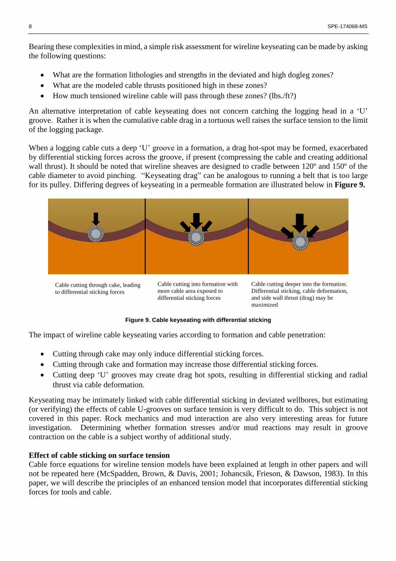
The resultant tension model is illustrated below in Figure 11:

Figure 11. Tension model outputs with the inclusion of SFT curve

The SFT curve, to the far right of Figure 11, is the Space-Force Tortuosity of the well, which is a function

of trajectory (space) and drag (force). It is derived from the cable force equations and can be considered as

three things:

a) A sticking gain that increases with well depth. E.g. where SFT = 1.2, 1000 lbs of sticking will

result in 1200 lbs of overpull at surface. Note that SFT is always 1.0 at surface.

b) A tension transmission efficiency (TTE) to the cable head (TTE = 1/SFT). E.g. for an SFT of 1.2

the tension transmission efficiency ≈ 83%, meaning a 1200 lbs surface pull is needed to apply

1000 lbs at the cable head.

c) A single number that may define the class of the well, e.g. the TD values of SFT are typically

1.05-1.08 for near vertical wells, 1.20 – 1.35 for J-shaped wells, and 1.45-1.85 for S-shaped wells

(the test well has an SFT of 1.64, we know it is S-shaped from this value alone).

SPE-174068-MS 11

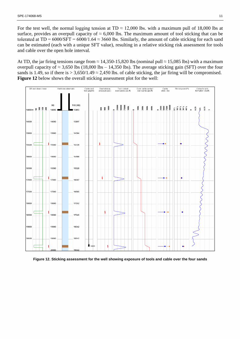
For the test well, the normal logging tension at TD ≈ 12,000 lbs. with a maximum pull of 18,000 lbs at

surface, provides an overpull capacity of ≈ 6,000 lbs. The maximum amount of tool sticking that can be

tolerated at TD = 6000/SFT = 6000/1.64 ≈ 3660 lbs. Similarly, the amount of cable sticking for each sand

can be estimated (each with a unique SFT value), resulting in a relative sticking risk assessment for tools

and cable over the open hole interval.

At TD, the jar firing tensions range from ≈ 14,350-15,820 lbs (nominal pull ≈ 15,085 lbs) with a maximum

overpull capacity of ≈ 3,650 lbs (18,000 lbs – 14,350 lbs). The average sticking gain (SFT) over the four

sands is 1.49, so if there is > 3,650/1.49 ≈ 2,450 lbs. of cable sticking, the jar firing will be compromised.

Figure 12 below shows the overall sticking assessment plot for the well:

Figure 12. Sticking assessment for the well showing exposure of tools and cable over the four sands

12 SPE-174068-MS

Notes on Fig. 12:

Track 1 is the synthetic gamma ray curve, with clean sands illustrated as red bars.

Track 2 is the wellbore schematic with the clean sands illustrated as brown blocks.

Track 3 shows the positions of tool, probe, and cable in the wellbore (to scale).

Track 4 is the overbalance in psi (a uniform 1 ppg has been applied for this well).

Track 5 is the tool psi.ft plot assuming the larger diameter WFT is 85 ft. long, with 15 ft. of normal

sized tools connected above (jars and telemetry cartridge, which are fully suspended by standoffs

and not included in the sticking assessment).

Track 6 is the cumulative cable psi.ft., which shows step changes as each clean sand is encountered.

Track 7 is the sand sticking plot: blue is downhole sticking (lbs.); orange is the overpull at surface

(lbs).

Track 8 is the sand relative sticking %: blue is downhole sticking; orange is the overpull at surface.

Track 9 is the cable thrust, also shown in Figure 10.

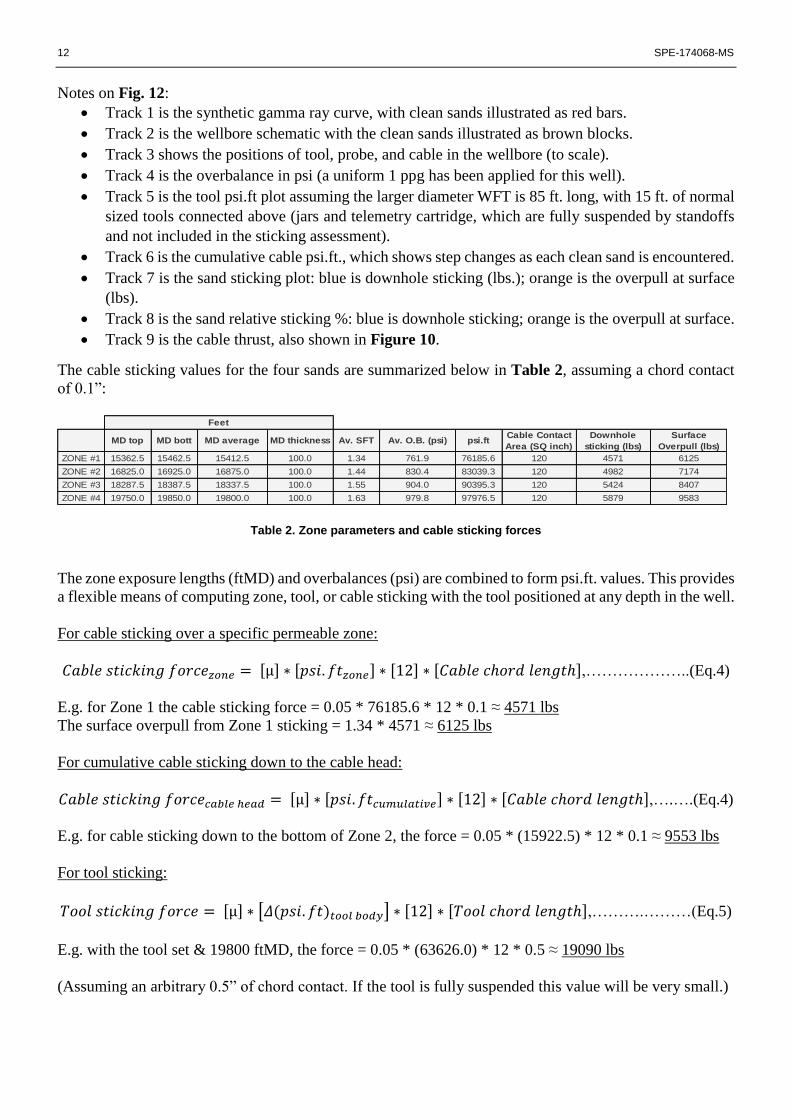
The cable sticking values for the four sands are summarized below in Table 2, assuming a chord contact

of 0.1”:

MD top MD bott MD average MD thickness Av. SFT Av. O.B. (psi) psi.ftCable Contact

Area (SQ inch)

Downhole

sticking (lbs)

Surface

Overpull (lbs)

ZONE #1 15362.5 15462.5 15412.5 100.0 1.34 761.9 76185.6 120 4571 6125

ZONE #2 16825.0 16925.0 16875.0 100.0 1.44 830.4 83039.3 120 4982 7174

ZONE #3 18287.5 18387.5 18337.5 100.0 1.55 904.0 90395.3 120 5424 8407

ZONE #4 19750.0 19850.0 19800.0 100.0 1.63 979.8 97976.5 120 5879 9583

Feet

Table 2. Zone parameters and cable sticking forces

The zone exposure lengths (ftMD) and overbalances (psi) are combined to form psi.ft. values. This provides

a flexible means of computing zone, tool, or cable sticking with the tool positioned at any depth in the well.

For cable sticking over a specific permeable zone:

𝐶𝑎𝑏𝑙𝑒 𝑠𝑡𝑖𝑐𝑘𝑖𝑛𝑔 𝑓𝑜𝑟𝑐𝑒𝑧𝑜𝑛𝑒 = [µ] ∗ [𝑝𝑠𝑖. 𝑓𝑡𝑧𝑜𝑛𝑒] ∗ [12] ∗ [𝐶𝑎𝑏𝑙𝑒 𝑐ℎ𝑜𝑟𝑑 𝑙𝑒𝑛𝑔𝑡ℎ],………………..(Eq.4)

E.g. for Zone 1 the cable sticking force = 0.05 * 76185.6 * 12 * 0.1 ≈ 4571 lbs

The surface overpull from Zone 1 sticking = 1.34 * 4571 ≈ 6125 lbs

For cumulative cable sticking down to the cable head:

𝐶𝑎𝑏𝑙𝑒 𝑠𝑡𝑖𝑐𝑘𝑖𝑛𝑔 𝑓𝑜𝑟𝑐𝑒𝑐𝑎𝑏𝑙𝑒 ℎ𝑒𝑎𝑑 = [µ] ∗ [𝑝𝑠𝑖. 𝑓𝑡𝑐𝑢𝑚𝑢𝑙𝑎𝑡𝑖𝑣𝑒] ∗ [12] ∗ [𝐶𝑎𝑏𝑙𝑒 𝑐ℎ𝑜𝑟𝑑 𝑙𝑒𝑛𝑔𝑡ℎ],….….(Eq.4)

E.g. for cable sticking down to the bottom of Zone 2, the force = 0.05 * (15922.5) * 12 * 0.1 ≈ 9553 lbs

For tool sticking:

𝑇𝑜𝑜𝑙 𝑠𝑡𝑖𝑐𝑘𝑖𝑛𝑔 𝑓𝑜𝑟𝑐𝑒 = [µ] ∗ [𝛥(𝑝𝑠𝑖. 𝑓𝑡)𝑡𝑜𝑜𝑙 𝑏𝑜𝑑𝑦] ∗ [12] ∗ [𝑇𝑜𝑜𝑙 𝑐ℎ𝑜𝑟𝑑 𝑙𝑒𝑛𝑔𝑡ℎ],……….………(Eq.5)

E.g. with the tool set & 19800 ftMD, the force = 0.05 * (63626.0) * 12 * 0.5 ≈ 19090 lbs

(Assuming an arbitrary 0.5” of chord contact. If the tool is fully suspended this value will be very small.)

SPE-174068-MS 13

For cable element sticking (in the tension model):

𝐶𝑎𝑏𝑙𝑒 𝑠𝑡𝑖𝑐𝑘𝑖𝑛𝑔 𝑓𝑜𝑟𝑐𝑒𝑒𝑙𝑒𝑚𝑒𝑛𝑡 = [µ] ∗ [𝑝𝑠𝑖. 𝑓𝑡𝑒𝑙𝑒𝑚𝑒𝑛𝑡] ∗ [12] ∗ [𝐶𝑎𝑏𝑙𝑒 𝑐ℎ𝑜𝑟𝑑 𝑙𝑒𝑛𝑔𝑡ℎ],……..……(Eq.6)

The Total Downhole Sticking (TDS), from n sticky sands is additive, as below:

𝑇𝐷𝑆 (𝑙𝑏𝑠) = ∑ [µ ∗ [𝑝𝑠𝑖. 𝑓𝑡𝑖] ∗ [12] ∗ [𝑐ℎ𝑜𝑟𝑑 𝑙𝑒𝑛𝑔𝑡ℎ]]𝑛𝑖=1 ,………………………........………….(Eq.7)

The Total Surface Overpull (TSO) employs the sticking gains (SFTs) for each zone:

𝑇𝑆𝑂 (𝑙𝑏𝑠) = ∑ [µ ∗ [𝑝𝑠𝑖. 𝑓𝑡𝑖] ∗ [12] ∗ [𝑐ℎ𝑜𝑟𝑑 𝑙𝑒𝑛𝑔𝑡ℎ] ∗ 𝑆𝐹𝑇𝑖]𝑛𝑖=1 ,…………………...........…..…(Eq.8)

∴ If TSO exceeds the limit of the logging package, then the wireline equipment may be declared stuck.

Note that the cable chord limit (leading to a cable contact limit to reach maximum pull) can also be

determined, as below:

𝐶𝑎𝑏𝑙𝑒 𝑐ℎ𝑜𝑟𝑑 𝑙𝑖𝑚𝑖𝑡 = 𝑀𝑎𝑥 𝑜𝑣𝑒𝑟𝑝𝑢𝑙𝑙 𝑐𝑎𝑝𝑎𝑐𝑖𝑡𝑦

∑ [µ]∗[12]∗[𝑝𝑠𝑖.𝑓𝑡𝑖]∗ [𝑆𝐹𝑇𝑖]𝑛𝑖=1

,……………………………………........................(Eq.9)

With the tool sampling in Zone 4 @ 19800 ftMD we can estimate the cable chord contact over the upper

three sands (300 ft. in measured length) to result in the surface overpull limit of 6000 lbs:

𝐶𝑎𝑏𝑙𝑒 𝑐ℎ𝑜𝑟𝑑 𝑙𝑖𝑚𝑖𝑡 = 6000

[0.05 ∗ 12 ∗ [76185.6 ∗ 1.34 + 83039.3 ∗ 1.44 + 90395.3 ∗ 1.55]= 0.028"

𝐶𝑎𝑏𝑙𝑒 𝑐𝑜𝑛𝑡𝑎𝑐𝑡 𝑎𝑟𝑒𝑎𝑙𝑖𝑚𝑖𝑡 = 𝐶𝑎𝑏𝑙𝑒 𝑐ℎ𝑜𝑟𝑑 𝑙𝑖𝑚𝑖𝑡 ∗ 𝐶𝑜𝑛𝑡𝑎𝑐𝑡 𝑙𝑒𝑛𝑔𝑡ℎ (𝑖𝑛)

𝐶𝑎𝑏𝑙𝑒 𝑐𝑜𝑛𝑡𝑎𝑐𝑡 𝑎𝑟𝑒𝑎𝑙𝑖𝑚𝑖𝑡 = 0.028 ∗ 300 𝑥 12 ≈ 100 𝑖𝑛2

For arguments sake, if we assume a uniform 1/8” mud cake thickness over the 300 ft. of upper sands, then

the cable chord contact is ≈ 0.43” for a 0.5” cable, as per Figure 4.

In which case, the necessary cable contact along the borehole to generate this level of sticking ≈ 100/0.43

≈ 234 inches ≈ 19.5 ft.

Thus, we can say that if ≈ 20 ft. of cable is embedded in 1/8” cake over the upper three sands, the cable

may become stuck. 18,000 lbs. surface tension could be generated by less than 10% of contact and sticking

(20ft/300ft). In this case, it would be recommended to deploy WLSOs over these upper sands.

In this example we have assumed a nominal cable chord contact of 0.1”. This value is adjusted during the

modeling to explore the net effect on surface overpull. Also, the sticking coefficient µ was set to 0.05 (for

OBM, at time t=t0). Since µ increases with time, this nominal value would produce the minimal sticking

forces (other things being equal).

14 SPE-174068-MS

From Eq.8, we can see there can be an infinite number of sticking combinations to reach maximum pull at

surface. The sticking risk varies with:

a. The overpull capacity at surface (“Max” pull minus the normal logging tension or jar firing tension).

b. The number of exposed permeable sands (n).

c. The overbalance and extent of the exposed permeable sands (psi.ft.).

d. The cable contact area over the exposed permeable sands (fn chord length).

e. The SFT of the exposed permeable sands, and also the change in SFT (ΔSFT) over those sands.

For example, if an S-shaped well is being logged on land in a WBM environment, the overall sticking risk

might be considered high since:

a) The truck may have limited overpull capacity (high tension logging packages are rare on land jobs).

b) The SFT may be 1.5-1.8, amplifying the sticking forces considerably, and quickly consuming the

overpull capacity.

c) The sticking coefficient for WBM is generally higher than for OBM.

Two other important factors for assessing cable sticking risk are:

a) Cable thrust over the exposed permeable sands, which may excavate the cake, reveal the pressure

imbalance, and induce differential sticking forces. The level of thrust is directly related to the ΔSFT

over the open hole interval.

b) The number of cable cycles over the exposed permeable sands, creating a cutting action that can

penetrate deeper into the cake and exacerbate the differential sticking forces.

Conclusions about cable sticking from this study:

Space-force tortuosity (SFT) is an amplifier of downhole sticking forces (for cable or tools). The

deeper and more tortuous the sticking zone, the higher the overall contribution to surface pull.

A higher ΔSFT in the open hole implies significant directional changes and associated cable thrusts,

which may increase the cable sticking risk (in this well it ranges from 1.27 at the casing shoe to

1.64 at TD).

Tool and cable sticking forces can combine together in an infinite number of ways to exceed

maximum pull at surface. The relative sticking percentage depends on the location of the sticking

zones (SFTs), along with the tool and cable contact areas.

The higher the jar trigger, the less overpull capacity there is to overcome cable sticking, and the

higher the risk in not being able to fire or re-cock the jar.

True cable contact (and sticking potential) is difficult to know with confidence, but a qualitative

approach is useful to assess the broad sticking sensitivity of the well. In this case < 20 ft. of cable

sticking (in 1/8” mudcake) from 300 ft. of exposed sands (< 10% of gross sands) may result in the

need for a fishing job. Similarly, < 12 ft. of cable contact may impede jar firing.

SPE-174068-MS 15

Real well environment and sticking assessment

From Eq.9 there is not so much the logging provider can do to influence the wellbore environment prior to

rigging up, since:

The overall wellbore trajectory (SFT) has been determined by the objectives,

constraints, and risks facing the Operator (technical, geographic, and economic).

For any given logging package the higher the SFT, the less the capacity for

overpull. Moreover, the higher the ΔSFT across the open-hole section, the higher

the sticking risks when cable thrusts are aligned with cake bearing zones.

The overbalance (psi) and permeable zones (ft.) are governed by the well design

and drilling tolerance window.

The sticking coefficient, µ, is not generally a parameter employed in the mud

recipe (or included in the daily mud report for review or adjustment).

For formation sampling operations, the time on station is usually defined by the

sample contamination goal (%). Thus the time dependent sticking properties (µ,

and A) are not really controllable by the logging crew (although optimized pump

and probe selection can certainly help minimize the time on station).

Equipment contact reduction to mitigate sticking

Aside from conducting a detailed wireline risk assessment, and arranging for the

best logging equipment to be available (hoist, cable, release head, and jars) the

logging provider is restricted to two main areas for differential sticking mitigation:

a) Maintaining vigilance on hole conditions throughout the logging operation, and

requesting a wiper trip if the hole has been open for a long time, or is showing

signs of deterioration.

b) Reducing the contact area and drag of all downhole logging equipment (tools

and cable).

There has been solid progress to reduce logging tool contact, the deployment of low area standoffs and

roller assemblies being a key development (Prasad, Castillo, & Elshahawi, 2012). However, the cable can

remain highly vulnerable to sticking unless it can be suspended from the mudcake and formation in a similar

fashion. Therefore, there is motivation to develop the wireline standoff (WLSO).

Wireline Standoff (WLSO) to reduce cable contact area

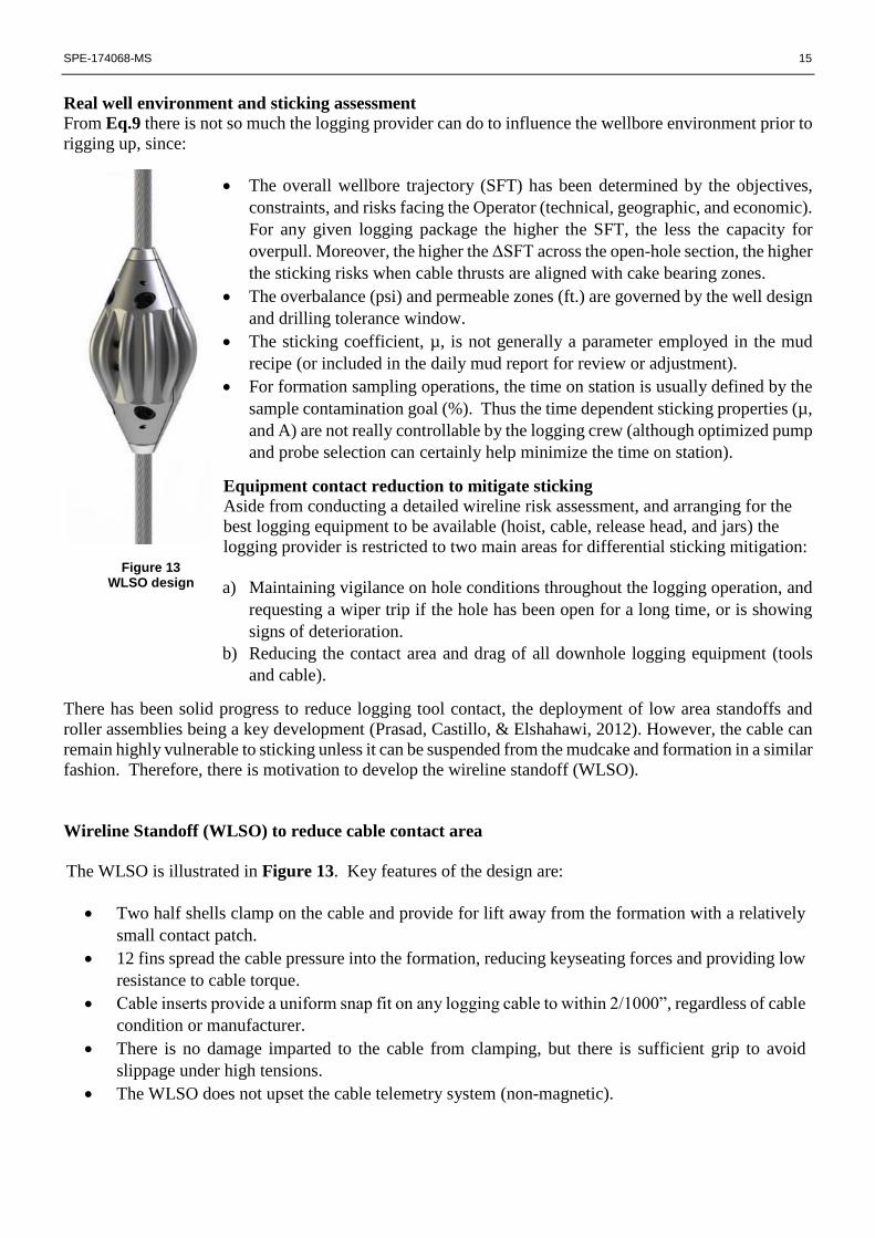
The WLSO is illustrated in Figure 13. Key features of the design are:

Two half shells clamp on the cable and provide for lift away from the formation with a relatively

small contact patch.

12 fins spread the cable pressure into the formation, reducing keyseating forces and providing low

resistance to cable torque.

Cable inserts provide a uniform snap fit on any logging cable to within 2/1000”, regardless of cable

condition or manufacturer.

There is no damage imparted to the cable from clamping, but there is sufficient grip to avoid

slippage under high tensions.

The WLSO does not upset the cable telemetry system (non-magnetic).

Figure 13 WLSO design

16 SPE-174068-MS

The standard WLSO diameter of 2.95” allows stripping over using a 3-3/8” grapple during fishing

operations.

A low angle of attack and a streamline profile that avoids hang up points in the wellbore such as

the casing shoe.

Use of lanyards to avoid dropped object risks during installation and removal on the cable.

A durable body, enhanced with laser hard coating, to resist fin wear in casing and hard formation.

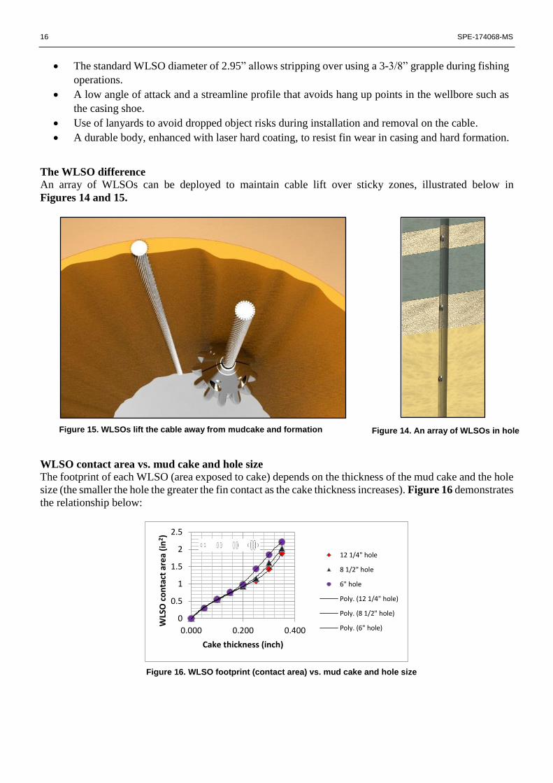
The WLSO difference

An array of WLSOs can be deployed to maintain cable lift over sticky zones, illustrated below in

Figures 14 and 15.

WLSO contact area vs. mud cake and hole size

The footprint of each WLSO (area exposed to cake) depends on the thickness of the mud cake and the hole

size (the smaller the hole the greater the fin contact as the cake thickness increases). Figure 16 demonstrates

the relationship below:

0

0.5

1

1.5

2

2.5

0.000 0.200 0.400

WLS

O c

on

tact

are

a (i

n2 )

Cake thickness (inch)

12 1/4" hole

8 1/2" hole

6" hole

Poly. (12 1/4" hole)

Poly. (8 1/2" hole)

Poly. (6" hole)

Figure 15. WLSOs lift the cable away from mudcake and formation Figure 14. An array of WLSOs in hole

Figure 16. WLSO footprint (contact area) vs. mud cake and hole size

SPE-174068-MS 17

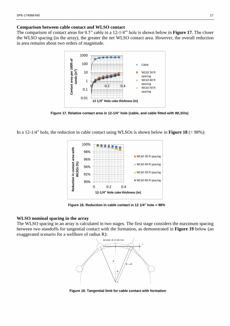
Comparison between cable contact and WLSO contact

The comparison of contact areas for 0.5” cable in a 12-1/4'” hole is shown below in Figure 17. The closer

the WLSO spacing (in the array), the greater the net WLSO contact area. However, the overall reduction

in area remains about two orders of magnitude.

In a 12-1/4” hole, the reduction in cable contact using WLSOs is shown below in Figure 18 (> 98%):

WLSO nominal spacing in the array

The WLSO spacing in an array is calculated in two stages. The first stage considers the maximum spacing

between two standoffs for tangential contact with the formation, as demonstrated in Figure 19 below (an

exaggerated scenario for a wellbore of radius R):

0.01

0.1

1

10

100

1000

0 0.2 0.4

Co

nta

ct a

rea

pe

r 1

00

ft o

f sa

nd

s (i

n2 )

12 1/4" Hole cake thickness (in)

Cable

WLSO 30 ftspacingWLSO 40 ftspacingWLSO 50 ftspacing

90%

92%

94%

96%

98%

100%

0 0.2 0.4

Re

du

ctio

n in

co

nta

ct a

rea

wit

h

WLS

Os

(%)

12-1/4" Hole cake thickness (in)

WLSO 30 ft spacing

WLSO 40 ft spacing

WLSO 50 ft spacing

WLSO 60 ft spacing

Figure 17. Relative contact area in 12-1/4" hole (cable, and cable fitted with WLSOs)

Figure 18. Reduction in cable contact in 12 1/4" hole > 98%

Figure 19. Tangential limit for cable contact with formation

18 SPE-174068-MS

For the tangential condition:

Cos(Ө) =R+r

R+dR ; WLSO spacing = 2 ∗ (R + dR) ∗ Sin(Ө),………………………………………………….(Eq.10)

Where: R =100

Radians (DLS) ; dR = WLSO radius; r = cable radius

The resulting crossplot for WLSO spacing vs. DLS is shown below in Figure 20:

Cable sag

Cable sag (drooping) between standoffs, or between adjacent arrays on the cable, must be included in the

WLSO job plan to ensure there will be no cable contact with formation or mud cake. For small sag-to-span

ratios (as with a wireline cable under normal logging tensions), the sagging cable curve can be described

by a parabolic equation, which provides very close results to that gained by the traditional catenary

equation. Details of the sag equations are shown in Appendix A-1.

Example WLSO job – Gulf of Mexico

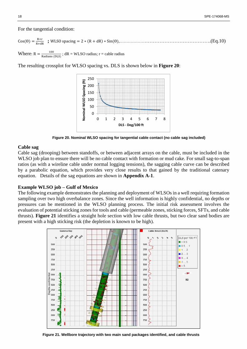
The following example demonstrates the planning and deployment of WLSOs in a well requiring formation

sampling over two high overbalance zones. Since the well information is highly confidential, no depths or

pressures can be mentioned in the WLSO planning process. The initial risk assessment involves the

evaluation of potential sticking zones for tools and cable (permeable zones, sticking forces, SFTs, and cable

thrusts). Figure 21 identifies a straight hole section with low cable thrusts, but two clear sand bodies are

present with a high sticking risk (the depletion is known to be high).

0

50

100

150

200

250

0 1 2 3 4 5 6 7 8No

min

al W

LSO

Sp

acin

g (f

t)

DLS - Deg/100 ft

Figure 21. Wellbore trajectory with two main sand packages identified, and cable thrusts

Figure 20. Nominal WLSO spacing for tangential cable contact (no cable sag included)

SPE-174068-MS 19

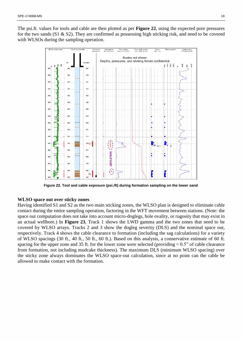
The psi.ft. values for tools and cable are then plotted as per Figure 22, using the expected pore pressures

for the two sands (S1 & S2). They are confirmed as possessing high sticking risk, and need to be covered

with WLSOs during the sampling operation.

WLSO space out over sticky zones

Having identified S1 and S2 as the two main sticking zones, the WLSO plan is designed to eliminate cable

contact during the entire sampling operation, factoring in the WFT movement between stations. (Note: the

space out computation does not take into account micro-doglegs, hole ovality, or rugosity that may exist in

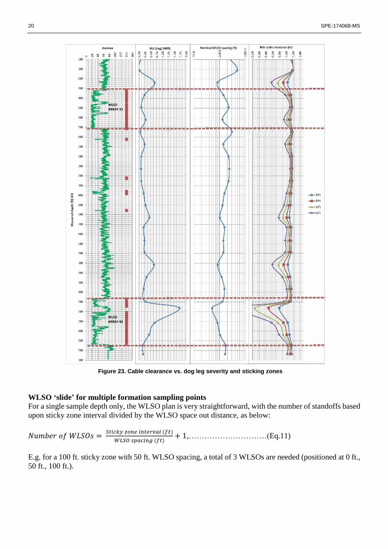
an actual wellbore.) In Figure 23, Track 1 shows the LWD gamma and the two zones that need to be

covered by WLSO arrays. Tracks 2 and 3 show the dogleg severity (DLS) and the nominal space out,

respectively. Track 4 shows the cable clearance to formation (including the sag calculations) for a variety

of WLSO spacings (30 ft., 40 ft., 50 ft., 60 ft.). Based on this analysis, a conservative estimate of 60 ft.

spacing for the upper zone and 35 ft. for the lower zone were selected (providing ≈ 0.5” of cable clearance

from formation, not including mudcake thickness). The maximum DLS (minimum WLSO spacing) over

the sticky zone always dominates the WLSO space-out calculation, since at no point can the cable be

allowed to make contact with the formation.

Figure 22. Tool and cable exposure (psi./ft) during formation sampling on the lower sand

20 SPE-174068-MS

WLSO ‘slide’ for multiple formation sampling points

For a single sample depth only, the WLSO plan is very straightforward, with the number of standoffs based

upon sticky zone interval divided by the WLSO space out distance, as below:

𝑁𝑢𝑚𝑏𝑒𝑟 𝑜𝑓 𝑊𝐿𝑆𝑂𝑠 = 𝑆𝑡𝑖𝑐𝑘𝑦 𝑧𝑜𝑛𝑒 𝑖𝑛𝑡𝑒𝑟𝑣𝑎𝑙 (𝑓𝑡)

𝑊𝐿𝑆𝑂 𝑠𝑝𝑎𝑐𝑖𝑛𝑔 (𝑓𝑡)+ 1,…………………………(Eq.11)

E.g. for a 100 ft. sticky zone with 50 ft. WLSO spacing, a total of 3 WLSOs are needed (positioned at 0 ft.,

50 ft., 100 ft.).

Figure 23. Cable clearance vs. dog leg severity and sticking zones

SPE-174068-MS 21

When a series of formation samples are needed (as is usually the case) the WLSO plan has to include ‘slide’

calculations which bring new WLSOs into the sticky zones as the tool moves down from the upper to the

lower sample stations. This increases the number of WLSOs needed for the job, as below:

𝑁𝑢𝑚𝑏𝑒𝑟 𝑜𝑓 𝑊𝐿𝑆𝑂𝑠 = 𝑆𝑡𝑖𝑐𝑘𝑦 𝑧𝑜𝑛𝑒 𝑖𝑛𝑡𝑒𝑟𝑣𝑎𝑙 (𝑓𝑡)+𝑆𝑎𝑚𝑝𝑙𝑖𝑛𝑔 𝑠𝑝𝑎𝑛 (𝑓𝑡)

𝑊𝐿𝑆𝑂 𝑠𝑝𝑎𝑐𝑖𝑛𝑔 (𝑓𝑡)+ 1,……………………(Eq.12)

Thus, for a 100 ft. sticky zone with 50 ft. spacing of WLSOs and 100 ft. between upper and lower sample

stations, the number of WLSOs needed is 5 (when the tool moves down to the lower sample station, the

upper two WLSOs move down to protect the cable over the sticky zone).

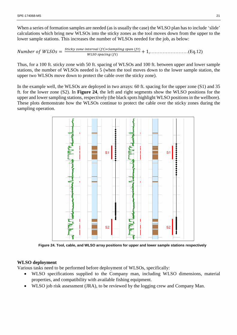
In the example well, the WLSOs are deployed in two arrays: 60 ft. spacing for the upper zone (S1) and 35

ft. for the lower zone (S2). In Figure 24, the left and right segments show the WLSO positions for the

upper and lower sampling stations, respectively (the black spots highlight WLSO positions in the wellbore).

These plots demonstrate how the WLSOs continue to protect the cable over the sticky zones during the

sampling operation.

WLSO deployment

Various tasks need to be performed before deployment of WLSOs, specifically:

WLSO specifications supplied to the Company man, including WLSO dimensions, material

properties, and compatibility with available fishing equipment.

WLSO job risk assessment (JRA), to be reviewed by the logging crew and Company Man.

Figure 24. Tool, cable, and WLSO array positions for upper and lower sample stations respectively

22 SPE-174068-MS

Cable size evaluation for WLSO insert selection, either from reviewing the cable shop maintenance

report (tabulated X-Y dimensions every 1000 ft.) or by digital calliper measurements on the drill

floor from an earlier logging run (with the cable under tension).

Installation of cable inserts, and the winchman stop depth sheet, generated from the WLSO plan.

Once the WLSO plan has been agreed upon, the hardware is moved to the drill floor. After making up the

wireline toolstring, the winchman stops at the first WLSO depth and the make-up plate is attached to the

cable with a clamp. A chain depth gauge ensures consistent positioning of WLSOs above the drill floor,

relative to tool zero (Figure 25). The first WLSO is then lifted with lanyards into the tapered bushing in

the make-up plate (Figure 26), and 4 new bolts are installed with a speed wrench. Final torque is applied

with a calibrated torque wrench (no grease on the threads). The installation time for a single WLSO is

approximately 2.5 – 3.0 minutes, and removal is < 1 minute. The winchman then proceeds to the next

WLSO stop depth, and the process is repeated. When all WLSOs are installed, the winchman proceeds in

hole as per standard operating procedures. When pulling out of hole, the upper WLSO depth is carefully

monitored at all times (into the casing shoe, past the BOPs, and approaching surface). At surface the

removal depths are also carefully recorded.

WLSO results and conclusions To date, 16 arrays of WLSOs have been successfully deployed on 8 wells to facilitate deep formation

sampling without incurring cable sticking. The average number of WLSOs per run ≈ 20 at 45 ft. spacing

(the minimum number of WLSOs deployed = 5; the maximum = 34). On one occasion, modest overpulls

were observed coming off station, which was attributed to WLSO sticking in ultra-high overbalance zones

(the estimated contact area per WLSO ≈ 0.5 in2).

A set of WLSO planning models have been developed which:

Can identify wells in which general sticking risk is high (tools or cable).

Can estimate the pore pressure limit for which surface pull may be exceeded.

Can identify specific sticky zones where WLSO deployment is recommended.

Can estimate the WLSO space out based on cable forces and sampling objectives.

The WLSO:

Has been through six phases of development since 2007.

Is available in different sizes according to client requirements (matched to the fishing kit).

Is compatible with any hepta-cable type and size.

Figure 26. WLSO during installation Figure 25. WLSO make up plate and depth gauge for accurate positioning along the cable

SPE-174068-MS 23

At best, will reduce cable contact area per unit length by > 98%.

Has been independently pull tested to 8000 lbs (twice, without slippage or damage).

Has been extensively tested for stripping over with a fishing BHA.

Has not caused any wireline cable damage from pull testing or live operations.

Is highly durable for extended service via laser hard coated fins.

Requires approximately 75 minutes of rig time to install an array of 20. This is a relatively small

cost compared to pipe conveyed logging operations or fishing.

Recommendations for sticking risk assessments:

A tension model that incorporates both tool and cable sticking is recommended for wells where

wireline conveyance is a concern. By operating in that manner, the risks can be properly understood,

and appropriate technologies and techniques can be lined out for the job.

For wells where the overbalance is unknown, the surface pull vs. pore pressure gradient is critical

to establishing the pore pressure limit for which surface pull might be exceeded. This early stage

planning allows for the time necessary to line out the appropriate high tension logging package and

anti-sticking technologies, well before mobilization to the rig.

The estimation of tool and cable (psi.ft.) for each wireline run is recommended. This is particularly

important for runs involving station logs.

Deployment of WLSOs is recommended when:

There is a history of cable sticking in the field being logged (differential or keyseating).

There has been difficulty in firing or re-cocking wireline jars on previous jobs.

There are wells to be logged with known depleted zones (high ΔP) and/or a tortuous open hole

sections (high ΔSFT). This is especially relevant if there are requirements for station logging, such

as formation testing, rotary sidewall coring, or NMR measurements.

There is a high SFT well with limited surface pull available, and the cable sticking tolerance is

minimal.

Deployment of wireline jars is recommended when:

There is a history of tool sticking and overpulls in the field being logged.

The overbalance and hole conditions are unknown, e.g. in an exploration environment.

The well is deviated and the tool sticking risk is considered high.

The well has thick cakes and high drags due to mud system and formation type.

The well has a wide reservoir which can encompass the full tool string length (high psi.ft.).

The wireline toolstrings are long and of large diameter.

The well provides a small clearance to tool O.D. (typically 8-1/2” or less).

The well has known depleted zones creating high ΔP.

The well has borehole stability issues and mechanical sticking risk.

The well is deep, or is an extended reach well with limited maximum pull at TD.

Recommendations for future research into cable sticking

Cable trajectory and contact area estimates are uncertain with current modeling. The incorporation

of high resolution directional data with advanced cable path modeling should increase confidence

in the sticking risk assessments.

24 SPE-174068-MS

The possible effects of rock mechanics and mud interaction on keyseating grooves is an important

subject for future investigation. This study might result in an alternate cable sticking mechanism

for impermeable formations, where differential sticking can be ruled out.

A differential sticking tester for logging cable would be useful for evaluating the potential thickness

of mudcake and its sticking coefficient. Because current testing machines employ round bars or

spheres, the effect of helical cable armour on cake shear is unknown.

Acquiring downhole mud properties would allow a more refined cable force model and lead to

optimized WLSO space out and deployment.

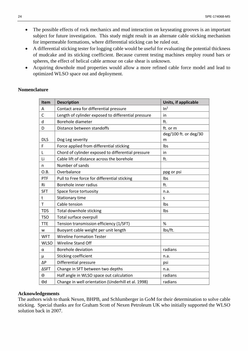
Nomenclature

Item Description Units, if applicable

A Contact area for differential pressure In2

C Length of cylinder exposed to differential pressure in

d Borehole diameter ft.

D Distance between standoffs ft. or m

DLS Dog Leg severity deg/100 ft. or deg/30 m

F Force applied from differential sticking lbs

L Chord of cylinder exposed to differential pressure in

Li Cable lift of distance across the borehole ft.

n Number of sands

O.B. Overbalance ppg or psi

PTF Pull to Free force for differential sticking lbs

Ri Borehole inner radius ft.

SFT Space force tortuosity n.a.

t Stationary time s

T Cable tension lbs

TDS Total downhole sticking lbs

TSO Total surface overpull

TTE Tension transmission efficiency (1/SFT) %

w Buoyant cable weight per unit length lbs/ft.

WFT Wireline Formation Tester

WLSO Wireline Stand Off

α Borehole deviation radians

µ Sticking coefficient n.a.

ΔP Differential pressure psi

ΔSFT Change in SFT between two depths n.a.

Ө Half angle in WLSO space out calculation radians

Өd Change in well orientation (Underhill et al. 1998) radians

Acknowledgements

The authors wish to thank Nexen, BHPB, and Schlumberger in GoM for their determination to solve cable

sticking. Special thanks are for Graham Scott of Nexen Petroleum UK who initially supported the WLSO

solution back in 2007.

SPE-174068-MS 25

References

Castillo, H., & Wills, P. (2007). SPE: 106562 Effective application of an innovative risk management methodology

to reduce well intervention cost and risks in long/deep/toruous wells. SPE.

Dupriest, F., Jr, W. E., & Ottesen, S. (2011). SPE: 128129 Design methodology and operational practices eliminate

differential sticking. SPE.

Evans, R., Brame, J., & Rose, L. C. (2007). SPE 108692: New innovative wireline jar adds significant value by

reducing fishing costs. SPE.

Johancsik, C., Frieson, D., & Dawson, R. (1983). JPT: Torque and drag in directional wells - prediction and

measurement. Journal of Petroleum technology.

Kemp, K., Elshahawi, H., Megat, A., Tollefsen, E., Kok, J., & S.Fey. (2011). SPWLA Analyzing the critical effects of

time on station. SPWLA 52nd Annual Logging Symposium.

McSpadden, A., Brown, P., & Davis, T. (2001). SPE 71560: Field Validation of 3-Dimensional Drag Model for

Tractor and Cable-Conveyed Well Intervention. SPE.

P. Isambourg, S. O. (1999). Down-Hole Simulation Cell for Measurement of Lubricity and Differential Pressure.

SPE/IADC 52816.

Prasad, T., Castillo, H., & Elshahawi, H. (2012). SPE: 159246 Effective mitigation fo tool sticking risk in formation

testing and fluid sampling operations. SPE.

Reid, P., Meeten, G., Way, P., Clark, P., Chambers, B., & Gilmour, A. (1996). SPE/IADC 35100 Mechanisms of

differential sticking and a simple well site test for monitoring and optimizing drilling mud properties. SPE.

Sarian, S., Varkey, J., Protasov, V., & Turner, J. (2013). SPE: 164762 Polymer-locked crush free wireline composite

cables reduce tool sticking and HSE risk in emerging deepwater reservoirs. SPE.

Underhill, W., Moore, L., & Meeten, G. (1998). SPE 48963: Model-Based Sticking Risk Assessment for Wireline

Formation Testing Tools in the Gulf coast. SPE.

Appendices

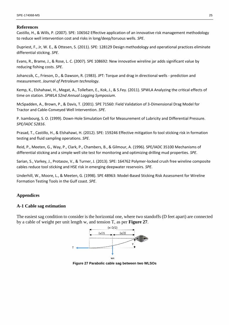
A-1 Cable sag estimation

The easiest sag condition to consider is the horizontal one, where two standoffs (D feet apart) are connected

by a cable of weight per unit length w, and tension T, as per Figure 27.

Figure 27 Parabolic cable sag between two WLSOs

26 SPE-174068-MS

Considering the moments about the end of the standoff:

𝑇𝑦 = (𝑤𝑥)𝑥

2,…………………………….(Eq.13)

𝑦 =𝑤𝑥2

2𝑇,…………………………….…..(Eq.14)

And when x = D/2 (the half distance between standoffs):

𝑦 =𝑤𝐷2

8𝑇,………………………(Eq.15)

For the deviated case, as illustrated below in Figure 28.

Figure 28 Parabolic cable sag between deviated WLSOs (normal sag [Sn] is towards formation and cake)

Since 𝒚 =𝒘𝒙𝟐

𝟐𝑻 then for two inclined standoffs located at (x1, y1) and (x2, y2):

𝒚𝟐 − 𝒚𝟏 = 𝑫𝒄𝒐𝒔𝜶 =𝒘(𝒙𝟐

𝟐−𝒙𝟏𝟐)

𝟐𝑻=

𝒘(𝒙𝟐−𝒙𝟏)(𝒙𝟐+𝒙𝟏)

𝟐𝑻,……………………(Eq.16)

∴ 𝑥2 + 𝑥1 = 𝐷𝑐𝑜𝑠𝛼2𝑇

𝑤 (𝑥2−𝑥1) ,………………………(Eq.17)

And 𝑥2 − 𝑥1 = 𝐷𝑠𝑖𝑛𝛼,…………………….(Eq.18)

From Eq.18 and Eq.19 x1 and x2 can be solved, by knowing D, T, w, and α.

The straight line between the standoffs can be defined by:

𝑦 = 𝑚𝑥 + 𝑐 ∴ 𝑐 = 𝑦 − 𝑚𝑥,……………(Eq.19)

And the constant c can be evaluated from either point (x1, y1) or (x2, y2):

Since 𝑚 =(𝒚𝟐−𝒚𝟏)

(𝒙𝟐−𝒙𝟏),…………………. (Eq.20)

SPE-174068-MS 27

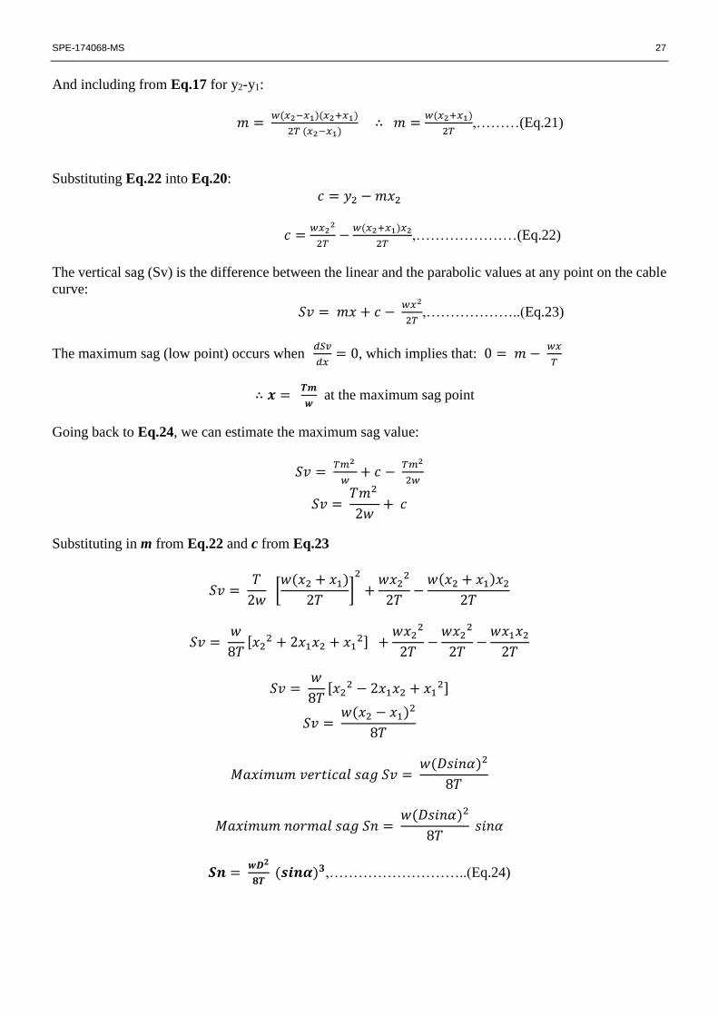
And including from Eq.17 for y2-y1:

𝑚 = 𝑤(𝑥2−𝑥1)(𝑥2+𝑥1)

2𝑇 (𝑥2−𝑥1) ∴ 𝑚 =

𝑤(𝑥2+𝑥1)

2𝑇,………(Eq.21)

Substituting Eq.22 into Eq.20:

𝑐 = 𝑦2 − 𝑚𝑥2

𝑐 =𝑤𝑥2

2

2𝑇−

𝑤(𝑥2+𝑥1)𝑥2

2𝑇,…………………(Eq.22)

The vertical sag (Sv) is the difference between the linear and the parabolic values at any point on the cable

curve:

𝑆𝑣 = 𝑚𝑥 + 𝑐 − 𝑤𝑥2

2𝑇,………………..(Eq.23)

The maximum sag (low point) occurs when 𝑑𝑆𝑣

𝑑𝑥= 0, which implies that: 0 = 𝑚 −

𝑤𝑥

𝑇

∴ 𝒙 = 𝑻𝒎

𝒘 at the maximum sag point

Going back to Eq.24, we can estimate the maximum sag value:

𝑆𝑣 = 𝑇𝑚2

𝑤+ 𝑐 −

𝑇𝑚2

2𝑤

𝑆𝑣 = 𝑇𝑚2

2𝑤+ 𝑐

Substituting in m from Eq.22 and c from Eq.23

𝑆𝑣 = 𝑇

2𝑤 [

𝑤(𝑥2 + 𝑥1)

2𝑇]

2

+𝑤𝑥2

2

2𝑇−

𝑤(𝑥2 + 𝑥1)𝑥2

2𝑇

𝑆𝑣 = 𝑤

8𝑇[𝑥2

2 + 2𝑥1𝑥2 + 𝑥12] +

𝑤𝑥22

2𝑇−

𝑤𝑥22

2𝑇−

𝑤𝑥1𝑥2

2𝑇

𝑆𝑣 = 𝑤

8𝑇[𝑥2

2 − 2𝑥1𝑥2 + 𝑥12]

𝑆𝑣 = 𝑤(𝑥2 − 𝑥1)2

8𝑇

𝑀𝑎𝑥𝑖𝑚𝑢𝑚 𝑣𝑒𝑟𝑡𝑖𝑐𝑎𝑙 𝑠𝑎𝑔 𝑆𝑣 = 𝑤(𝐷𝑠𝑖𝑛𝛼)2

8𝑇

𝑀𝑎𝑥𝑖𝑚𝑢𝑚 𝑛𝑜𝑟𝑚𝑎𝑙 𝑠𝑎𝑔 𝑆𝑛 = 𝑤(𝐷𝑠𝑖𝑛𝛼)2

8𝑇 𝑠𝑖𝑛𝛼

𝑺𝒏 = 𝒘𝑫𝟐

𝟖𝑻 (𝒔𝒊𝒏𝜶)𝟑,………………………..(Eq.24)

28 SPE-174068-MS

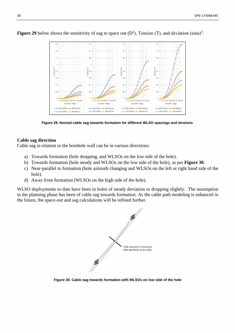
Figure 29 below shows the sensitivity of sag to space out (D2), Tension (T), and deviation (sinα)3.

Cable sag direction

Cable sag in relation to the borehole wall can be in various directions:

a) Towards formation (hole dropping, and WLSOs on the low side of the hole).

b) Towards formation (hole steady and WLSOs on the low side of the hole), as per Figure 30.

c) Near-parallel to formation (hole azimuth changing and WLSOs on the left or right hand side of the

hole).

d) Away from formation (WLSOs on the high side of the hole).

WLSO deployments to date have been in holes of steady deviation or dropping slightly. The assumption

in the planning phase has been of cable sag towards formation. As the cable path modeling is enhanced in

the future, the space-out and sag calculations will be refined further.

Figure 30. Cable sag towards formation with WLSOs on low side of the hole

Figure 29. Normal cable sag towards formation for different WLSO spacings and tensions