Social choice and voting theory - MIT OpenCourseWare
45
6.254: Game Theory with Engineering Applications Guest Lecture: Social Choice and Voting Theory Daron Acemoglu MIT May 6, 2010 1
Transcript of Social choice and voting theory - MIT OpenCourseWare
6.254: Game Theory with Engineering ApplicationsGuest Lecture: Social Choice and Voting Theory
Daron AcemogluMIT
May 6, 2010
1

Game Theory: Lecture 21 Introduction
Outline
Social choice and group decision-making
Arrow’s Impossibility Theorem
Gibbard-Satterthwaite Impossibility Theorem
Single peaked preferences and aggregation
Group decisions under incomplete information
Reading:
Microeconomic Theory, MasColell, Whinston and Green, Chapters 21 and 23.
2
1
2
3
Game Theory: Lecture 21 Group and Collective Choices
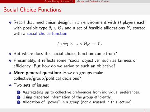
Social Choice Functions
Recall that mechanism design, in an environment with H players each with possible type θi ∈ Θ1 and a set of feasible alllocations Y , started with a social choice function
f : Θ1 × ... × ΘH → Y .
But where does this social choice function come from?
Presumably, it refiects some “social objective” such as fairness or effi ciency. But how do we arrive to such an objective?
More general question: How do groups makecollective/group/political decisions?
Two sets of issues:
Aggregating up to collective preferences from individual preferences. Using dispersed information of the group effi ciently. Allocation of “power” in a group (not discussed in this lecture).
3
Game Theory: Lecture 21 Group and Collective Choices
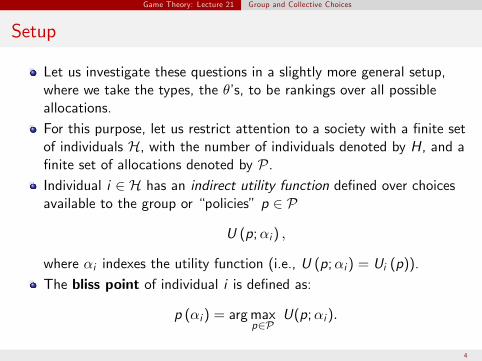
Setup
Let us investigate these questions in a slightly more general setup, where we take the types, the θ’s, to be rankings over all possible allocations. For this purpose, let us restrict attention to a society with a finite set of individuals H, with the number of individuals denoted by H, and a finite set of allocations denoted by P. Individual i ∈ H has an indirect utility function defined over choices available to the group or “policies” p ∈ P
U (p; αi ) ,
where αi indexes the utility function (i.e., U (p; αi ) = Ui (p)). The bliss point of individual i is defined as:
p (αi ) = argmax U(p; αi ). p∈P
4
Game Theory: Lecture 21 Group and Collective Choices
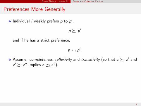
Preferences More Generally
Individual i weakly prefers p to p�,
p �i p�
and if he has a strict preference,
p �i p�.
Assume: completeness, refiexivity and transitivity (so that z �i z � and z � �i z �� implies z �i z ��).
5
Game Theory: Lecture 21 Group and Collective Choices
Collective Preferences?
Key question: Does there exist welfare function US (p) that ranks policies for this group (or society)?
Let us first start with a simple way of “aggregating” the preferences of individuals in the group: majoritarian voting.
This will lead to the Condorcet paradox.
6
Game Theory: Lecture 21 Voting and the Condorcet Paradox
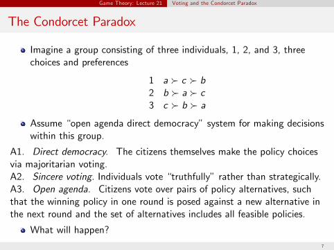
The Condorcet Paradox
Imagine a group consisting of three individuals, 1, 2, and 3, three choices and preferences
1 a � c � b 2 b � a � c 3 c � b � a
Assume “open agenda direct democracy” system for making decisions within this group.
A1. Direct democracy. The citizens themselves make the policy choices via majoritarian voting. A2. Sincere voting. Individuals vote “truthfully” rather than strategically. A3. Open agenda. Citizens vote over pairs of policy alternatives, such that the winning policy in one round is posed against a new alternative in the next round and the set of alternatives includes all feasible policies.
What will happen?
7
Game Theory: Lecture 21 Voting and the Condorcet Paradox
The Condorcet Paradox
It can be verified that b will obtain a majority against a.
c will obtain a majority against b.
But a will obtain a majority against c .
Thus there will be a cycle.
8
� �
Game Theory: Lecture 21 Arrow’s Theorem
Towards Collective Preferences
How general is the Condorcet cycle?
Arrow’s Impossibility Theorem: very general.
Suppose that the set of feasible policies is some finite set P.Let � be the set of all transitive orderings on P, that is, � containsinformation of the form p1 �i p2 �i p3 or p1 �i p2 �i p3, or orp1 �i p2 ∼i p3 and so on, and imposes the requirement of transitivityon these individual preferences.
An individual ordering Ri is an element of �, that is, Ri ∈ �.Since our society consists of H individuals, ρ = (R1, ..., RH ) ∈ �H is apreference profile.
Also ρ|P � = R1|P � , ..., RH |P � is the society’s preference profile when alternatives are restricted to some subset P � of P.
9
� �
Game Theory: Lecture 21 Arrow’s Theorem
Restrictions on Collective Preferences I
Let � be the set of all refiexive and complete binary relations on P(but notice not necessarily transitive).
A social ordering RS ∈ � is therefore a refiexive and complete binary relation over all the policy choices in P:
φ : �H → �.
We have already imposed “unrestricted domain,” since no restriction on preference profiles.
A social ordering is weakly Paretian if
p �i p� for all i ∈ H = ⇒ p �S p�.
10
� �
Game Theory: Lecture 21 Arrow’s Theorem
Restrictions on Collective Preferences II
Given ρ, a subset D of H is decisive between p, p� ∈ P, if
p �i p� for all i ∈ D and p �i � p� for some i � ∈ D = ⇒ p �S p�
If D� ⊂ H is decisive between p, p� ∈ P for all preference profiles ρ ∈ �H , then it is dictatorial between p, p� ∈ P. D ⊂ H is decisive if it is decisive between any p, p� ∈ P
D� ⊂ H is dictatorial if it is dictatorial between any p, p� ∈ P. If D� ⊂ H is dictatorial and a singleton, then its unique element is a dictator.
11
� �
Game Theory: Lecture 21 Arrow’s Theorem
Restrictions on Collective Preferences III
A social ordering satisfies independence from irrelevant alternatives, if for any ρ and ρ� ∈ �H and any p, p� ∈ P,
ρ = ρ� = φ (ρ) = φ ρ� .|{p,p�} |{p,p�} ⇒ |{p,p�} |{p,p�}
This axiom states that if two preference profiles have the same choice over two policy alternatives, the social orderings that derive from these two preference profiles must also have identical choices over these two policy alternatives, regardless of how these two preference profiles differ for “irrelevant” alternatives.
While this condition (axiom) at first appears plausible, it is in fact a reasonably strong one. In particular, it rules out any kind of interpersonal “cardinal” comparisons– that is, it excludes information on how strongly an individual prefers one outcome versus another.
12
Game Theory: Lecture 21 Arrow’s Theorem
Arrow’s Impossibility Theorem
Theorem
( Arrow’s (Im)Possibility Theorem) Suppose there are at least three alternatives. Then if a social ordering, φ, is transitive, weakly Paretian and satisfies independence from irrelevant alternatives, it must be dictatorial.
An immediate implication of this theorem is that any set of minimal decisive individuals D within the society H must either be a singleton, that is, D = {i}, so that we have a dictatorial social ordering, or we have to live with intransitivities.
Also implicitly, political power must matter. If we wish transitivity, political power must be allocated to one individual or a set of individuals with the same preferences.
How do we proceed? Restrict preferences or restrict institutions. →
13
Game Theory: Lecture 21 Arrow’s Theorem
Proof of Arrow’s Impossibility Theorem I
Suppose to obtain a contradiction that there exists a non-dictatorial and weakly Paretian social ordering, φ, satisfying independence from irrelevant alternatives. Contradiction in two steps.
Step 1: Let a set J ⊂ H be strongly decisive between p1, p2 ∈ P if for any preference profile ρ ∈ �H with p1 �i p2 for all i ∈ J and p2 �j p1 for all j ∈ H\J , p1 �S p2 (H itself is strongly decisive since φ is weakly Paretian).
We first prove that if J is strongly decisive between p1, p2 ∈ P, then J is dictatorial (and hence decisive for all p, p� ∈ P and for all preference profiles ρ ∈ �H ).
To prove this, consider the restriction of an arbitrary preference profile ρ ∈ �H to ρ|{p1,p2 ,p3 } and suppose that we also have p1 �i p3 for all i ∈ J .
14
Game Theory: Lecture 21 Arrow’s Theorem
Proof of Arrow’s Impossibility Theorem II
Next consider an alternative profile ρ� , such that |{p1 ,p2,p3 }p1 ��i p2 ��i p3 for all i ∈ J and p2 ��i p1 and p2 ��i p3 for all i ∈ H\J .
Since J is strongly decisive between p1 and p2, p1 ��S p2. Moreover, since φ is weakly Paretian, we also have p2 ��S p3, and thus p1 ��S p2 ��S p3. Notice that ρ� did not specify the preferences of individuals |{p1 ,p2,p3 }i ∈ H\J between p1 and p3, but we have established p1 ��S p3 for ρ� . |{p1 ,p2,p3 }We can then invoke independence from irrelevant alternatives and conclude that the same holds for ρ|{p1 ,p2,p3 }, i.e., p1 �
S p3.
But then, since the preference profiles and p3 are arbitrary, it must be the case that J is dictatorial between p1 and p3.
15
Game Theory: Lecture 21 Arrow’s Theorem
Proof of Arrow’s Impossibility Theorem III
Next repeat the same argument for ρ and ρ� , except |{p1 ,p2,p4 } |{p1 ,p2 ,p4 }that now p4 �i p2 and p4 ��i p1 ��i p2 for i ∈ J , while p2 ��j p1 and p4 ��j p1 for all j ∈ H\J .
Then, the same chain of reasoning, using the facts that J is strongly decisive, p1 ��S p2, φ is weakly Paretian and satisfies independence from irrelevant alternatives, implies that J is dictatorial between p4 and p2 (that is, p4 �S p2 for any preference profile ρ ∈ �H ).
Now once again using independence from irrelevant alternatives and also transitivity, for any preference profile ρ ∈ �H , p4 �i p3 for all i ∈ J .
Since p3, p4 ∈ P were arbitrary, this completes the proof that J is dictatorial (i.e., dictatorial for all p, p� ∈ P).
16
Game Theory: Lecture 21 Arrow’s Theorem
Proof of Arrow’s Impossibility Theorem IV
Step 2: Given the result in Step 1, if we prove that some individual h ∈ H is strongly decisive for some p1, p2 ∈ P, we will have established that it is a dictator and thus φ is dictatorial. Let Dab be the strongly decisive set between pa and pb .
Such a set always exists for any pa, pb ∈ P, since H is itself a strongly decisive set. Let D be the minimal strongly decisive set (meaning the strongly decisive set with the fewest members).
This is also well-defined, since there is only a finite number of individuals in H. Moreover, without loss of generality, suppose that D = D12 (i.e., let the strongly decisive set between p1 and p2 be the minimal strongly decisive set).
If D a singleton, then Step 1 applies and implies that φ is dictatorial, completing the proof.
17
Game Theory: Lecture 21 Arrow’s Theorem
Proof of Arrow’s Impossibility Theorem V
Thus suppose that D � Then, by unrestricted domain, the = {i}.following preference profile (restricted to {p1, p2, p3}) is feasible
for i ∈ D p1 �i p2 �i p3 for j ∈ D\{i} p3 �j p1 �j p2 for k / p2 �k p3 �k p1.∈ D
By hypothesis, D is strongly decisive between p1 and p2 and therefore Sp1 � p2.
Next if p3 �S p2, then given the preference profile here, D\{i} would be strongly decisive between p2 and p3, and this would contradict that D is the minimal strongly decisive set.
18
Game Theory: Lecture 21 Arrow’s Theorem
Proof of Arrow’s Impossibility Theorem VI
Thus p2 �S p3. Combined with p1 �S p2, this implies p1 �S p3. But given the preference profile here, this implies that {i} is strongly decisive, yielding another contradiction.
Therefore, the minimal strongly decisive set must be a singleton {h}for some h ∈ H. Then, from Step 1, {h} is a dictator and φ is dictatorial, completing the proof.
19
Game Theory: Lecture 21 Gibbard-Satterthwaite Theorem
Gibbard-Satterthwaite Theorem
Another issue: so far, we have assumed that people will express their preferences truthfully. But in the same way that we have to ensure truthfulness in implementing mechanisms, we have to make sure that our social choice rules provide incentives to report preferences truthfully.
We say that a social ordering φ : �H → � is strategy proof if when φ is being implemented, all individuals have a dominant strategy of representing their preferences truthfully.
More explicitly, we now have a game, in which each individual reports preference profile Rıi ∈ � but Rıi need not be the same as the true preference of this individual, Ri .
Question: What types of restrictions does strategy proofness impose?
20
Game Theory: Lecture 21 Gibbard-Satterthwaite Theorem
Gibbard-Satterthwaite Theorem
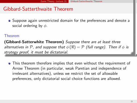
Suppose again unrestricted domain for the preferences and denote a social ordering by φ.
Theorem
(Gibbard-Satterwhite Theorem) Suppose there are at least three alternatives in P, and suppose that φ (�) = P (full range). Then if φ is strategy proof, it must be dictatorial.
This theorem therefore implies that even without the requirement of Arrow Theorem (in particular, weak Paretian and independence of irrelevant alternatives), unless we restrict the set of allowable preferences, only dictatorial social choice functions are allowed.
21
� �
Game Theory: Lecture 21 Gibbard-Satterthwaite Theorem
Proof of Gibbard-Satterthwaite Theorem
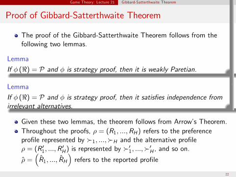
The proof of the Gibbard-Satterthwaite Theorem follows from the following two lemmas.
Lemma
If φ (�) = P and φ is strategy proof, then it is weakly Paretian.
Lemma
If φ (�) = P and φ is strategy proof, then it satisfies independence from irrelevant alternatives.
Given these two lemmas, the theorem follows from Arrow’s Theorem. Throughout the proofs, ρ = (R1, ..., RH ) refers to the preference profile represented by �1, ..., �H and the alternative profile ρ = (R1
� , ..., RH� ) is represented by ��1, ..., ��H , and so on.
ı Rı1, ..., ı refers to the reported profile ρ = RH
22
Game Theory: Lecture 21 Gibbard-Satterthwaite Theorem
Proof of First Lemma
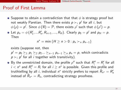
Suppose to obtain a contradiction that that φ is strategy proof but not weakly Paretian. Then there exists p �i p� for all i , but φ (ρ) = p�. Since φ (�) = P, there exists ρ� such that φ (ρ�) = p.
Let pn = φ (R1� , ...Rn
� , Rn+1, ..., RH ). Clearly p0 = p� and pH = p. Then
n∗ = min {H ≥ n > 0 : pn �n pn−1}
exists (suppose not, then p� = p0 �1 p1 �2 p2... �n−1 pn−1 �n pn = p, which contradicts p �i p� for all i together with transitivity).
By the unrestricted domain, the profile ρ�� such that Ri�� = Ri
� for all i < n∗ and Ri
�� = Ri for all i ≥ n∗ is possible. Given this profile and truthtelling by all i , individual n∗ strictly prefers to report Rın∗ = Rn
�
instead of Rın∗ = Rn , contradicting strategy proofness.
23
Game Theory: Lecture 21 Gibbard-Satterthwaite Theorem
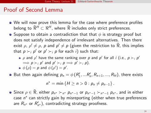
Proof of Second Lemma
We will now prove this lemma for the case where preference profiles belong to �̄H ⊂ �H , where � ¯ includes only strict preferences. Suppose to obtain a contradiction that that φ is strategy proof but does not satisfy independence of irrelevant alternatives. Then there exist ρ, ρ� =� ρ, p and p� =� p (given the restriction to �̄, this implies that p �i p� or p� �i p for each i) such that:
ρ and ρ� have the same ranking over p and p� for all i (i.e., p �i p� = ⇒ p �i p� and p� �i p = ⇒ p� �i p). φ (ρ) = p and φ (ρ�) = p�.
But then again defining pn = φ (R1� , ...Rn
� , Rn+1, ..., RH ), there exists
n∗ = min {H ≥ n > 0 : pn =� pn−1} .
Since ρ ∈ �̄, either pn∗ �n∗ pn∗−1 or pn∗−1 �n∗−1 pn∗ , and in either case n∗ can strictly gain by misreporting (either when true preferences are Rn∗ or Rn
�∗ ), contradicting strategy proofness.
24
Game Theory: Lecture 21 Gibbard-Satterthwaite Theorem
Proof of Gibbard-Satterthwaite Theorem
The two lemmas together imply that when preference profiles belong to �̄H , strategy proofness implies a dictatorial social choice function, say with the dictator given by individual i∗.
The proof of theorem is completed by showing that on the domain �H , if i∗ is not a dictator, then either i∗ or another individual would have a strict incentive to misreport.
25
Game Theory: Lecture 21 Single-Peaked Preferences and the Median Voter Theorem
The Condorcet Winner
We can avoid the Condorcet paradox when there is a Condorcet winner.
Definition
A Condorcet winner is a policy p∗ that beats any other feasible policy in a pairwise vote.
26
Game Theory: Lecture 21 Single-Peaked Preferences and the Median Voter Theorem
Single-Peaked Preferences
Suppose P ⊂ R.
Definition
Consider a finite set of P ⊂ R and let p(αi ) ∈ P be individual i’s unique bliss point over P. Then, the policy preferences of citizen i are single peaked iff:
For all p��, p� ∈ P, such that p�� < p� ≤ p(αi ) or p�� > p� ≥ p(αi ),
we have U(p��; αi ) < U(p�; αi ).
Essentially strict quasi-concavity of U Median voter: rank all individuals according to their bliss points, the p (αi )’s. Suppose that H odd. Then, the median voter is the individual who has exactly (H − 1) /2 bliss points to his left and (H − 1) /2 bliss points to his right. Denote this individual by αm , and his bliss point (ideal policy) by pm .
27
Game Theory: Lecture 21 Single-Peaked Preferences and the Median Voter Theorem
Median Voter Theorem
Theorem
(The Median Voter Theorem) Suppose that H is an odd number, that A1 and A2 hold and that all voters have single-peaked policy preferences over a given ordering of policy alternatives, P. Then, a Condorcet winner always exists and coincides with the median-ranked bliss point, pm. Moreover, pm is the unique equilibrium policy (stable point) under the open agenda majoritarian rule, that is, under A1-A3.
This also immediately implies:
Corollary
With single peaked preferences, there exists a social ordering φ that satisfies independence from irrelevant alternatives and that is transitive, weakly Paretian and non-dictatorial.
28
Game Theory: Lecture 21 Single-Peaked Preferences and the Median Voter Theorem
Proof of the Median Voter Theorem
The proof is by a “separation argument”.
Order the individuals according to their bliss points p(αi ), and label the median-ranked bliss point by pm .
By the assumption that H is an odd number, pm is uniquely defined (though αm may not be uniquely defined).
Suppose that there is a vote between pm and some other policy p�� < pm .
By definition of single-peaked preferences, for every individual with pm < p(αi ), we have U (pm ; αi ) > U (p��; αi ).
By A2, these individuals will vote sincerely and thus, in favor of pm .
The coalition voting for supporting pm thus constitutes a majority.
The argument for the case where p�� > pm is identical.
29
Game Theory: Lecture 21 Single-Peaked Preferences and the Median Voter Theorem
Median Voter Theorem: Discussion
Odd number of individuals to shorten the statement of the theorem and the proof.
It is straightforward to generalize the theorem and its proof to the case in which H is an even number.
More important: does it also help us against theGibbard-Satterthwaite Theorem?
The answer is Yes.
In particular, with single peaked preferences, sincere voting (truthful revelation of preferences) is optimal, which implies strategy proofness.
30
Game Theory: Lecture 21 Single-Peaked Preferences and the Median Voter Theorem
Strategic Voting
A2�. Strategic voting. Define a vote function of individual i in a pairwise contest between p� and p�� by vi (p�, p��) ∈ {p�, p��}. Let a voting (counting) rule in a society with H citizens be V :{p�, p��} H → {p�, p��} for any p�, p�� ∈ P. Let V (vi (p�, p��) , v−i (p�, p��)) be the policy outcome from voting rule V applied to the pairwise contest {p�, p��}, when the remaining individuals cast their votes according to the vector v−i (p�, p��), and when individual i votes vi (p�, p��). Strategic voting means that � � � � � � � �� �
vi p�, p�� ∈ arg max U V v̂i p�, p�� , v−i p�, p�� ; αi . v̂i (p�,p��)
Recall that a weakly-dominant strategy for individual i is a strategy that gives weakly higher payoff to individual i than any of his other strategies regardless of the strategy profile of other players.
31
Game Theory: Lecture 21 Single-Peaked Preferences and the Median Voter Theorem
Median Voter Theorem with Strategic Voting
Theorem
(The Median Voter Theorem With Strategic Voting) Suppose that H is an odd number, that A1 and A2� hold and that all voters have single-peaked policy preferences over a given ordering of policy alternatives, P. Then, sincere voting is a weakly-dominant strategy for each player and there exists a unique weakly-dominant equilibrium, which features the median-ranked bliss point, pm, as the Condorcet winner.
Notice no more “open agenda”. Why not?
Why emphasis on weakly-dominant strategies?
32
Game Theory: Lecture 21 Single-Peaked Preferences and the Median Voter Theorem
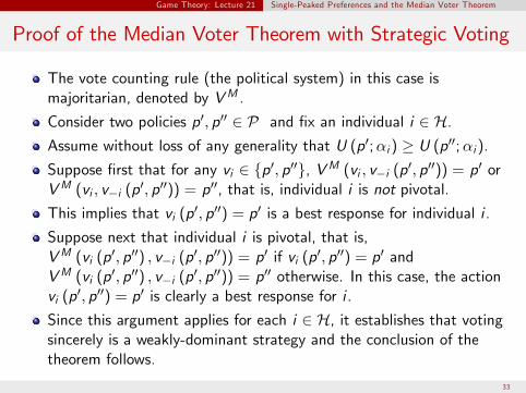
Proof of the Median Voter Theorem with Strategic Voting
The vote counting rule (the political system) in this case ismajoritarian, denoted by VM .
Consider two policies p�, p�� ∈ P and fix an individual i ∈ H.Assume without loss of any generality that U (p�; αi ) ≥ U (p��; αi ).
Suppose first that for any vi ∈ {p�, p��}, VM (vi , v−i (p�, p��)) = p� orVM (vi , v−i (p�, p��)) = p��, that is, individual i is not pivotal.
This implies that vi (p�, p��) = p� is a best response for individual i .
Suppose next that individual i is pivotal, that is,VM (vi (p�, p��) , v−i (p�, p��)) = p� if vi (p�, p��) = p� andVM (vi (p�, p��) , v−i (p�, p��)) = p�� otherwise. In this case, the actionvi (p�, p��) = p� is clearly a best response for i .
Since this argument applies for each i ∈ H, it establishes that votingsincerely is a weakly-dominant strategy and the conclusion of thetheorem follows.
33
Game Theory: Lecture 21 Single-Peaked Preferences and the Median Voter Theorem
Strategic Voting in Sequential Elections
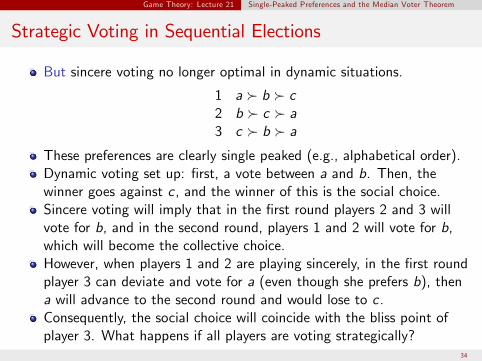
But sincere voting no longer optimal in dynamic situations.
1 a � b � c2 b � c � a 3 c � b � a
These preferences are clearly single peaked (e.g., alphabetical order). Dynamic voting set up: first, a vote between a and b. Then, the winner goes against c , and the winner of this is the social choice. Sincere voting will imply that in the first round players 2 and 3 will vote for b, and in the second round, players 1 and 2 will vote for b, which will become the collective choice. However, when players 1 and 2 are playing sincerely, in the first round player 3 can deviate and vote for a (even though she prefers b), then a will advance to the second round and would lose to c . Consequently, the social choice will coincide with the bliss point of player 3. What happens if all players are voting strategically?
34
Game Theory: Lecture 21 Single-Peaked Preferences and the Median Voter Theorem
Strategy Proofness with Single Peaked Preferences
The above example notwithstanding, single peaked preferences are suffi cient to ensure strategy proofness. In particular:
Theorem
Suppose preferences are single peaked. Then there exists a social choice rule φ that is strategy proof.
Moreover, it can be shown that in this case strategy proofness implies that the social choice rule must be an “augmented median voter” rule, which essentially selects the median from a list of the bliss points of all individuals augmented by additional choices (so a dictatorial social choice rule as well as certain other rules are augmented median voter rules).
35
Game Theory: Lecture 21 Juries
Group Decisions under Incomplete Information
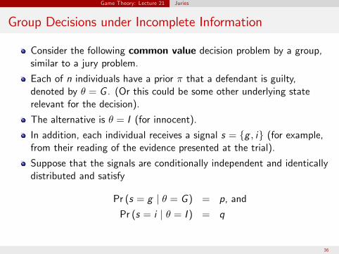
Consider the following common value decision problem by a group, similar to a jury problem.
Each of n individuals have a prior π that a defendant is guilty, denoted by θ = G . (Or this could be some other underlying state relevant for the decision).
The alternative is θ = I (for innocent).
In addition, each individual receives a signal s = {g , i} (for example, from their reading of the evidence presented at the trial).
Suppose that the signals are conditionally independent and identically distributed and satisfy
Pr (s = g | θ = G ) = p, and
Pr (s = i | θ = I ) = q
36
Game Theory: Lecture 21 Juries
Decisions and Payoffs
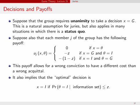
Suppose that the group requires unanimity to take a decision x = G . This is a natural assumption for juries, but also applies in many situations in which there is a status quo. Suppose also that each member j of the group has the following payoff: ⎧ ⎨ 0 if x = θ
uj (x , θ) = ⎩ −z if x = G and θ = I
− (1 − z) if x = I and θ = G
This payoff allows for a wrong conviction to have a different cost than a wrong acquittal.
It also implies that the “optimal” decision is
x = I if Pr (θ = I | information set) ≤ z .
37
�
��
��
Game Theory: Lecture 21 Juries
Bayesian Nash Equilibrium
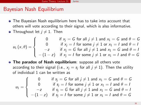
The Bayesian Nash equilibrium here has to take into account that others will vote according to their signal, which is also informative. Throughout let j = 1. Then ⎧ ⎪⎪⎨ ⎪⎪⎩
0 if xj = G for all j =� 1 and x1 = G and θ = G 0 if xj = I for some j =� 1 or x1 = I and θ = I
= 1 and x1 = I for some j
u1 (x , θ) = if xj = G for all j = G and θ = I−z
− (1 − z) if xj = 1 or x1 = I and θ = G
The paradox of Nash equilibrium: suppose all others vote according to their signal (i.e., xj = sj for all j =� 1). Then the utility of individual 1 can be written as ⎧ ⎪⎪⎨ ⎪⎪⎩
0 if sj = G for all j =� 1 and x1 = G and θ = G 0 if sj = I for some j =� 1 or x1 = I and θ = I
= 1 and x1 u1 =
if sj = G for all j = G and θ = I= 1 or x1 = I and θ = G
−z− (1 − z) = I for some jif sj
38
Game Theory: Lecture 21 Juries
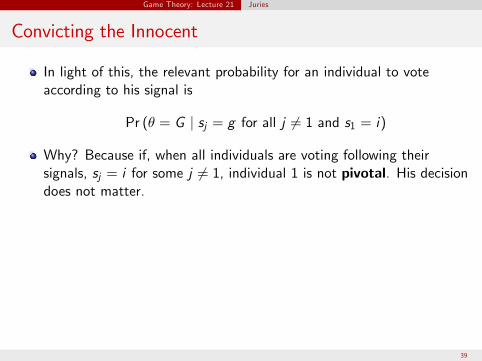
Convicting the Innocent
In light of this, the relevant probability for an individual to vote according to his signal is
Pr (θ = G | sj = g for all j =� 1 and s1 = i)
Why? Because if, when all individuals are voting following their signals, sj = i for some j =� 1, individual 1 is not pivotal. His decision does not matter.
39
= �
Game Theory: Lecture 21 Juries
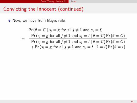
Convicting the Innocent (continued)
Now, we have from Bayes rule
Pr (θ = G | sj = g for all j =� 1 and s1 = i) Pr (sj = g for all j = 1 and s1 = i | θ = G ) Pr (θ = G )
Pr (sj = g for all j =� 1 and s1 = i | θ = G ) Pr (θ = G ) + Pr (sj = g for all j =� 1 and s1 = i | θ = I ) Pr (θ = I )
40
Game Theory: Lecture 21 Juries
Convicting the Innocent (continued)
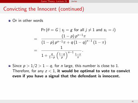
Or in other words
Pr (θ = G | sj = g for all j =� 1 and s1 = i)
(1 − p) pn−1π =
(1 − p) pn−1π + q (1 − q)n−1 (1 − π) 1
= 1 + q
� 1−q
�n−11−π
.
1−p p π
Since p > 1/2 > 1 − q, for n large, this number is close to 1. Therefore, for any z < 1, it would be optimal to vote to convict even if you have a signal that the defendant is innocent.
41
Game Theory: Lecture 21 Juries
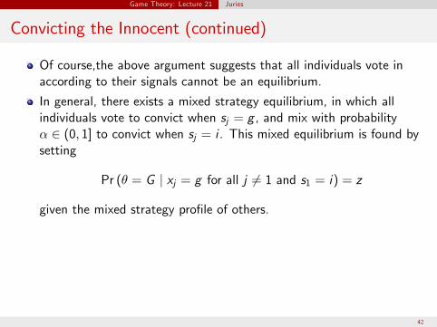
Convicting the Innocent (continued)
Of course,the above argument suggests that all individuals vote in according to their signals cannot be an equilibrium.
In general, there exists a mixed strategy equilibrium, in which all individuals vote to convict when sj = g , and mix with probability α ∈ (0, 1] to convict when sj = i . This mixed equilibrium is found by setting
Pr (θ = G | xj = g for all j =� 1 and s1 = i) = z
given the mixed strategy profile of others.
42
= � �
Game Theory: Lecture 21 Juries
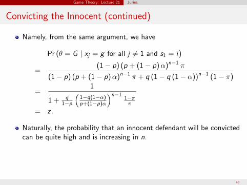
Convicting the Innocent (continued)
Namely, from the same argument, we have
Pr (θ = G | xj = g for all j =� 1 and s1 = i)
(1 − p) (p + (1 − p) α)n−1 π =
(1 − p) (p + (1 − p) α)n−1 π + q (1 − q (1 − α))n−1 (1 − π) 1
q 1−q(1−α) n−1 1−π1 + 1−p p+(1−p)α π
= z .
Naturally, the probability that an innocent defendant will be convicted can be quite high and is increasing in n.
43
Game Theory: Lecture 21 Juries
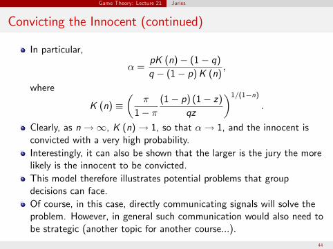
Convicting the Innocent (continued)
In particular, pK (n) − (1 − q)
α = , q − (1 − p) K (n)
where � π (1 − p) (1 − z)
�1/(1−n)K (n) ≡
1 − π qz .
Clearly, as n →∞, K (n) → 1, so that α → 1, and the innocent is convicted with a very high probability. Interestingly, it can also be shown that the larger is the jury the more likely is the innocent to be convicted. This model therefore illustrates potential problems that group decisions can face. Of course, in this case, directly communicating signals will solve the problem. However, in general such communication would also need to be strategic (another topic for another course...).
44

MIT OpenCourseWarehttp://ocw.mit.edu
6.254 Game Theory with Engineering Applications Spring 2010
For information about citing these materials or our Terms of Use, visit: http://ocw.mit.edu/terms.