Small Signal Stability Analysis of Power System Network...
13
Australian Journal of Basic and Applied Sciences, 7(11) Sep 2013, Pages: 375-387 AENSI Journals Australian Journal of Basic and Applied Sciences Journal home page: www.ajbasweb.com Corresponding Author: Agileswari K. Ramasamy, College of Engineering, Universiti Tenaga Nasional E-mail: [email protected] Small Signal Stability Analysis of Power System Network with Varying Load, Line and Generation Parameters Agileswari Ramasamy, Hemalan Nambier Vijayan College of Engineering, Universiti Tenaga Nasional ARTICLE INFO ABSTRACT Article history: Received 4 September 2013 Received in revised form 21 October 2013 Accepted 29October 2013 Available online 18 November 2013 Key words: Eigen-analysis, participation factor, small signal stability. Stability issues are of concern in modern day power systems. Small signal stability issues cause small perturbations in the generator that can result in instability of the power network. Generally, small signal stability issues are related to the generator and load properties of a power system. This paper examines the effects of load variations and line length variations on a power system network, in terms of its oscillation for a small signal stability study. Eigenvalues and eigenvectors are used to examine and analysis the stability of the power system. The dynamic power system's mathematical model is constructed and thus calculated using load flow and small signal stability toolbox on MATLAB. The power system model is based on a 3-machine 9-bus system that was modified to suit this study. In this paper, Participation Factors are a means to gauge the effects of variation in these conditions with respect to the stability parameters on the network. © 2013 AENSI Publisher All rights reserved. INTRODUCTION In power systems networks, reliability and security are among the main concerns for a continuously growing global power market. With implementation of power electronic equipment such as power system stabilizers and metering devices to monitor and mitigate this concerns, power system networks are able to expand and sometimes even link with other large networks, which are called as interconnecting networks. Interconnection of power system networks are a well-established practice generally for technical and economic reasons. Generators usually experience oscillatory problems throughout its usage and can be risky to the system in terms of disturbing continuous power transfer to the grid. One such oscillatory problem is the small signal stability issue, which is caused by small perturbations in the system, which, occurs frequently in normal systems (El Amin et al.,1994, Kundur P et al.,2004,L.T.G Lima et al.,1995). A method of small signal stability analysis uses the modal analysis method where investigation is done on the modes (eigenvalues) and states (electrical and mechanical parameters of a generator). Modes of a system can either be underdamped (unstable) or marginally stable. Particularly, analysis is done on the least damped mode (as in a case of instability of the system) to determine its type of oscillation, source of oscillation and its response to changes in system parameter values (J. Ma et al.,2006, G. Angelidis et al.,1996, Y.V. Makarov et al.,1998,L.H Bezerra and C.Tomei,1999). This paper investigates different parameters of a power system network for small signal stability effects. Firstly, the modeling of the system is presented then the various simulations on a test network are included. Finally, the results achieved are discussed. The results will show which power system network parameters have an explicit effect on small signal stability. Modeling Dynamic Oscillation: With electrical power systems, the change of electrical torque of a machine after a perturbation can be determined in two parts:- D s e T T T (1.1) T S ∆δ is the component of torque change in phase with rotor angle perturbation, ∆δ and is referred to as the synchronizing torque component. T S is the synchronous torque coefficient. T D ∆ω is the component of torque in phase with speed deviation, ∆ω and is referred to as damping torque component. T D is the damping torque coefficient (Kundur P et al.,2004, Richard G Farmer, 2006, Kundur P et al., 1989).
Transcript of Small Signal Stability Analysis of Power System Network...

Australian Journal of Basic and Applied Sciences, 7(11) Sep 2013, Pages: 375-387
AENSI Journals
Australian Journal of Basic and Applied Sciences
Journal home page: www.ajbasweb.com
Corresponding Author: Agileswari K. Ramasamy, College of Engineering, Universiti Tenaga Nasional
E-mail: [email protected]
Small Signal Stability Analysis of Power System Network with Varying Load, Line and
Generation Parameters
Agileswari Ramasamy, Hemalan Nambier Vijayan
College of Engineering, Universiti Tenaga Nasional
A R T I C L E I N F O A B S T R A C T
Article history:
Received 4 September 2013 Received in revised form 21 October 2013 Accepted 29October 2013 Available online 18 November 2013
Key words:
Eigen-analysis, participation factor,
small signal stability.
Stability issues are of concern in modern day power systems. Small signal stability
issues cause small perturbations in the generator that can result in instability of the
power network. Generally, small signal stability issues are related to the generator and
load properties of a power system. This paper examines the effects of load variations
and line length variations on a power system network, in terms of its oscillation for a
small signal stability study. Eigenvalues and eigenvectors are used to examine and
analysis the stability of the power system. The dynamic power system's mathematical
model is constructed and thus calculated using load flow and small signal stability
toolbox on MATLAB. The power system model is based on a 3-machine 9-bus system
that was modified to suit this study. In this paper, Participation Factors are a means to
gauge the effects of variation in these conditions with respect to the stability parameters
on the network.
© 2013 AENSI Publisher All rights reserved.
INTRODUCTION
In power systems networks, reliability and security are among the main concerns for a continuously
growing global power market. With implementation of power electronic equipment such as power system
stabilizers and metering devices to monitor and mitigate this concerns, power system networks are able to
expand and sometimes even link with other large networks, which are called as interconnecting networks.
Interconnection of power system networks are a well-established practice generally for technical and economic
reasons. Generators usually experience oscillatory problems throughout its usage and can be risky to the system
in terms of disturbing continuous power transfer to the grid. One such oscillatory problem is the small signal
stability issue, which is caused by small perturbations in the system, which, occurs frequently in normal systems
(El Amin et al.,1994, Kundur P et al.,2004,L.T.G Lima et al.,1995).
A method of small signal stability analysis uses the modal analysis method where investigation is done on
the modes (eigenvalues) and states (electrical and mechanical parameters of a generator). Modes of a system can
either be underdamped (unstable) or marginally stable. Particularly, analysis is done on the least damped mode
(as in a case of instability of the system) to determine its type of oscillation, source of oscillation and its
response to changes in system parameter values (J. Ma et al.,2006, G. Angelidis et al.,1996, Y.V. Makarov et
al.,1998,L.H Bezerra and C.Tomei,1999).
This paper investigates different parameters of a power system network for small signal stability effects.
Firstly, the modeling of the system is presented then the various simulations on a test network are included.
Finally, the results achieved are discussed. The results will show which power system network parameters have
an explicit effect on small signal stability.
Modeling Dynamic Oscillation:
With electrical power systems, the change of electrical torque of a machine after a perturbation can be
determined in two parts:-
Dse TTT
(1.1)
TS∆δ is the component of torque change in phase with rotor angle perturbation, ∆δ and is referred to as the
synchronizing torque component. TS is the synchronous torque coefficient. TD∆ω is the component of torque in
phase with speed deviation, ∆ω and is referred to as damping torque component. TD is the damping torque
coefficient (Kundur P et al.,2004, Richard G Farmer, 2006, Kundur P et al., 1989).
376 Agileswari K. Ramasamy and Hemalan Nambier Vijayan et al, 2013
Australian Journal of Basic and Applied Sciences, 7(11) Sep 2013, Pages: 375-387
For a system to maintain stability both of the above components are required. A lack of sufficient
synchronizing torque, TS will result in instability in the rotor angle,∆δ. The lack of sufficient damping torque, TD
results in oscillatory instability which affects the speed deviation of the machine,∆ω.
Modeling Dynamic Oscillation:
For a linear system, the general equation is given in (El Amin et al., 1994, Kundur P et al., 2004, L.T.G
Lima et al.,1995, L.H Bezerra and C.Tomei,1999, Richard G Farmer, 2006, Kundur P et al., 1989)
BuAxdt
dx
(1.2)
where
x is a vector of system states
A is a square matrix of dimension equal to the number of states
B is a matrix which defines the proportion of each input that is applied to each state equation
u is a vector of system inputs
The system’s output is generally expressed as
DuCxy (1.3)
y is a vector of system outputs
C is the output matrix
D is the feed forward matrix
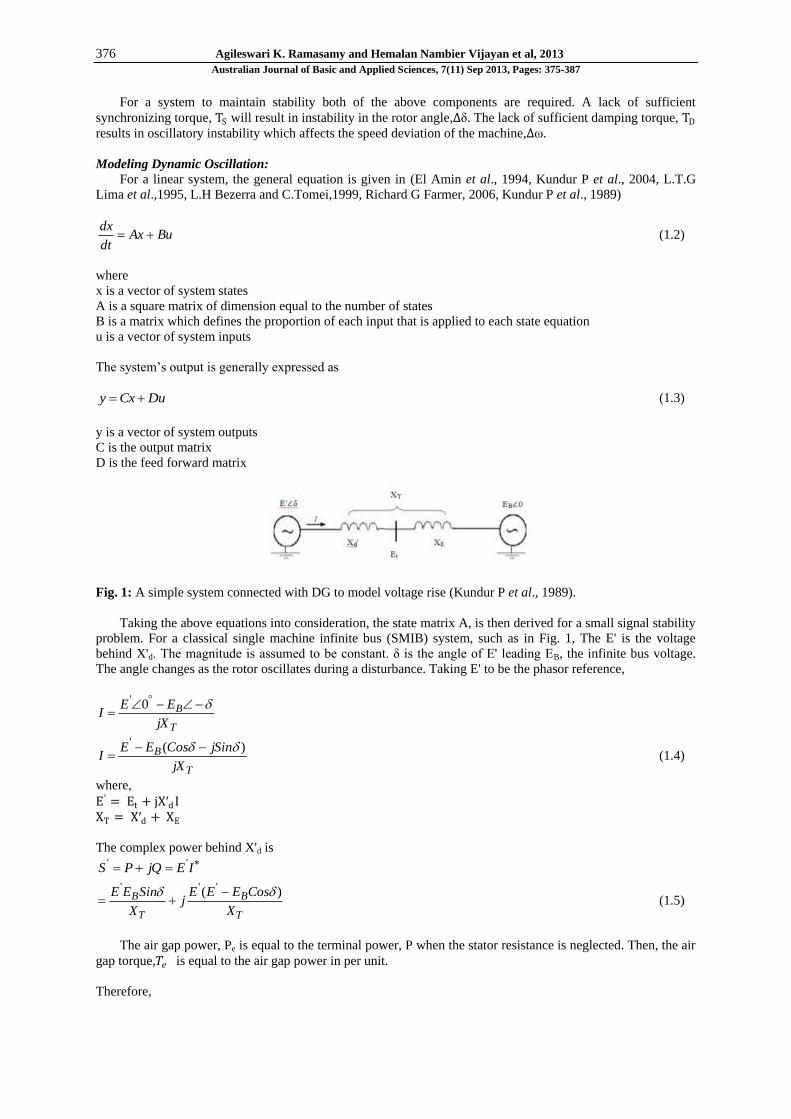
Fig. 1: A simple system connected with DG to model voltage rise (Kundur P et al., 1989).
Taking the above equations into consideration, the state matrix A, is then derived for a small signal stability
problem. For a classical single machine infinite bus (SMIB) system, such as in Fig. 1, The E' is the voltage
behind X'd. The magnitude is assumed to be constant. δ is the angle of E' leading EB, the infinite bus voltage.
The angle changes as the rotor oscillates during a disturbance. Taking E' to be the phasor reference,
T
B
jX
EEI
0'
T
B
jX
jSinCosEEI
)(' (1.4)
where,
E′ = Et + jX′d I XT = X′d + XE
The complex power behind X'd is IEjQPS ''
T
B
T
B
X
CosEEEj
X
SinEE )( '''
(1.5)
The air gap power, Pe is equal to the terminal power, P when the stator resistance is neglected. Then, the air
gap torque,𝑇𝑒 is equal to the air gap power in per unit.
Therefore,
377 Agileswari K. Ramasamy and Hemalan Nambier Vijayan et al, 2013
Australian Journal of Basic and Applied Sciences, 7(11) Sep 2013, Pages: 375-387
T
Bee
X
SinEEPPT
'
(1.6)
Assume initial operating condition, δ = δo, linearizing it unfolds,
e
eT
T
T
B
X
CosEE '
(1.7)
Keeping these equations aside, consider the standard equations of motion for power system stability,
derived to include inertia constant and damping torque component is
rDem KTTdt
dH
2
22 (1.8)
This swing equation is further expressed as two first order differential equations,
)(2
1rDem
r KTTHdt
d
(1.9)
rdt
d
From the above equations, time t is in seconds, the rotor angle, δ (angle by which 𝐸′leads𝐸𝐵) is in electrical
radians and 𝜔0 is equal to 2πf. 𝑇𝑒 is the electrical torque and 𝑇𝑚 is the mechanical torque. These variable
including ∆𝜔𝑟 is assumed to be in per unit. Now linearizing equation 1.9 and replacing for Δ𝑇𝑒 given in
equation 1.7,
)(2
1rDsm
r KKTHdt
d
(1.10)
where Ks is the synchronizing torque coefficient given as
T
BS
X
CosEEK
'
(1.11)
Now linearizing equation 1.10:-,
rdt
d
(1.12)
Equations 1.10 and 1.12 are written in the vector-matrix form, obtains
mr
SDr THH
K
H
K
dt
d
02
1
022
(1.13)
Therefore equation 1.13 is of the form 𝐱 = 𝐀𝐱 + 𝐁𝑢 where the state matrix A elements are dependent on
KD, KT, H which are the system parameters and E' and δ0 which are the initial operating conditions.
Eigen-analysis:
The Small Signal Stability analysis of an electrical power system is examined by the eigenvalues of the
state matrix A. These eigenvalues may be either real or complex values. A real eigenvalue will represent a non-
oscillatory mode, while a complex pair of eigenvalues corresponds to an oscillatory mode (K. Meerbergen et

378 Agileswari K. Ramasamy and Hemalan Nambier Vijayan et al, 2013
Australian Journal of Basic and Applied Sciences, 7(11) Sep 2013, Pages: 375-387
al.,1994, K.A Cliffe et al.,1994). The real part of complex eigenvalues provides the damping coefficient, while
the imaginary part gives the oscillation frequency. The eigenvalues, λ of the state matrix are given by the non-
trivial solutions of the equation 2.1.
0det I (2.1)
The ith right eigenvector satisfies
iii uu (2.2)
The ith left eigenvector satisfies
iii VV (2.3)
The most general representation of state-space for linear systems are given in equations 2.4 and 2.5
)()()()()( tutBtxtAtx (2.4)
)()()()()( tutDtxtCty (2.5)
Participation factors:
Participation factors are non-dimensional and easy to compute. The trouble with using left and right
eigenvectors independently is that they are dependent on units and scaling associated with the state variables.
They are a fast way to determine possible candidate machines for damping control of unstable or lightly stable
rotor angle oscillatory modes. Participation factors are a measure of the relative participation of the jth
eigenvalue (state variable) in the ith mode, and vice versa. The right eigenvector measures the activity of x in the
ith mode and left eigenvector weighs the contribution of this activity to the mode. The product of these Pji,
measures the net participation, as per equation 2.6. Participation factor is actually equal to the sensitivity of the
eigenvalue λj to the diagonal element of Ars of the state matrix A as in equation 2.7 (Hsu, Yuan-Yih et al.,
1987,Rodriguez, O. et al., 2007,Castrillon et al., 2012 )
)()( iuivP jjji (2.6)
)()( survA
jjrs
j
(2.7)
Simulation:
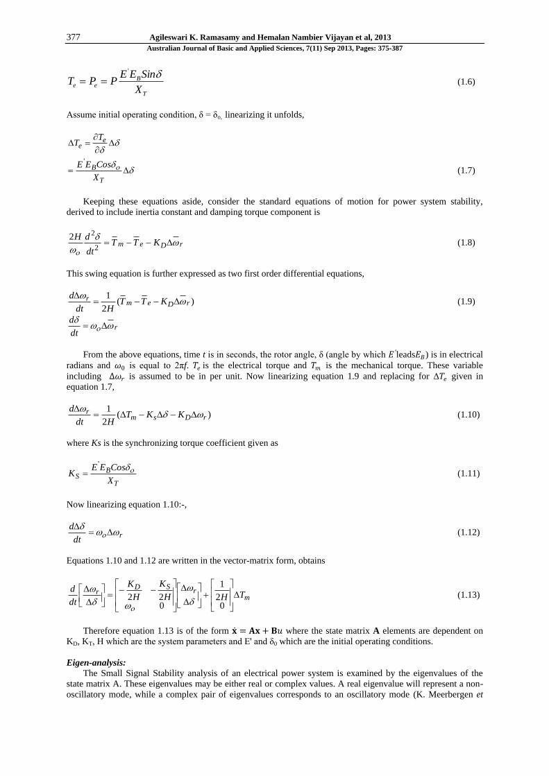
The test system used in this investigation is the IEEE – 3 machine 9 bus test system as in Fig.2 with
modifications so that the parameters of both left and right sides of the network mirror each other. The reason
this test network was modified such, was so that the effect of variations on its generation could be significantly
detected. The symmetrical distance of lines, and loads would help in indicating changes in dominant states as
well as stability as the generation varies. For example, the parameters for line distance of bus 2-7 is equal to bus
3-9, while bus 7-5 is similar to bus 9-6, and so on. MATLAB toolbox was used to analyze this system by
performing the small signal analysis. Small signal stability analysis is carried out by performing the following
steps:-
a) Loads the system data
b) Performs load flow on the system, linearizes system equations and construct the matrices and finally the
system state matrix A.
c) Calculate system’s eigenvalues, associated frequency and damping ratios.
The effect of load and line variation was analyzed by increasing the values of one parameter methodically
from 0%-150% of the original value. At each change in the values the state variables were re-calculated after
running a load flow program and linearization of the system equation was performed and the state matrix A.
Analysis of the system can then be carried out by acquiring the eigenvalues of the state matrix, A and the
associated participation factors. The eigenvectors are then used check for stability of swinging characteristics of
the system.
379 Agileswari K. Ramasamy and Hemalan Nambier Vijayan et al, 2013
Australian Journal of Basic and Applied Sciences, 7(11) Sep 2013, Pages: 375-387
Fig. 2: The 3 machine 9 bus test case.
RESULTS AND DISCUSSION
Table 1 shows the modes for the test system, its associated eigenvectors, the damping factor, frequency and
the dominant state for that particular mode based on participation factors. Of the dominant states, only the
electrical parameters are considered as they contribute to the rotational angle, δ and rotational speed, ω of the
generators (Blasco-Gimenez et al., 1996).
For the eigenvalues listed in Table 1, the complex values reflect an oscillatory mode while real eigenvalues
show a non-oscillatory mode. Therefore there are actually only 7 states for each of the generators. Only modes
12/13 and are considered for analysis as they have both complex eigenvalues, are related to an electrical
parameter of the generators and most importantly have the lowest damping ratio. The dominant state of each
mode is obtained using the participation factor. It shows the most influential state for that particular mode.
Although modes 1 and 2 are influenced by δ of generator 1 (an electrical parameter), still it is non-oscillatory,
and will not be taken into consideration for this type of stability problem (Kundur P et al.,2004).
Table 1: General Parameters For Test System.
Mode Eigenvectors Damping Factor Frequency, Hz Dominant States
1 -0.0024 1.0000 0 δ of Gen 1
2 0.0024 -1.0000 0
3 -0.5126 - 0.8143i 0.5328 0.1296 Mechanical parameters Gen 2
4 -0.5126 + 0.8143i 0.5328 0.1296
5 -0.5232 - 0.8388i 0.5292 0.1335 Mechanical parameters Gen 1
6 -0.5232 + 0.8388i 0.5292 0.1335
7 -0.5418 - 1.0019i 0.4757 0.1595 Mechanical parameters Gen 2 & 3
8 -0.5418 + 1.0019i 0.4757 0.1595
9 -3.2486 1.0000 0 Mechanical parameters Gen 2 & 3
10 -3.3935 1.0000 0
11 -3.3950 1.0000 0 Mechanical parameters Gen 1
12 -0.1971 - 5.6748i 0.0347 0.9032 ω of Gen 1
13 -0.1971 + 5.6748i 0.0347 0.9032
14 -0.2405 - 6.0558i 0.0397 0.9638 δ and ω of Gen 2 and 3
15 -0.2405 + 6.0558i 0.0397 0.9638
16 -5.1393 - 7.8237i 0.5490 1.2452 Mechanical parameters Gen 2 & 3
17 -5.1393 + 7.8237i 0.5490 1.2452
18 -5.1842 - 7.8690i 0.5502 1.2524 Mechanical parameters Gen 1
19 -5.1842 + 7.8690i 0.5502 1.2524
20 -5.1891 - 7.8761i 0.5502 1.2535 Mechanical parameters Gen 2 & 3
21 -5.1891 + 7.8761i 0.5502 1.2535
Variation of Load 6:
Of the three loads in the network all having the loading effect of 0.8 + j0.5 pu, load at bus 6 is suggested to
a variation of 0%-150% of its original value. A systematically increasing value would hope to see changes in the
state that influence the most undamped mode, the mode likely to cause instability due to a small signal
disturbance. To observe the effect of load changes in a small signal stability simulation, load 6, which is one of
380 Agileswari K. Ramasamy and Hemalan Nambier Vijayan et al, 2013
Australian Journal of Basic and Applied Sciences, 7(11) Sep 2013, Pages: 375-387
the three loads in the network, the other being a mirror load on the left side of network and another being a tie
load in between generators 2 and 3.
Table 2: Increment Of Load 6 Values.
Percentage Increase Load B (pu) Dominant State
0% 0.80 + j 0.50 ω1
10% 0.88 + j 0.55 ω1
20% 0.96 + j 0.60 ω1
30% 1.04 + j 0.65 ω1
40% 1.12 + j 0.70 ω1
50% 1.20 + j 0.75 ω1
60% 1.28 + j 0.80 ω1
70% 1.36 + j 0.85 ω1
80% 1.44 + j 0.90 ω1
90% 1.52 + j 0.95 ω1
100% 1.60 + j 1.00 ω1
110% 1.68 + j 1.05 ω1
120% 1.76 + j 1.10 ω1
130% 1.84 + j 1.15 ω1
140% 1.92 + j 1.20 ω1
150% 2.00 + j 1.25 ω1
Table 2 shows the percent increase, its associated values in per unit and dominating states. There appears to
be no change in the dominating state for a variation of increase in load of 0%-150%. An observation is that
although the rotational speed state of machine 1 remained significantly high but doesn't rule out the possibility
of other states being almost as influential as this.
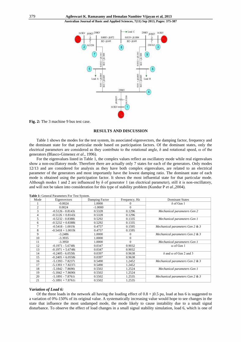
Therefore it will be more beneficial to look at the graph depicting all the parameters of the machines on the
network and their changes over this range. The plot is of the participation factor of each state in that particular
mode for a range of 0% to 150%.
Fig. 3: Plot of participation factors of 3 machine’s parameters in network for a 0% -150% increase in load 6
values.
The pattern of change exhibited by variation in loading is similar to that of variation in generation.
Although the influential state still remains to be rotational speed of, ω1 of machine 1, nevertheless it is
observable that an increase in participation of rotor angle, δ3 is significant. Partly because machine 1 is the slack
bus, its view on the system is generally constant. On the other hand, the sharp increase in participation of
machine 3's rotor angle, shows that it requires sufficient synchronizing torque.
Also, from the position of the load with reference to the generator, it can be theorized that the increase in
load affects the nearest located generator's parameters. In this case, an increase in load 6's properties, affects
both the rotor angle and rotational speed of machine 3, although the angle more than speed. Also, chances exits
that if the percent increase in load was more than 150%, the participation of rotor angle of machine 3 could
overstep the influence of rotational speed of machine 1 and become the higher risk at instability. Overall, it
appears that increasing the load affects the instability of the closest located generator.
381 Agileswari K. Ramasamy and Hemalan Nambier Vijayan et al, 2013
Australian Journal of Basic and Applied Sciences, 7(11) Sep 2013, Pages: 375-387
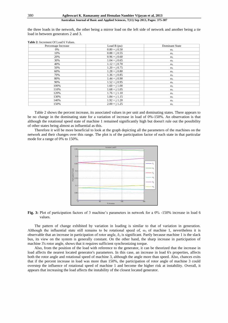
Fig. 4: Swinging at 0% increase in base loading of load 6.
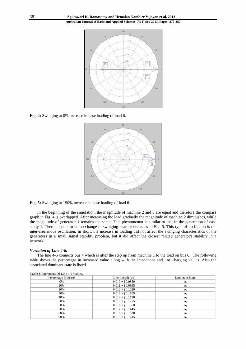
Fig. 5: Swinging at 150% increase in base loading of load 6.
In the beginning of the simulation, the magnitude of machine 2 and 3 are equal and therefore the compass
graph in Fig. 4 is overlapped. After increasing the load gradually the magnitude of machine 2 diminishes, while
the magnitude of generator 1 remains the same. This phenomenon is similar to that in the generation of case
study 1. There appears to be no change in swinging characteristics as in Fig. 5. This type of oscillation is the
inter-area mode oscillation. In short, the increase in loading did not affect the swinging characteristics of the
generators in a small signal stability problem, but it did affect the closest related generator's stability in a
network.
Variation of Line 4-6:
The line 4-6 connects bus 4 which is after the step up from machine 1 to the load on bus 6. The following
table shows the percentage in increased value along with the impedance and line charging values. Also the
associated dominant state is listed.
Table 3: Increment Of Line 4-6 Values.
Percentage Increase Line Length (pu) Dominant State
0% 0.010 + j 0.0850 ω1
10% 0.011 + j 0.0935 ω1
20% 0.012 + j 0.1020 ω1
30% 0.013 + j 0.1105 ω1
40% 0.014 + j 0.1190 ω1
50% 0.015 + j 0.1275 ω1
60% 0.016 + j 0.1360 ω1
70% 0.017 + j 0.1445 ω1
80% 0.018 + j 0.1530 ω1
90% 0.019 + j 0.1615 ω1

382 Agileswari K. Ramasamy and Hemalan Nambier Vijayan et al, 2013
Australian Journal of Basic and Applied Sciences, 7(11) Sep 2013, Pages: 375-387
100% 0.020 + j 0.1700 ω1
110% 0.021 + j 0.1785 δ3
120% 0.022 + j 0.1870 δ3
130% 0.023 + j 0.1955 δ3
140% 0.024 + j 0.2040 δ3
150% 0.025 + j 0.2125 δ3
From Table 3, there is a change in dominant states at 110% increase in line length of this particular line.
Again, machine 1 being the slack is not affected but the next closest machine would be machine 3.
Considerably, it takes some higher percentage in increase of line to actually cause the participation of rotor
angle of machine 3 to become most influential. This is likely that the physical distance of line 4-6 is farthest
from machine 3 and as expected, a higher amount of line difference would be needed to cause the prominence in
state of δ3.
Fig. 6: Plot of participation factors of 3 machine’s parameters in network for 0% -150% increase in line length
of line 4-6.
From Fig. 6, the increase of line shows an exponentially increase in participation of machine 3 states.
Unlike for generation and loading variation which increase almost linearly. This large change or increase in
participation reflects on the senility of the parameter with respect to stability of the system.
Generally, it is known that changes in line can have drastic effect on a particular network. Machine 2 and
machine 3 are corresponding oppositely which is similar as previously discussed as they are located on opposite
sides of the network. Also, it can be theorized that changes in a line would affect the nearest located generator in
terms of its synchronism with the network.
An instability resulting from rotor angle shows lack of sufficient synchronizing torque. A view of swinging
characteristic of this system is shown in the following figures.
Fig. 7: Swinging at 50% variation in line length of line 4-6.
383 Agileswari K. Ramasamy and Hemalan Nambier Vijayan et al, 2013
Australian Journal of Basic and Applied Sciences, 7(11) Sep 2013, Pages: 375-387
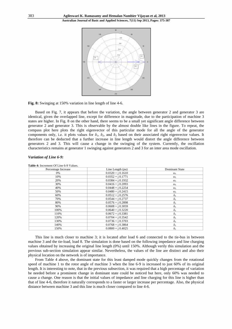
Fig. 8: Swinging at 150% variation in line length of line 4-6.
Based on Fig. 7, it appears that before the variation, the angle between generator 2 and generator 3 are
identical, given the overlapped line, except for difference in magnitude, due to the participation of machine 3
states are higher. In Fig. 8 on the other hand, there seems to be a small yet significant angle difference between
generator 2 and generator 3. This is observable by the almost double like lines in the figure. To repeat, the
compass plot here plots the right eigenvector of this particular mode for all the angle of the generator
components only, i.e. it plots values for δ1, δ2, and δ3 based on their associated right eigenvector values. It
therefore can be deducted that a further increase in line length would distort the angle difference between
generators 2 and 3. This will cause a change in the swinging of the system. Currently, the oscillation
characteristics remains at generator 1 swinging against generators 2 and 3 for an inter area mode oscillation.
Variation of Line 6-9:
Table 4: Increment Of Line 6-9 Values.
Percentage Increase Line Length (pu) Dominant State
0% 0.0320 + j 0.1610 ω1
10% 0.0352 + j 0.1771 ω1
20% 0.0384 + j 0.1932 ω1
30% 0.0416 + j 0.2093 ω1
40% 0.0448 + j 0.2254 ω1
50% 0.0480 + j 0.2415 ω1
60% 0.0512 + j 0.2576 δ3
70% 0.0544 + j 0.2737 δ3
80% 0.0576 + j 0.2898 δ3
90% 0.0608 + j 0.3059 δ3
100% 0.0640 + j 0.3220 δ3
110% 0.0672 + j 0.3381 δ3
120% 0.0704 + j 0.3542 δ3
130% 0.0736 + j 0.3703 δ3
140% 0.0768 + j 0.3864 δ3
150% 0.0800 + j 0.4025 δ3
This line is much closer to machine 3; it is located after load 6 and connected to the tie-bus in between
machine 3 and the tie-load, load 8. The simulation is done based on the following impedance and line charging
values obtained by increasing the original line length (0%) until 150%. Although verily this simulation and the
previous sub-section simulation appear similar. Nevertheless, the values of the line are distinct and also their
physical location on the network is of importance.
From Table 4 above, the dominant state for this least damped mode quickly changes from the rotational
speed of machine 1 to the rotor angle of machine 3 when the line 6-9 is increased to just 60% of its original
length. It is interesting to note, that in the previous subsection, it was required that a high percentage of variation
be needed before a prominent change in dominant state could be noticed but here, only 60% was needed to
cause a change. One reason is that the initial values of impedance and line charging for this line is higher than
that of line 4-6, therefore it naturally corresponds to a faster or larger increase per percentage. Also, the physical
distance between machine 3 and this line is much closer compared to line 4-6.
384 Agileswari K. Ramasamy and Hemalan Nambier Vijayan et al, 2013
Australian Journal of Basic and Applied Sciences, 7(11) Sep 2013, Pages: 375-387
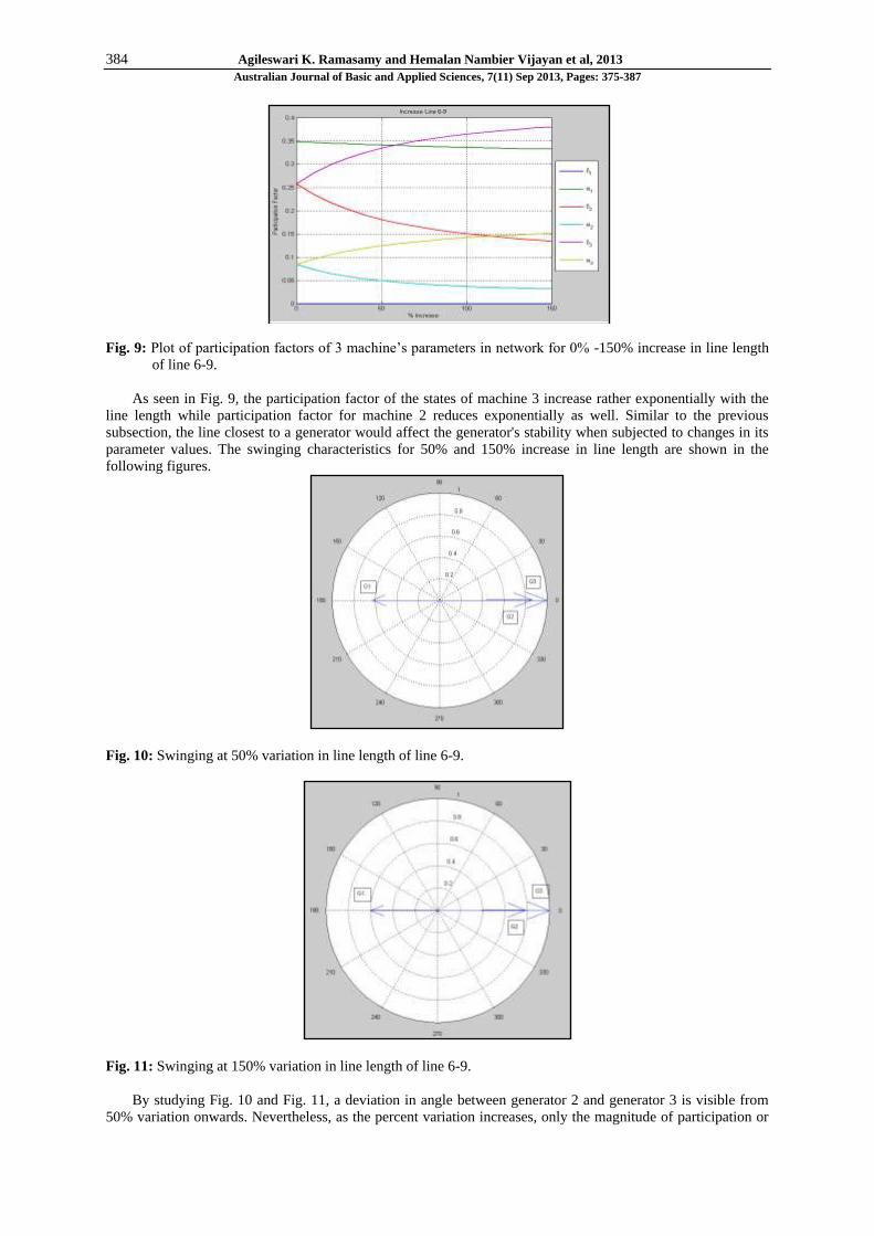
Fig. 9: Plot of participation factors of 3 machine’s parameters in network for 0% -150% increase in line length
of line 6-9.
As seen in Fig. 9, the participation factor of the states of machine 3 increase rather exponentially with the
line length while participation factor for machine 2 reduces exponentially as well. Similar to the previous
subsection, the line closest to a generator would affect the generator's stability when subjected to changes in its
parameter values. The swinging characteristics for 50% and 150% increase in line length are shown in the
following figures.
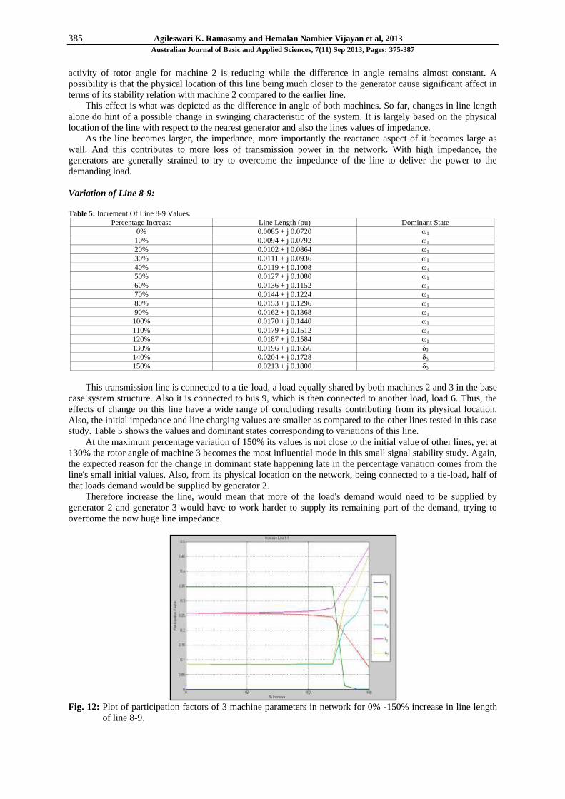
Fig. 10: Swinging at 50% variation in line length of line 6-9.
Fig. 11: Swinging at 150% variation in line length of line 6-9.
By studying Fig. 10 and Fig. 11, a deviation in angle between generator 2 and generator 3 is visible from
50% variation onwards. Nevertheless, as the percent variation increases, only the magnitude of participation or
385 Agileswari K. Ramasamy and Hemalan Nambier Vijayan et al, 2013
Australian Journal of Basic and Applied Sciences, 7(11) Sep 2013, Pages: 375-387
activity of rotor angle for machine 2 is reducing while the difference in angle remains almost constant. A
possibility is that the physical location of this line being much closer to the generator cause significant affect in
terms of its stability relation with machine 2 compared to the earlier line.
This effect is what was depicted as the difference in angle of both machines. So far, changes in line length
alone do hint of a possible change in swinging characteristic of the system. It is largely based on the physical
location of the line with respect to the nearest generator and also the lines values of impedance.
As the line becomes larger, the impedance, more importantly the reactance aspect of it becomes large as
well. And this contributes to more loss of transmission power in the network. With high impedance, the
generators are generally strained to try to overcome the impedance of the line to deliver the power to the
demanding load.
Variation of Line 8-9:
Table 5: Increment Of Line 8-9 Values.
Percentage Increase Line Length (pu) Dominant State
0% 0.0085 + j 0.0720 ω1
10% 0.0094 + j 0.0792 ω1
20% 0.0102 + j 0.0864 ω1
30% 0.0111 + j 0.0936 ω1
40% 0.0119 + j 0.1008 ω1
50% 0.0127 + j 0.1080 ω1
60% 0.0136 + j 0.1152 ω1
70% 0.0144 + j 0.1224 ω1
80% 0.0153 + j 0.1296 ω1
90% 0.0162 + j 0.1368 ω1
100% 0.0170 + j 0.1440 ω1
110% 0.0179 + j 0.1512 ω1
120% 0.0187 + j 0.1584 ω1
130% 0.0196 + j 0.1656 δ3
140% 0.0204 + j 0.1728 δ3
150% 0.0213 + j 0.1800 δ3
This transmission line is connected to a tie-load, a load equally shared by both machines 2 and 3 in the base
case system structure. Also it is connected to bus 9, which is then connected to another load, load 6. Thus, the
effects of change on this line have a wide range of concluding results contributing from its physical location.
Also, the initial impedance and line charging values are smaller as compared to the other lines tested in this case
study. Table 5 shows the values and dominant states corresponding to variations of this line.
At the maximum percentage variation of 150% its values is not close to the initial value of other lines, yet at
130% the rotor angle of machine 3 becomes the most influential mode in this small signal stability study. Again,
the expected reason for the change in dominant state happening late in the percentage variation comes from the
line's small initial values. Also, from its physical location on the network, being connected to a tie-load, half of
that loads demand would be supplied by generator 2.
Therefore increase the line, would mean that more of the load's demand would need to be supplied by
generator 2 and generator 3 would have to work harder to supply its remaining part of the demand, trying to
overcome the now huge line impedance.
Fig. 12: Plot of participation factors of 3 machine parameters in network for 0% -150% increase in line length
of line 8-9.
386 Agileswari K. Ramasamy and Hemalan Nambier Vijayan et al, 2013
Australian Journal of Basic and Applied Sciences, 7(11) Sep 2013, Pages: 375-387
The figure above shows a very unique response of increasing the line 8-9 on a range of 0% to 150%. From
0% to around 120% the graphs shows that participation factors of the system when subjected to small signal
stability disturbances responds as predicted from earlier case studies. Nevertheless, after 130% there is a
significant change in the participation characteristics. Firstly, after this point, the rotor angle of machine 3
becomes the most dominant state, which as discussed earlier is due to the fact that the modulation of line length
is closer to this generator then machine 2.
The uniqueness here appears at 130% where the lines respond very rapidly. The rotor angle for machine 2’s
response is inversed to machine 3’s as predicted in previous case studies. At 120% the participation factor of the
rotational speed of machine 1 drops rapidly to an almost zero value. This indicates the participation of machine
1 in this mode is almost nonexistent. This means that machine 1 is not at all a possibility for instability in this
condition.
A high participation factor would hint that a particular state was more likely to be the weak link, or possibly
failure point of the system network. Another interesting observation is the rotational speeds of machine 2 and
machine 3. In previous case studies, these parameters are always inversely proportional to each other;
nevertheless, here it is noticeable that both machines rotational speed seems to be increasing almost linearly as
the line is increased. Just as it was explained earlier, this is likely to be caused by the physical location of the
line, being connected to a tie-load (Guo Chunlin et al., 2002, Graham Rogers, 2000,L.L Grigsby, 2001).
The increase in line length of 8-9, would mean that load 8 then becomes networkly closer to machine 2 and
demands supply from it. In such a condition, it is logical for the participation of the state of machine 2 rotational
speed to increase as well. Comparing with the participation factor of rotational speed of machine 3 on the other
hand, it is still largely more influential, this, again, would be due to the line being closer to machine 3.
Fig. 13: Swinging at 50% variation in line length of line 8-9.
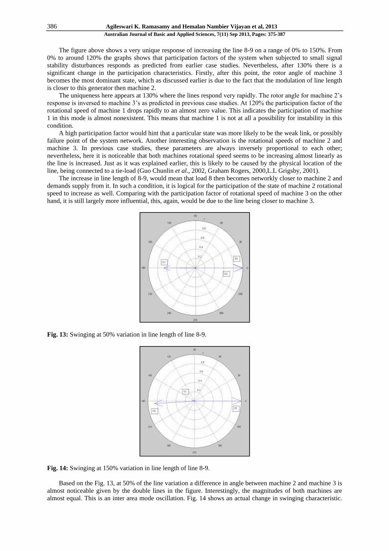
Fig. 14: Swinging at 150% variation in line length of line 8-9.
Based on the Fig. 13, at 50% of the line variation a difference in angle between machine 2 and machine 3 is
almost noticeable given by the double lines in the figure. Interestingly, the magnitudes of both machines are
almost equal. This is an inter area mode oscillation. Fig. 14 shows an actual change in swinging characteristic.

387 Agileswari K. Ramasamy and Hemalan Nambier Vijayan et al, 2013
Australian Journal of Basic and Applied Sciences, 7(11) Sep 2013, Pages: 375-387
Generator 2 and generator 1 are swinging against generator 3, although the participation of generator 1 is almost
zero. Relatively, both generators on the opposite sides of the network sharing the same load 8 are now swinging
against each other when the line 8-9 is extended to 150% its present value. Line length variations seem to have
more critical effect on stability then other parameters.
Conclusions:
Case studies were performed each for variations in loading capacity variations and also changes in line
lengths for three particular locations on the network. The variations were performed for an increase in initial
values for a range of 0%-150%. Simulations was analyzed by output data such as participation factors denoting
dominant states, least damped modes, right eigenvector for all machine rotor angle parameters - to detect
swinging characteristics, and participation factors of all machine states to observe trending features. It was
observed that increasing the generation output for a machine would affect its stability when subjected to a small
disturbance. Also, an increase in loading of a particular load would have related effects with the generation
closest to it on the physical network. Also line length changes effect the generator closest to it as well. In
addition, the physical location of lines and loads and other possibilities of instability with respect to a small
signal disturbance were discussed.
ACKNOWLEDGMENTS
This work was supported by The Ministry of Higher Education Malaysia (MOHE) via the FRGS
(Fundamental Research Grant Scheme) Grant 01090003 FRGS.
REFERENCES
Angelidis, G. and A. Semlyen, 1996. Improved Methodologies for the Calculation of Critical Eigenvalues
in Small Signal Stability Analysis. IEEE Trans. Power Syst., 11(3): 1209-1217.
Assessment of Large-Scale Power Systems. IEEE Trans. Power Syst., 10: 1979-1985.
Bezerra, L.H. and C. Tomei, 1999. Spectral Transformation Algorithms for Computing Unstable Modes,
Comp. Appl. Math., 18(1): 1-15.
Blasco-Gimenez et al., 1996. Dynamic Performance Limitations for MRAS Based Sensorless Induction
Motor.
Castrillon, N.J., X.M. S.A. E.S.P., Medellin, Colombia Colome, D.G., 2012. Small Signal Stability
Sensitivity to Generation Dispatch Through Participation Factor. Transmission and Distribution: Latin
America Conference and Exposition (T&D-LA), 2012 Sixth IEEE/PES, 3-5 September.
Cliffe, K.A., T.J. Garratt and A. Spence, 1994. Eigenvalues of Block Matrices Arising from Problems in
Fluid Mechanics. SIAM J. Matrix Anal.Appl.,15(4): 1310-1318.
Drives. Part 1: Stability Analysis for the Closed Loop Drives. IEE Proc. Electric Power Applications, 143:
113-122.
El-Amin, I.M., A. Al-Shehri, G. Opoku and S.A. Al-Baiyat, 1994. Electric Network Interconnection of
Mashreq Arab Countries. IEEE Power Engineering Review, 14(12): 26-28.
Graham Rogers, 2000. Power System Oscillations. Kluwer Academic Publishers, USA.
Grigsby, L.L., 2001. Power System Dynamics and Stability. The Electric Power Engineering Handbook.
CRC Press and IEEE Press.
Guo Chunlin, et al., 2002. Stability Control of TCSC between Interconnected Power Networks. IEEE
International: 1943-1946.
Hsu, Yuan-Yih et al., 1987. Identification of Optimum Location for Stabilizer Applications Using
Participation Factors. IEE Proceedings on Generation, Transmission and Distribution, 134: 238-244.
Kundur, P., et al., 2004. Definition and Classification of Power System Stability. IEEE Transactions On
Power Systems, 19: 1387-1401.
Kundur, P., M. Klien, G.J. Rogers and M.S. Zywno, 1989. Application of Power System Stabilizers for
Enchancement of Overall Stability. IEEE.Transc. on Power System, 4: 614-626.
Lima, L.T.G., L.H. Bezerra, C. Tomei and N. Martins, 1995. New Methods for Fast Small-Signal Stability
Ma, J., Z.Y. Dong and P. Zhang, 2006. Comparison of BR and QR Eigenvalue Algorithms for Power
System Small Signal Stability Analysis. IEEE Trans. Power Syst., 21(4): 1848-1855.
Makarov, Y.V., Z.Y. Dong and D.J. Hill, 1998. A General Method for Small Signal Stability Analysis.
IEEE Trans. Power Syst., 13: 1979-1985.
Meerbergen, K., A. Spence and D. Roose, 1994. Shift-invert and Cayley Transforms for Detection of
Rightmost Eigenvalues of Nonsymmetric Matrices. BIT, 34(3): 409-423.
Richard, G. Farmer, 2006. Power System Dynamics and Stability. Taylor & Francis Group, LLC.
Rodriguez, O., et al., 2007. A Comparative Analysis of Methodologies for the Representation of Nonlinear
Oscillations in Dynamic Systems. IEEE Lausanne Power Tech., 172-177.