slides.pdf
126
Hacia una lógica computacional cuántica Alejandro Díaz-Caro Université Paris-Ouest Nanterre La Défense & INRIA Paris-Roquencourt 23 avenue d’Italie, París FCEIA – UNR 9 de Agosto de 2013
-
Upload
alejandro-diaz-caro -
Category
Documents
-
view
212 -
download
0
Transcript of slides.pdf
Hacia una lógica computacional cuántica
Alejandro Díaz-CaroUniversité Paris-Ouest Nanterre La Défense
& INRIA Paris-Roquencourt23 avenue d’Italie, París
FCEIA – UNR9 de Agosto de 2013
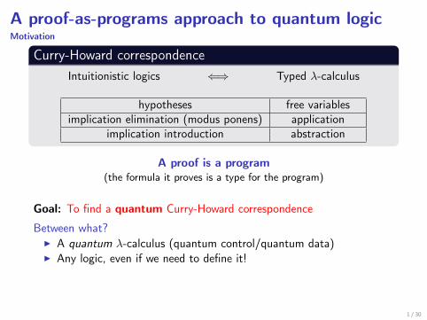
A proof-as-programs approach to quantum logicMotivation
Curry-Howard correspondenceIntuitionistic logics ⇐⇒ Typed λ-calculus
hypotheses free variablesimplication elimination (modus ponens) application
implication introduction abstraction
A proof is a program(the formula it proves is a type for the program)
Goal: To find a quantum Curry-Howard correspondence
Between what?I A quantum λ-calculus (quantum control/quantum data)I Any logic, even if we need to define it!
Computational quantum logicWe want a logic such that its proofs are quantum programs
1 / 30
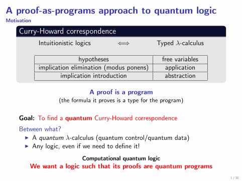
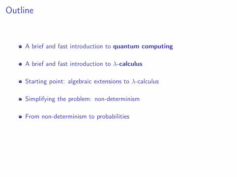
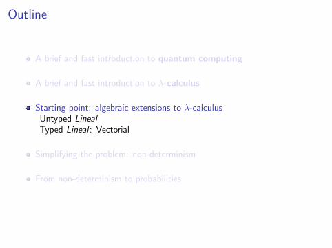
Outline
A brief and fast introduction to quantum computing
A brief and fast introduction to λ-calculus
Starting point: algebraic extensions to λ-calculus
Simplifying the problem: non-determinism
From non-determinism to probabilities
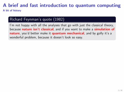
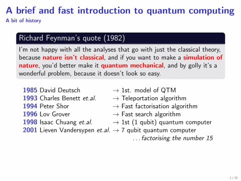
A brief and fast introduction to quantum computingA bit of history
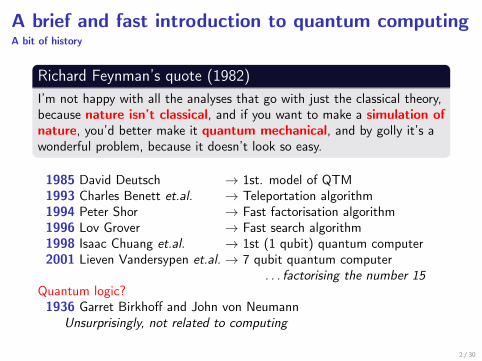
Richard Feynman’s quote (1982)I’m not happy with all the analyses that go with just the classical theory,because nature isn’t classical, and if you want to make a simulation ofnature, you’d better make it quantum mechanical, and by golly it’s awonderful problem, because it doesn’t look so easy.
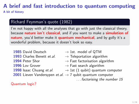
1985 David Deutsch → 1st. model of QTM1993 Charles Benett et.al. → Teleportation algorithm1994 Peter Shor → Fast factorisation algorithm1996 Lov Grover → Fast search algorithm1998 Isaac Chuang et.al. → 1st (1 qubit) quantum computer2001 Lieven Vandersypen et.al. → 7 qubit quantum computer
. . . factorising the number 15Quantum logic?1936 Garret Birkhoff and John von Neumann
Unsurprisingly, not related to computing
2 / 30

A brief and fast introduction to quantum computingA bit of history
Richard Feynman’s quote (1982)I’m not happy with all the analyses that go with just the classical theory,because nature isn’t classical, and if you want to make a simulation ofnature, you’d better make it quantum mechanical, and by golly it’s awonderful problem, because it doesn’t look so easy.
1985 David Deutsch → 1st. model of QTM1993 Charles Benett et.al. → Teleportation algorithm1994 Peter Shor → Fast factorisation algorithm1996 Lov Grover → Fast search algorithm1998 Isaac Chuang et.al. → 1st (1 qubit) quantum computer2001 Lieven Vandersypen et.al. → 7 qubit quantum computer
. . . factorising the number 15Quantum logic?1936 Garret Birkhoff and John von Neumann
Unsurprisingly, not related to computing
2 / 30
A brief and fast introduction to quantum computingA bit of history
Richard Feynman’s quote (1982)I’m not happy with all the analyses that go with just the classical theory,because nature isn’t classical, and if you want to make a simulation ofnature, you’d better make it quantum mechanical, and by golly it’s awonderful problem, because it doesn’t look so easy.
1985 David Deutsch → 1st. model of QTM1993 Charles Benett et.al. → Teleportation algorithm1994 Peter Shor → Fast factorisation algorithm1996 Lov Grover → Fast search algorithm1998 Isaac Chuang et.al. → 1st (1 qubit) quantum computer2001 Lieven Vandersypen et.al. → 7 qubit quantum computer
. . . factorising the number 15
Quantum logic?1936 Garret Birkhoff and John von Neumann
Unsurprisingly, not related to computing
2 / 30
A brief and fast introduction to quantum computingA bit of history
Richard Feynman’s quote (1982)I’m not happy with all the analyses that go with just the classical theory,because nature isn’t classical, and if you want to make a simulation ofnature, you’d better make it quantum mechanical, and by golly it’s awonderful problem, because it doesn’t look so easy.
1985 David Deutsch → 1st. model of QTM1993 Charles Benett et.al. → Teleportation algorithm1994 Peter Shor → Fast factorisation algorithm1996 Lov Grover → Fast search algorithm1998 Isaac Chuang et.al. → 1st (1 qubit) quantum computer2001 Lieven Vandersypen et.al. → 7 qubit quantum computer
. . . factorising the number 15Quantum logic?
1936 Garret Birkhoff and John von NeumannUnsurprisingly, not related to computing
2 / 30
A brief and fast introduction to quantum computingA bit of history
Richard Feynman’s quote (1982)I’m not happy with all the analyses that go with just the classical theory,because nature isn’t classical, and if you want to make a simulation ofnature, you’d better make it quantum mechanical, and by golly it’s awonderful problem, because it doesn’t look so easy.
1985 David Deutsch → 1st. model of QTM1993 Charles Benett et.al. → Teleportation algorithm1994 Peter Shor → Fast factorisation algorithm1996 Lov Grover → Fast search algorithm1998 Isaac Chuang et.al. → 1st (1 qubit) quantum computer2001 Lieven Vandersypen et.al. → 7 qubit quantum computer
. . . factorising the number 15Quantum logic?1936 Garret Birkhoff and John von Neumann
Unsurprisingly, not related to computing
2 / 30
A physics free introduction to quantum computingQuantum vs. Classic, side by side
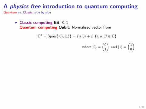
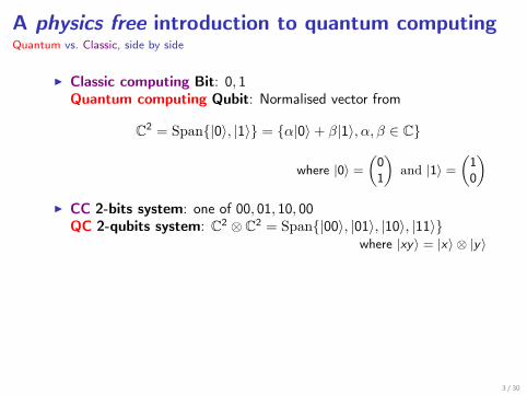
I Classic computing Bit: 0, 1Quantum computing Qubit: Normalised vector from
C2 = Span|0〉, |1〉 = α|0〉+ β|1〉, α, β ∈ C
where |0〉 =(
01
)and |1〉 =
(10
)
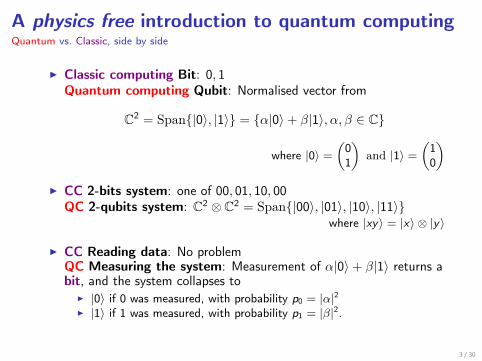
I CC 2-bits system: one of 00, 01, 10, 00QC 2-qubits system: C2 ⊗ C2 = Span|00〉, |01〉, |10〉, |11〉
where |xy〉 = |x〉 ⊗ |y〉
I CC Reading data: No problemQC Measuring the system: Measurement of α|0〉+ β|1〉 returns abit, and the system collapses to
I |0〉 if 0 was measured, with probability p0 = |α|2I |1〉 if 1 was measured, with probability p1 = |β|2.
3 / 30
A physics free introduction to quantum computingQuantum vs. Classic, side by side
I Classic computing Bit: 0, 1Quantum computing Qubit: Normalised vector from
C2 = Span|0〉, |1〉 = α|0〉+ β|1〉, α, β ∈ C
where |0〉 =(
01
)and |1〉 =
(10
)I CC 2-bits system: one of 00, 01, 10, 00
QC 2-qubits system: C2 ⊗ C2 = Span|00〉, |01〉, |10〉, |11〉where |xy〉 = |x〉 ⊗ |y〉
I CC Reading data: No problemQC Measuring the system: Measurement of α|0〉+ β|1〉 returns abit, and the system collapses to
I |0〉 if 0 was measured, with probability p0 = |α|2I |1〉 if 1 was measured, with probability p1 = |β|2.
3 / 30
A physics free introduction to quantum computingQuantum vs. Classic, side by side (cont.)
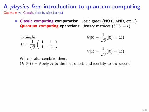
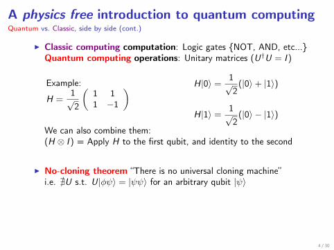
I Classic computing computation: Logic gates NOT, AND, etc...Quantum computing operations: Unitary matrices (U†U = I )
Example:
H =1√2
(1 11 −1
) H|0〉 =1√2
(|0〉+ |1〉)
H|1〉 =1√2
(|0〉 − |1〉)
We can also combine them:(H ⊗ I ) = Apply H to the first qubit, and identity to the second
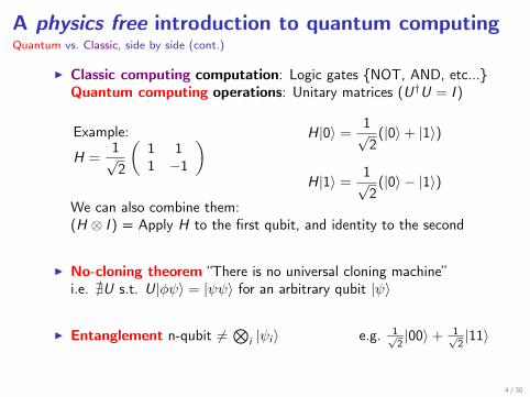
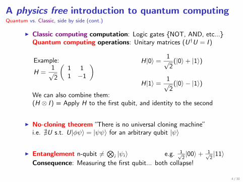
I No-cloning theorem “There is no universal cloning machine”i.e. @U s.t. U|φψ〉 = |ψψ〉 for an arbitrary qubit |ψ〉
I Entanglement n-qubit 6=⊗
i |ψi 〉 e.g. 1√2|00〉+ 1√
2|11〉
Consequence: Measuring the first qubit... both collapse!
4 / 30
A physics free introduction to quantum computingQuantum vs. Classic, side by side (cont.)
I Classic computing computation: Logic gates NOT, AND, etc...Quantum computing operations: Unitary matrices (U†U = I )
Example:
H =1√2
(1 11 −1
) H|0〉 =1√2
(|0〉+ |1〉)
H|1〉 =1√2
(|0〉 − |1〉)
We can also combine them:(H ⊗ I ) = Apply H to the first qubit, and identity to the second
I No-cloning theorem “There is no universal cloning machine”i.e. @U s.t. U|φψ〉 = |ψψ〉 for an arbitrary qubit |ψ〉
I Entanglement n-qubit 6=⊗
i |ψi 〉 e.g. 1√2|00〉+ 1√
2|11〉
Consequence: Measuring the first qubit... both collapse!
4 / 30
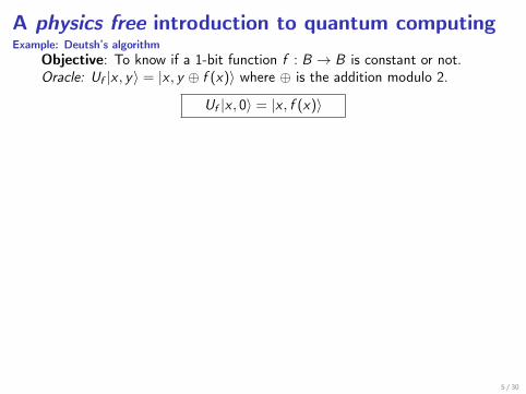
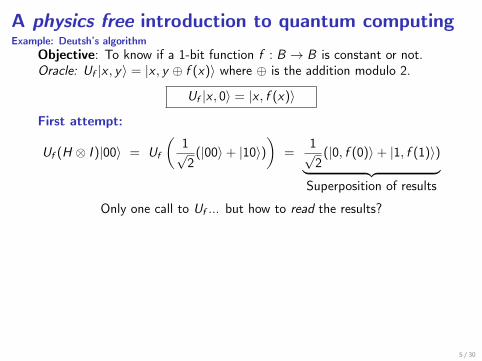
A physics free introduction to quantum computingExample: Deutsh’s algorithm
Objective: To know if a 1-bit function f : B → B is constant or not.Oracle: Uf |x , y〉 = |x , y ⊕ f (x)〉 where ⊕ is the addition modulo 2.
Uf |x , 0〉 = |x , f (x)〉
First attempt:
Uf (H ⊗ I )|00〉 = Uf
(1√2
(|00〉+ |10〉))
=1√2
(|0, f (0)〉+ |1, f (1)〉)︸ ︷︷ ︸Superposition of results
Only one call to Uf ... but how to read the results?
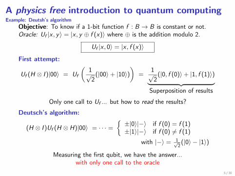
Deutsch’s algorithm:
(H ⊗ I )Uf (H ⊗ H)|00〉 = · · · =
±|0〉|−〉 if f (0) = f (1)±|1〉|−〉 if f (0) 6= f (1)
with |−〉 = 1√2
(|0〉 − |1〉)
Measuring the first qubit, we have the answer...with only one call to the oracle
5 / 30
A physics free introduction to quantum computingExample: Deutsh’s algorithm
Objective: To know if a 1-bit function f : B → B is constant or not.Oracle: Uf |x , y〉 = |x , y ⊕ f (x)〉 where ⊕ is the addition modulo 2.
Uf |x , 0〉 = |x , f (x)〉
First attempt:
Uf (H ⊗ I )|00〉 = Uf
(1√2
(|00〉+ |10〉))
=1√2
(|0, f (0)〉+ |1, f (1)〉)︸ ︷︷ ︸Superposition of results
Only one call to Uf ... but how to read the results?
Deutsch’s algorithm:
(H ⊗ I )Uf (H ⊗ H)|00〉 = · · · =
±|0〉|−〉 if f (0) = f (1)±|1〉|−〉 if f (0) 6= f (1)
with |−〉 = 1√2
(|0〉 − |1〉)
Measuring the first qubit, we have the answer...with only one call to the oracle
5 / 30
Outline
A brief and fast introduction to quantum computing
A brief and fast introduction to λ-calculusA brief and fast introduction to typed λ-calculusHow does it relates to intuitionistic logic?
Starting point: algebraic extensions to λ-calculus
Simplifying the problem: non-determinism
From non-determinism to probabilities
A brief and fast introduction to λ-calculusHistory and intuitions
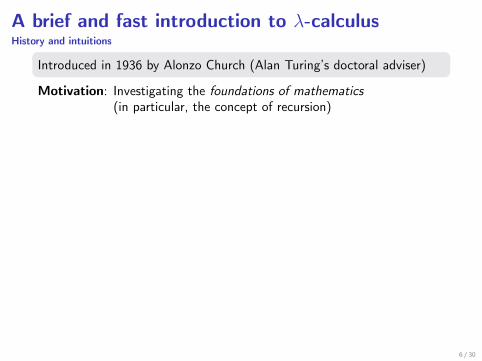
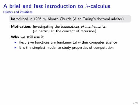
Introduced in 1936 by Alonzo Church (Alan Turing’s doctoral adviser)
Motivation: Investigating the foundations of mathematics(in particular, the concept of recursion)
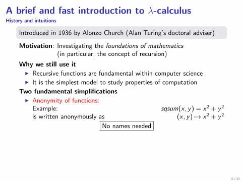
Why we still use itI Recursive functions are fundamental within computer scienceI It is the simplest model to study properties of computation
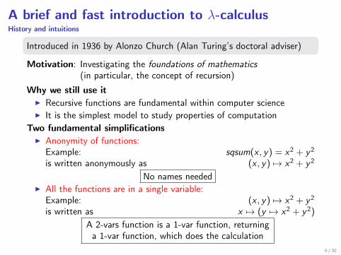
Two fundamental simplificationsI Anonymity of functions:
Example: sqsum(x , y) = x2 + y2
is written anonymously as (x , y) 7→ x2 + y2
No names neededI All the functions are in a single variable:
Example: (x , y) 7→ x2 + y2
is written as x 7→ (y 7→ x2 + y2)
A 2-vars function is a 1-var function, returninga 1-var function, which does the calculation
6 / 30
A brief and fast introduction to λ-calculusHistory and intuitions
Introduced in 1936 by Alonzo Church (Alan Turing’s doctoral adviser)
Motivation: Investigating the foundations of mathematics(in particular, the concept of recursion)
Why we still use itI Recursive functions are fundamental within computer scienceI It is the simplest model to study properties of computation
Two fundamental simplificationsI Anonymity of functions:
Example: sqsum(x , y) = x2 + y2
is written anonymously as (x , y) 7→ x2 + y2
No names needed
I All the functions are in a single variable:Example: (x , y) 7→ x2 + y2
is written as x 7→ (y 7→ x2 + y2)
A 2-vars function is a 1-var function, returninga 1-var function, which does the calculation
6 / 30
A brief and fast introduction to λ-calculusHistory and intuitions
Introduced in 1936 by Alonzo Church (Alan Turing’s doctoral adviser)
Motivation: Investigating the foundations of mathematics(in particular, the concept of recursion)
Why we still use itI Recursive functions are fundamental within computer scienceI It is the simplest model to study properties of computation
Two fundamental simplificationsI Anonymity of functions:
Example: sqsum(x , y) = x2 + y2
is written anonymously as (x , y) 7→ x2 + y2
No names neededI All the functions are in a single variable:
Example: (x , y) 7→ x2 + y2
is written as x 7→ (y 7→ x2 + y2)
A 2-vars function is a 1-var function, returninga 1-var function, which does the calculation
6 / 30
A brief and fast introduction to λ-calculusFormalisation
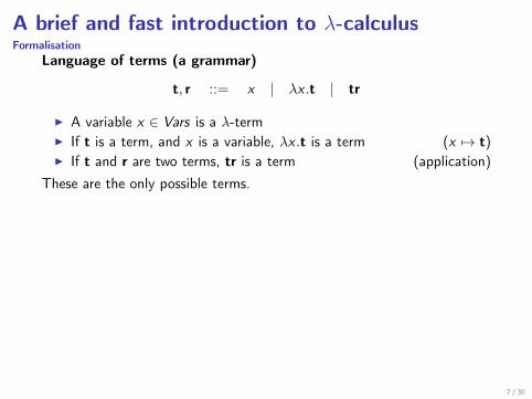
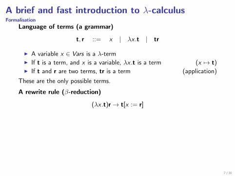
Language of terms (a grammar)
t, r ::= x | λx .t | tr
I A variable x ∈ Vars is a λ-termI If t is a term, and x is a variable, λx .t is a term (x 7→ t)I If t and r are two terms, tr is a term (application)
These are the only possible terms.
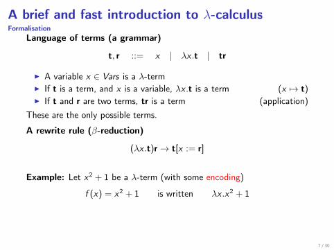
A rewrite rule (β-reduction)
(λx .t)r→ t[x := r]
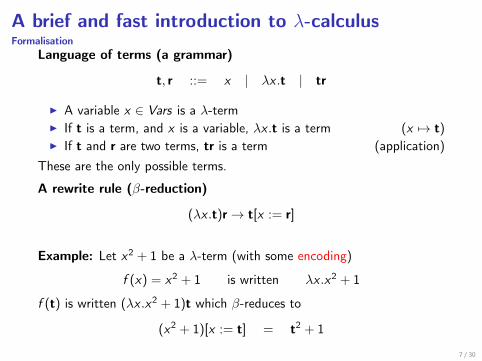
Example: Let x2 + 1 be a λ-term (with some encoding)
f (x) = x2 + 1 is written λx .x2 + 1
f (t) is written (λx .x2 + 1)t which β-reduces to
(x2 + 1)[x := t] = t2 + 1
7 / 30
A brief and fast introduction to λ-calculusFormalisation
Language of terms (a grammar)
t, r ::= x | λx .t | tr
I A variable x ∈ Vars is a λ-termI If t is a term, and x is a variable, λx .t is a term (x 7→ t)I If t and r are two terms, tr is a term (application)
These are the only possible terms.
A rewrite rule (β-reduction)
(λx .t)r→ t[x := r]
Example: Let x2 + 1 be a λ-term (with some encoding)
f (x) = x2 + 1 is written λx .x2 + 1
f (t) is written (λx .x2 + 1)t which β-reduces to
(x2 + 1)[x := t] = t2 + 1
7 / 30
A brief and fast introduction to λ-calculusNormal form
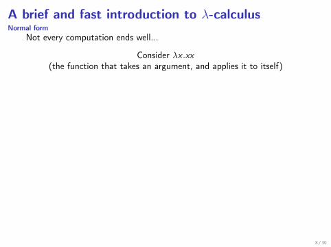
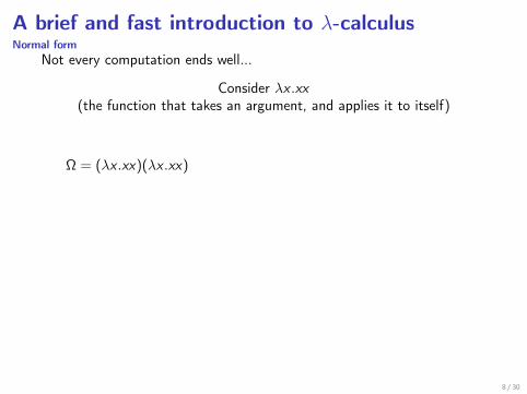
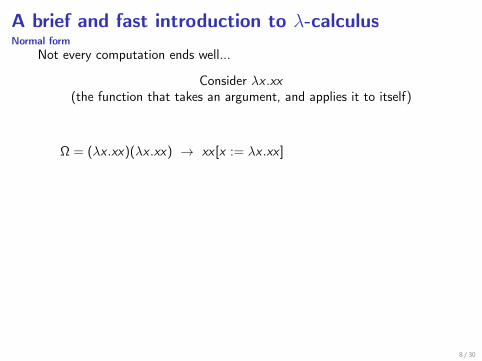
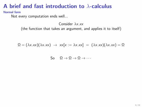
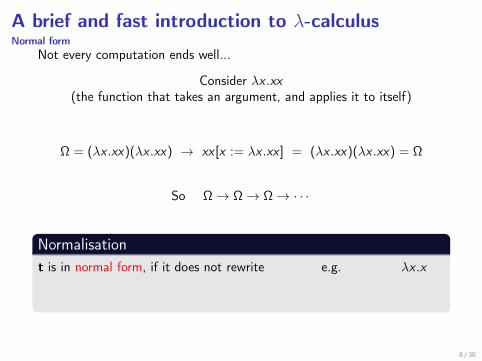
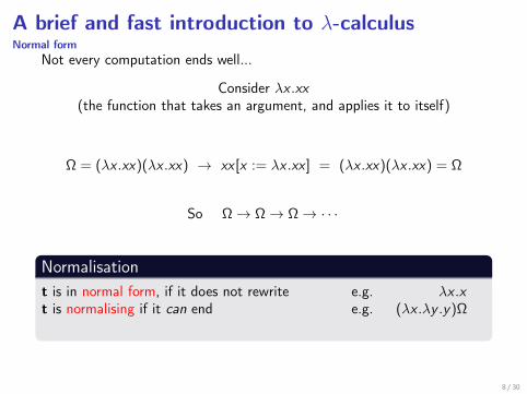
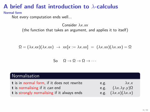
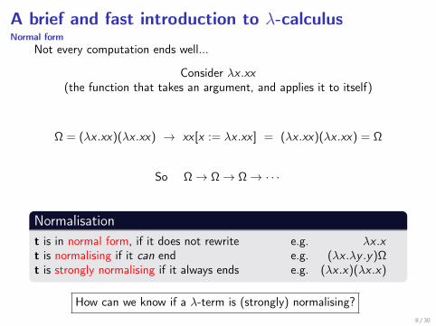
Not every computation ends well...
Consider λx .xx(the function that takes an argument, and applies it to itself)
Ω = (λx .xx)(λx .xx) → xx [x := λx .xx ] = (λx .xx)(λx .xx) = Ω
So Ω→ Ω→ Ω→ · · ·
Normalisationt is in normal form, if it does not rewrite e.g. λx .xt is normalising if it can end e.g. (λx .λy .y)Ωt is strongly normalising if it always ends e.g. (λx .x)(λx .x)
How can we know if a λ-term is (strongly) normalising?
8 / 30
A brief and fast introduction to λ-calculusNormal form
Not every computation ends well...
Consider λx .xx(the function that takes an argument, and applies it to itself)
Ω = (λx .xx)(λx .xx)
→ xx [x := λx .xx ] = (λx .xx)(λx .xx) = Ω
So Ω→ Ω→ Ω→ · · ·
Normalisationt is in normal form, if it does not rewrite e.g. λx .xt is normalising if it can end e.g. (λx .λy .y)Ωt is strongly normalising if it always ends e.g. (λx .x)(λx .x)
How can we know if a λ-term is (strongly) normalising?
8 / 30
A brief and fast introduction to λ-calculusNormal form
Not every computation ends well...
Consider λx .xx(the function that takes an argument, and applies it to itself)
Ω = (λx .xx)(λx .xx) → xx [x := λx .xx ]
= (λx .xx)(λx .xx) = Ω
So Ω→ Ω→ Ω→ · · ·
Normalisationt is in normal form, if it does not rewrite e.g. λx .xt is normalising if it can end e.g. (λx .λy .y)Ωt is strongly normalising if it always ends e.g. (λx .x)(λx .x)
How can we know if a λ-term is (strongly) normalising?
8 / 30
A brief and fast introduction to λ-calculusNormal form
Not every computation ends well...
Consider λx .xx(the function that takes an argument, and applies it to itself)
Ω = (λx .xx)(λx .xx) → xx [x := λx .xx ] = (λx .xx)(λx .xx) = Ω
So Ω→ Ω→ Ω→ · · ·
Normalisationt is in normal form, if it does not rewrite e.g. λx .xt is normalising if it can end e.g. (λx .λy .y)Ωt is strongly normalising if it always ends e.g. (λx .x)(λx .x)
How can we know if a λ-term is (strongly) normalising?
8 / 30
A brief and fast introduction to λ-calculusNormal form
Not every computation ends well...
Consider λx .xx(the function that takes an argument, and applies it to itself)
Ω = (λx .xx)(λx .xx) → xx [x := λx .xx ] = (λx .xx)(λx .xx) = Ω
So Ω→ Ω→ Ω→ · · ·
Normalisationt is in normal form, if it does not rewrite e.g. λx .x
t is normalising if it can end e.g. (λx .λy .y)Ωt is strongly normalising if it always ends e.g. (λx .x)(λx .x)
How can we know if a λ-term is (strongly) normalising?
8 / 30
A brief and fast introduction to λ-calculusNormal form
Not every computation ends well...
Consider λx .xx(the function that takes an argument, and applies it to itself)
Ω = (λx .xx)(λx .xx) → xx [x := λx .xx ] = (λx .xx)(λx .xx) = Ω
So Ω→ Ω→ Ω→ · · ·
Normalisationt is in normal form, if it does not rewrite e.g. λx .xt is normalising if it can end e.g. (λx .λy .y)Ω
t is strongly normalising if it always ends e.g. (λx .x)(λx .x)
How can we know if a λ-term is (strongly) normalising?
8 / 30
A brief and fast introduction to λ-calculusNormal form
Not every computation ends well...
Consider λx .xx(the function that takes an argument, and applies it to itself)
Ω = (λx .xx)(λx .xx) → xx [x := λx .xx ] = (λx .xx)(λx .xx) = Ω
So Ω→ Ω→ Ω→ · · ·
Normalisationt is in normal form, if it does not rewrite e.g. λx .xt is normalising if it can end e.g. (λx .λy .y)Ωt is strongly normalising if it always ends e.g. (λx .x)(λx .x)
How can we know if a λ-term is (strongly) normalising?
8 / 30
A brief and fast introduction to λ-calculusNormal form
Not every computation ends well...
Consider λx .xx(the function that takes an argument, and applies it to itself)
Ω = (λx .xx)(λx .xx) → xx [x := λx .xx ] = (λx .xx)(λx .xx) = Ω
So Ω→ Ω→ Ω→ · · ·
Normalisationt is in normal form, if it does not rewrite e.g. λx .xt is normalising if it can end e.g. (λx .λy .y)Ωt is strongly normalising if it always ends e.g. (λx .x)(λx .x)
How can we know if a λ-term is (strongly) normalising?8 / 30
A brief and fast introduction to typed λ-calculusSimply types
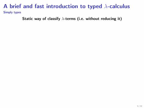
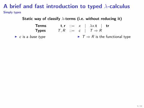
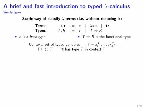
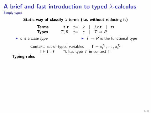
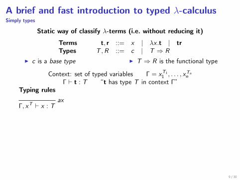
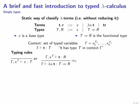
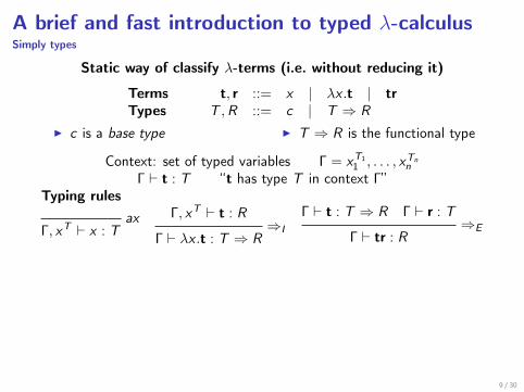
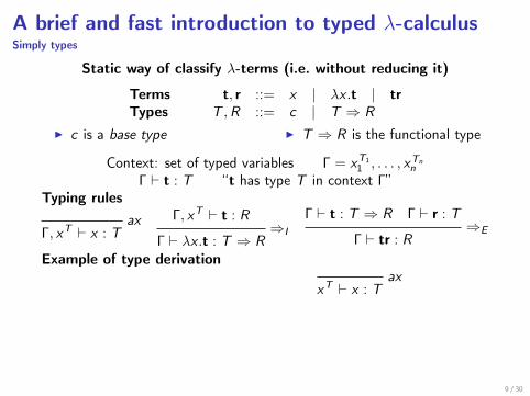
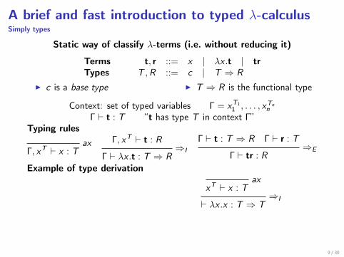
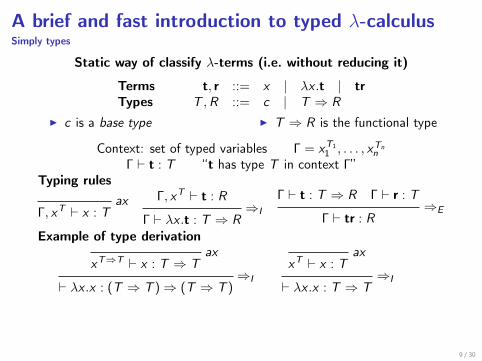
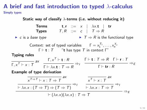
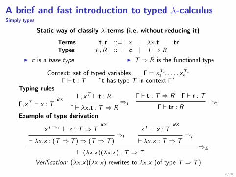
Static way of classify λ-terms (i.e. without reducing it)
Terms t, r ::= x | λx .t | trTypes T ,R ::= c | T ⇒ R
I c is a base type I T ⇒ R is the functional type
Context: set of typed variables Γ = xT11 , . . . , xTn
nΓ ` t : T “t has type T in context Γ”
Typing rulesax
Γ, xT ` x : TΓ, xT ` t : R
⇒IΓ ` λx .t : T ⇒ R
Γ ` t : T ⇒ R Γ ` r : T⇒E
Γ ` tr : RExample of type derivation
axxT⇒T ` x : T ⇒ T
⇒I` λx .x : (T ⇒ T )⇒ (T ⇒ T )
axxT ` x : T
⇒I` λx .x : T ⇒ T
⇒E` (λx .x)(λx .x) : T ⇒ T
Verification: (λx .x)(λx .x) rewrites to λx .x (of type T ⇒ T )
9 / 30
A brief and fast introduction to typed λ-calculusSimply types
Static way of classify λ-terms (i.e. without reducing it)
Terms t, r ::= x | λx .t | trTypes T ,R ::= c | T ⇒ R
I c is a base type I T ⇒ R is the functional type
Context: set of typed variables Γ = xT11 , . . . , xTn
nΓ ` t : T “t has type T in context Γ”
Typing rules
axΓ, xT ` x : T
Γ, xT ` t : R⇒I
Γ ` λx .t : T ⇒ R
Γ ` t : T ⇒ R Γ ` r : T⇒E
Γ ` tr : RExample of type derivation
axxT⇒T ` x : T ⇒ T
⇒I` λx .x : (T ⇒ T )⇒ (T ⇒ T )
axxT ` x : T
⇒I` λx .x : T ⇒ T
⇒E` (λx .x)(λx .x) : T ⇒ T
Verification: (λx .x)(λx .x) rewrites to λx .x (of type T ⇒ T )
9 / 30
A brief and fast introduction to typed λ-calculusSimply types
Static way of classify λ-terms (i.e. without reducing it)
Terms t, r ::= x | λx .t | trTypes T ,R ::= c | T ⇒ R
I c is a base type I T ⇒ R is the functional type
Context: set of typed variables Γ = xT11 , . . . , xTn
nΓ ` t : T “t has type T in context Γ”
Typing rulesax
Γ, xT ` x : T
Γ, xT ` t : R⇒I
Γ ` λx .t : T ⇒ R
Γ ` t : T ⇒ R Γ ` r : T⇒E
Γ ` tr : RExample of type derivation
axxT⇒T ` x : T ⇒ T
⇒I` λx .x : (T ⇒ T )⇒ (T ⇒ T )
axxT ` x : T
⇒I` λx .x : T ⇒ T
⇒E` (λx .x)(λx .x) : T ⇒ T
Verification: (λx .x)(λx .x) rewrites to λx .x (of type T ⇒ T )
9 / 30
A brief and fast introduction to typed λ-calculusSimply types
Static way of classify λ-terms (i.e. without reducing it)
Terms t, r ::= x | λx .t | trTypes T ,R ::= c | T ⇒ R
I c is a base type I T ⇒ R is the functional type
Context: set of typed variables Γ = xT11 , . . . , xTn
nΓ ` t : T “t has type T in context Γ”
Typing rulesax
Γ, xT ` x : TΓ, xT ` t : R
⇒IΓ ` λx .t : T ⇒ R
Γ ` t : T ⇒ R Γ ` r : T⇒E
Γ ` tr : RExample of type derivation
axxT⇒T ` x : T ⇒ T
⇒I` λx .x : (T ⇒ T )⇒ (T ⇒ T )
axxT ` x : T
⇒I` λx .x : T ⇒ T
⇒E` (λx .x)(λx .x) : T ⇒ T
Verification: (λx .x)(λx .x) rewrites to λx .x (of type T ⇒ T )
9 / 30
A brief and fast introduction to typed λ-calculusSimply types
Static way of classify λ-terms (i.e. without reducing it)
Terms t, r ::= x | λx .t | trTypes T ,R ::= c | T ⇒ R
I c is a base type I T ⇒ R is the functional type
Context: set of typed variables Γ = xT11 , . . . , xTn
nΓ ` t : T “t has type T in context Γ”
Typing rulesax
Γ, xT ` x : TΓ, xT ` t : R
⇒IΓ ` λx .t : T ⇒ R
Γ ` t : T ⇒ R Γ ` r : T⇒E
Γ ` tr : R
Example of type derivation
axxT⇒T ` x : T ⇒ T
⇒I` λx .x : (T ⇒ T )⇒ (T ⇒ T )
axxT ` x : T
⇒I` λx .x : T ⇒ T
⇒E` (λx .x)(λx .x) : T ⇒ T
Verification: (λx .x)(λx .x) rewrites to λx .x (of type T ⇒ T )
9 / 30
A brief and fast introduction to typed λ-calculusSimply types
Static way of classify λ-terms (i.e. without reducing it)
Terms t, r ::= x | λx .t | trTypes T ,R ::= c | T ⇒ R
I c is a base type I T ⇒ R is the functional type
Context: set of typed variables Γ = xT11 , . . . , xTn
nΓ ` t : T “t has type T in context Γ”
Typing rulesax
Γ, xT ` x : TΓ, xT ` t : R
⇒IΓ ` λx .t : T ⇒ R
Γ ` t : T ⇒ R Γ ` r : T⇒E
Γ ` tr : RExample of type derivation
axxT⇒T ` x : T ⇒ T
⇒I` λx .x : (T ⇒ T )⇒ (T ⇒ T )
axxT ` x : T
⇒I` λx .x : T ⇒ T
⇒E` (λx .x)(λx .x) : T ⇒ T
Verification: (λx .x)(λx .x) rewrites to λx .x (of type T ⇒ T )
9 / 30
A brief and fast introduction to typed λ-calculusSimply types
Static way of classify λ-terms (i.e. without reducing it)
Terms t, r ::= x | λx .t | trTypes T ,R ::= c | T ⇒ R
I c is a base type I T ⇒ R is the functional type
Context: set of typed variables Γ = xT11 , . . . , xTn
nΓ ` t : T “t has type T in context Γ”
Typing rulesax
Γ, xT ` x : TΓ, xT ` t : R
⇒IΓ ` λx .t : T ⇒ R
Γ ` t : T ⇒ R Γ ` r : T⇒E
Γ ` tr : RExample of type derivation
axxT⇒T ` x : T ⇒ T
⇒I` λx .x : (T ⇒ T )⇒ (T ⇒ T )
axxT ` x : T
⇒I` λx .x : T ⇒ T
⇒E` (λx .x)(λx .x) : T ⇒ T
Verification: (λx .x)(λx .x) rewrites to λx .x (of type T ⇒ T )
9 / 30
A brief and fast introduction to typed λ-calculusNormalisation
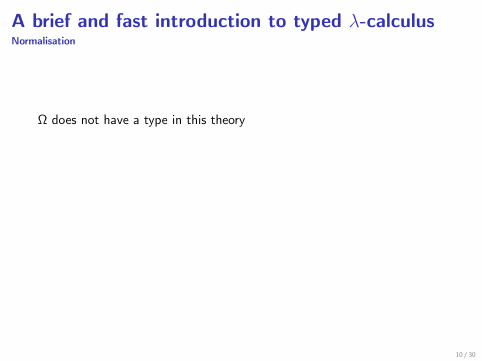
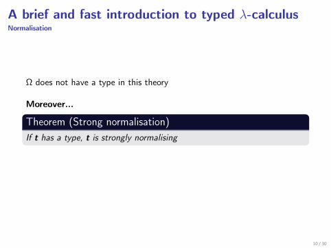
Ω does not have a type in this theory
Moreover...
Theorem (Strong normalisation)If t has a type, t is strongly normalising
Slogan “Well-typed programs cannot go wrong” — [R. Milner’78]
10 / 30
A brief and fast introduction to typed λ-calculusNormalisation
Ω does not have a type in this theory
Moreover...
Theorem (Strong normalisation)If t has a type, t is strongly normalising
Slogan “Well-typed programs cannot go wrong” — [R. Milner’78]
10 / 30

A brief and fast introduction to typed λ-calculusNormalisation
Ω does not have a type in this theory
Moreover...
Theorem (Strong normalisation)If t has a type, t is strongly normalising
Slogan “Well-typed programs cannot go wrong” — [R. Milner’78]
10 / 30
How does it relates to intuitionistic logics?A word on the Curry-Howard correspondence
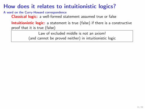
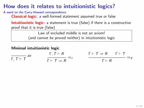
Classical logic: a well-formed statement assumed true or false
Intuitionistic logic: a statement is true (false) if there is a constructiveproof that it is true (false)
Law of excluded middle is not an axiom!(and cannot be proved neither) in intuitionistic logic
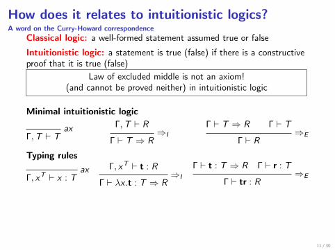
Minimal intuitionistic logic
axΓ,T ` T
Γ,T ` R⇒I
Γ ` T ⇒ R
Γ ` T ⇒ R Γ ` T⇒E
Γ ` R
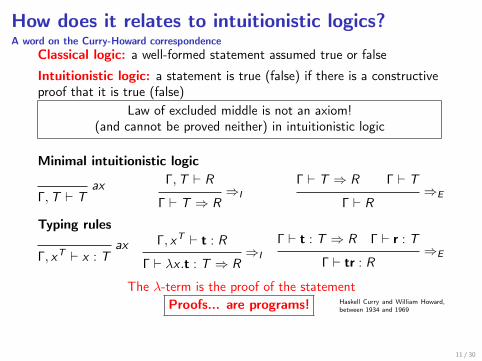
Typing rulesax
Γ, xT ` x : TΓ, xT ` t : R
⇒IΓ ` λx .t : T ⇒ R
Γ ` t : T ⇒ R Γ ` r : T⇒E
Γ ` tr : R
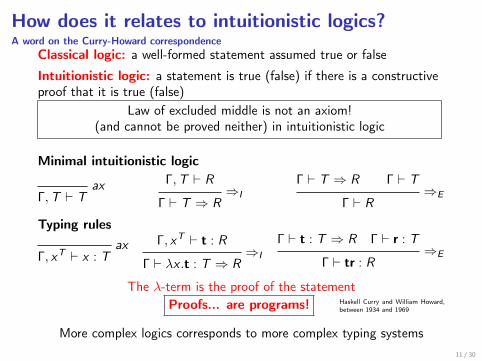
The λ-term is the proof of the statementProofs... are programs! Haskell Curry and William Howard,
between 1934 and 1969
More complex logics corresponds to more complex typing systems
11 / 30
How does it relates to intuitionistic logics?A word on the Curry-Howard correspondence
Classical logic: a well-formed statement assumed true or false
Intuitionistic logic: a statement is true (false) if there is a constructiveproof that it is true (false)
Law of excluded middle is not an axiom!(and cannot be proved neither) in intuitionistic logic
Minimal intuitionistic logic
axΓ,T ` T
Γ,T ` R⇒I
Γ ` T ⇒ R
Γ ` T ⇒ R Γ ` T⇒E
Γ ` R
Typing rulesax
Γ, xT ` x : TΓ, xT ` t : R
⇒IΓ ` λx .t : T ⇒ R
Γ ` t : T ⇒ R Γ ` r : T⇒E
Γ ` tr : R
The λ-term is the proof of the statementProofs... are programs! Haskell Curry and William Howard,
between 1934 and 1969
More complex logics corresponds to more complex typing systems11 / 30
Outline
A brief and fast introduction to quantum computing
A brief and fast introduction to λ-calculus
Starting point: algebraic extensions to λ-calculusUntyped LinealTyped Lineal : Vectorial
Simplifying the problem: non-determinism
From non-determinism to probabilities
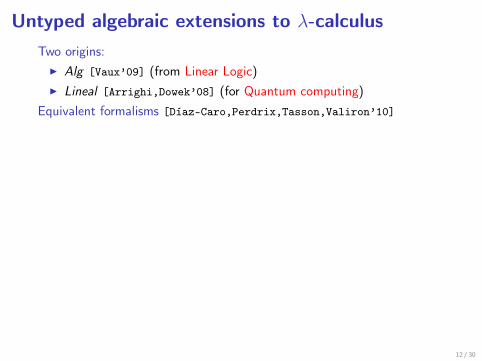
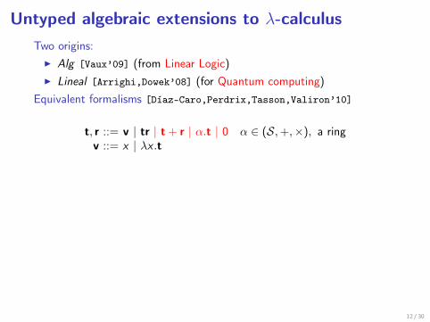
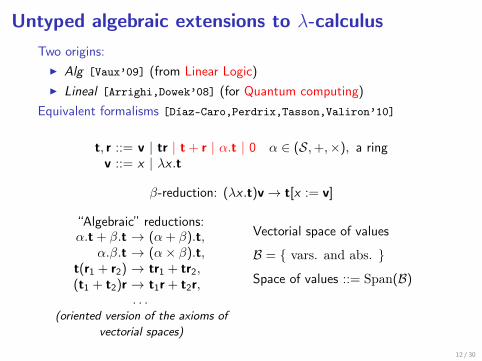
Untyped algebraic extensions to λ-calculusTwo origins:I Alg [Vaux’09] (from Linear Logic)I Lineal [Arrighi,Dowek’08] (for Quantum computing)
Equivalent formalisms [Díaz-Caro,Perdrix,Tasson,Valiron’10]
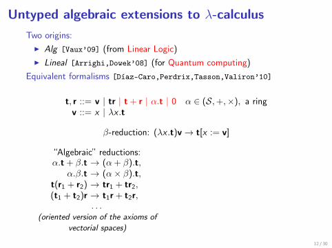
t, r ::= v | tr | t + r | α.t | 0 α ∈ (S,+,×), a ringv ::= x | λx .t
β-reduction: (λx .t)v→ t[x := v]
“Algebraic” reductions:α.t + β.t → (α + β).t,
α.β.t → (α× β).t,t(r1 + r2) → tr1 + tr2,(t1 + t2)r → t1r + t2r,
. . .(oriented version of the axioms of
vectorial spaces)
Vectorial space of values
B = vars. and abs.
Space of values ::= Span(B)
12 / 30
Untyped algebraic extensions to λ-calculusTwo origins:I Alg [Vaux’09] (from Linear Logic)I Lineal [Arrighi,Dowek’08] (for Quantum computing)
Equivalent formalisms [Díaz-Caro,Perdrix,Tasson,Valiron’10]
t, r ::= v | tr | t + r | α.t | 0 α ∈ (S,+,×), a ringv ::= x | λx .t
β-reduction: (λx .t)v→ t[x := v]
“Algebraic” reductions:α.t + β.t → (α + β).t,
α.β.t → (α× β).t,t(r1 + r2) → tr1 + tr2,(t1 + t2)r → t1r + t2r,
. . .(oriented version of the axioms of
vectorial spaces)
Vectorial space of values
B = vars. and abs.
Space of values ::= Span(B)
12 / 30
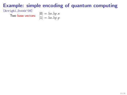
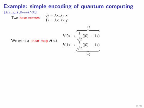
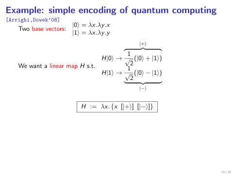
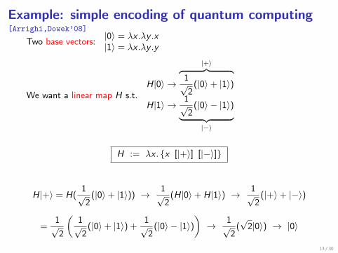
Example: simple encoding of quantum computing[Arrighi,Dowek’08]
Two base vectors: |0〉 = λx .λy .x|1〉 = λx .λy .y
We want a linear map H s.t.H|0〉 →
|+〉︷ ︸︸ ︷1√2
(|0〉+ |1〉)
H|1〉 → 1√2
(|0〉 − |1〉)︸ ︷︷ ︸|−〉
H := λx . x [|+〉] [|−〉]
H|+〉 = H(1√2
(|0〉+ |1〉)) → 1√2
(H|0〉+ H|1〉) → 1√2
(|+〉+ |−〉)
=1√2
(1√2
(|0〉+ |1〉) +1√2
(|0〉 − |1〉))→ 1√
2(√2|0〉) → |0〉
13 / 30
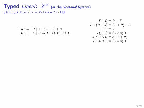
Typed Lineal : λvec (or the Vectorial System)[Arrighi,Díaz-Caro,Valiron’12–13]
T ,R ::= U | X | α.T | T + RU ::= X | U → T | ∀X.U | ∀X.U
T + R ≡ R + TT + (R + S) ≡ (T + R) + S
1.T ≡ Tα.(β.T ) ≡ (α× β).T
α.T + α.R ≡ α.(T + R)α.T + β.T ≡ (α + β).T
Most important property of λvec
` t :∑
i αi .Ti ⇒ t→∗∑
i αi .rit→∗
∑i αi .ri ⇒ ` t :
∑i αi .Ti + 0.R
where ` ri : Ti
A type system capturing the “vectorial” structure of terms. . . able to type matrices and vectors. . . able to check for probability distributions. . . or whatever application needing the structure of the vector
14 / 30
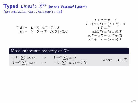
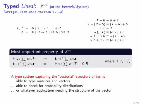
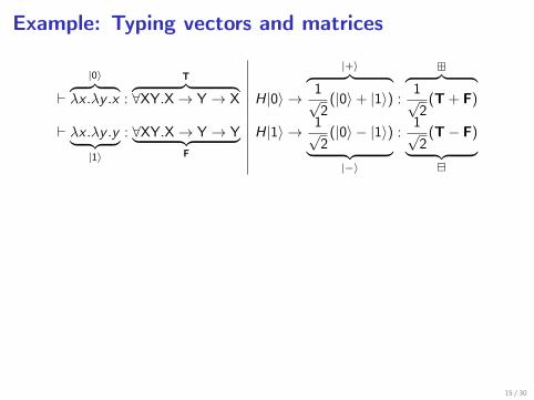
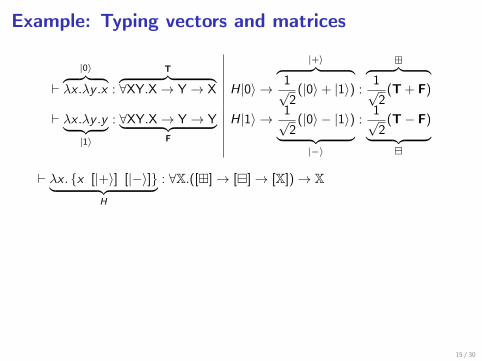
Example: Typing vectors and matrices
`|0〉︷ ︸︸ ︷
λx .λy .x :
T︷ ︸︸ ︷∀XY.X→ Y → X H|0〉 →
|+〉︷ ︸︸ ︷1√2
(|0〉+ |1〉) :
︷ ︸︸ ︷1√2
(T + F)
` λx .λy .y︸ ︷︷ ︸|1〉
: ∀XY.X→ Y → Y︸ ︷︷ ︸F
H|1〉 → 1√2
(|0〉 − |1〉)︸ ︷︷ ︸|−〉
:1√2
(T− F)︸ ︷︷ ︸
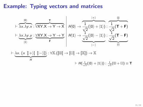
` λx . x [|+〉] [|−〉]︸ ︷︷ ︸H
: ∀X.([]→ []→ [X])→ X
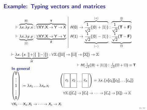
` H( 1√2(|0〉+ |1〉)) : 1√
2(+) ≡ T
In general0...1...0
:= λx1 . . . λxn.xi
c1 c2 . . . cn
= λx .x [c1][c2] . . . [cn]
∀X.([C1]→ [C2]→ · · · → [Cn]→ [X])→ X
∀X1 · · ·Xn.X1 → · · · → Xn → Xi
15 / 30
Example: Typing vectors and matrices
`|0〉︷ ︸︸ ︷
λx .λy .x :
T︷ ︸︸ ︷∀XY.X→ Y → X H|0〉 →
|+〉︷ ︸︸ ︷1√2
(|0〉+ |1〉) :
︷ ︸︸ ︷1√2
(T + F)
` λx .λy .y︸ ︷︷ ︸|1〉
: ∀XY.X→ Y → Y︸ ︷︷ ︸F
H|1〉 → 1√2
(|0〉 − |1〉)︸ ︷︷ ︸|−〉
:1√2
(T− F)︸ ︷︷ ︸
` λx . x [|+〉] [|−〉]︸ ︷︷ ︸H
: ∀X.([]→ []→ [X])→ X
` H( 1√2(|0〉+ |1〉)) : 1√
2(+) ≡ T
In general0...1...0
:= λx1 . . . λxn.xi
c1 c2 . . . cn
= λx .x [c1][c2] . . . [cn]
∀X.([C1]→ [C2]→ · · · → [Cn]→ [X])→ X
∀X1 · · ·Xn.X1 → · · · → Xn → Xi15 / 30
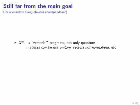
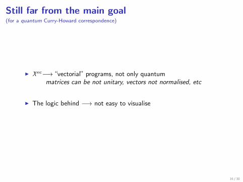
Still far from the main goal(for a quantum Curry-Howard correspondence)
I λvec−→ “vectorial” programs, not only quantummatrices can be not unitary, vectors not normalised, etc
I The logic behind −→ not easy to visualise
16 / 30
Still far from the main goal(for a quantum Curry-Howard correspondence)
I λvec−→ “vectorial” programs, not only quantummatrices can be not unitary, vectors not normalised, etc
I The logic behind −→ not easy to visualise
16 / 30
Outline
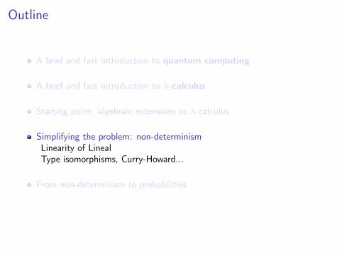
A brief and fast introduction to quantum computing
A brief and fast introduction to λ-calculus
Starting point: algebraic extensions to λ-calculus
Simplifying the problem: non-determinismLinearity of LinealType isomorphisms, Curry-Howard...
From non-determinism to probabilities
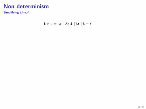
Non-determinismSimplifying Lineal
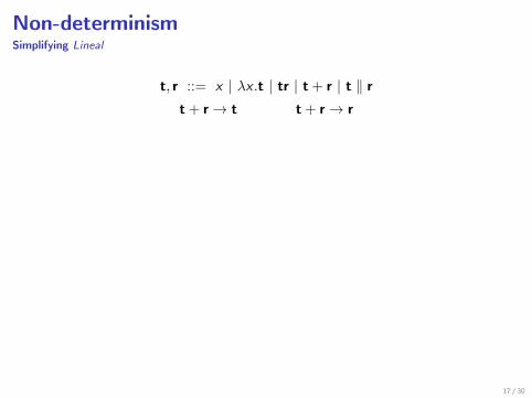
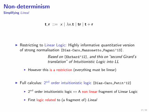
t, r ::= x | λx .t | tr | t + r
| t ‖ rt + r→ t t + r→ r
I Restricting to Linear Logic: Highly informative quantitative versionof strong normalisation [Díaz-Caro,Manzonetto,Pagani’13].
Based on [Ehrhard’12], and this on “second Girard’stranslation” of Intuitionistic Logic into LL
I However this is a restriction (everything must be linear)
I Full calculus: 2nd order intuitionistic logic [Díaz-Caro,Petit’12]
I 2nd order intuitionistic logic ↔ A non linear fragment of Linear Logic
I First logic related to (a fragment of) Lineal
17 / 30
Non-determinismSimplifying Lineal
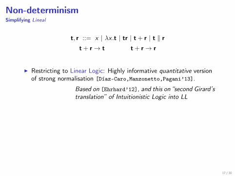
t, r ::= x | λx .t | tr | t + r | t ‖ rt + r→ t t + r→ r
I Restricting to Linear Logic: Highly informative quantitative versionof strong normalisation [Díaz-Caro,Manzonetto,Pagani’13].
Based on [Ehrhard’12], and this on “second Girard’stranslation” of Intuitionistic Logic into LL
I However this is a restriction (everything must be linear)
I Full calculus: 2nd order intuitionistic logic [Díaz-Caro,Petit’12]
I 2nd order intuitionistic logic ↔ A non linear fragment of Linear Logic
I First logic related to (a fragment of) Lineal
17 / 30
Non-determinismSimplifying Lineal
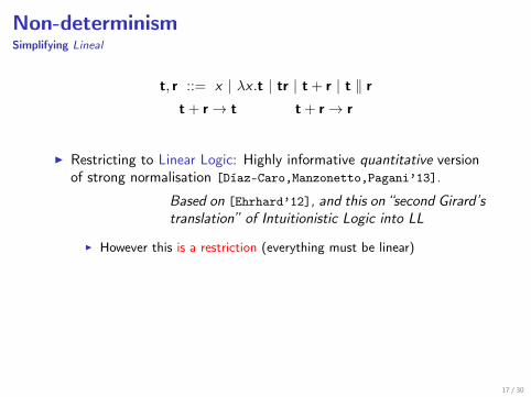
t, r ::= x | λx .t | tr | t + r | t ‖ rt + r→ t t + r→ r
I Restricting to Linear Logic: Highly informative quantitative versionof strong normalisation [Díaz-Caro,Manzonetto,Pagani’13].
Based on [Ehrhard’12], and this on “second Girard’stranslation” of Intuitionistic Logic into LL
I However this is a restriction (everything must be linear)
I Full calculus: 2nd order intuitionistic logic [Díaz-Caro,Petit’12]
I 2nd order intuitionistic logic ↔ A non linear fragment of Linear Logic
I First logic related to (a fragment of) Lineal
17 / 30
Non-determinismSimplifying Lineal
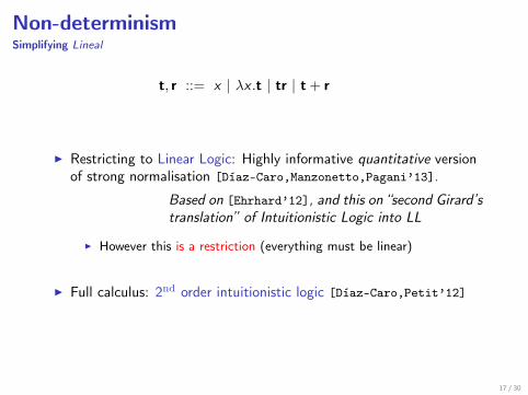
t, r ::= x | λx .t | tr | t + r
| t ‖ rt + r→ t t + r→ r
I Restricting to Linear Logic: Highly informative quantitative versionof strong normalisation [Díaz-Caro,Manzonetto,Pagani’13].
Based on [Ehrhard’12], and this on “second Girard’stranslation” of Intuitionistic Logic into LL
I However this is a restriction (everything must be linear)
I Full calculus: 2nd order intuitionistic logic [Díaz-Caro,Petit’12]
I 2nd order intuitionistic logic ↔ A non linear fragment of Linear Logic
I First logic related to (a fragment of) Lineal
17 / 30
Non-determinismSimplifying Lineal
t, r ::= x | λx .t | tr | t + r
| t ‖ rt + r→ t t + r→ r
I Restricting to Linear Logic: Highly informative quantitative versionof strong normalisation [Díaz-Caro,Manzonetto,Pagani’13].
Based on [Ehrhard’12], and this on “second Girard’stranslation” of Intuitionistic Logic into LL
I However this is a restriction (everything must be linear)
I Full calculus: 2nd order intuitionistic logic [Díaz-Caro,Petit’12]
I 2nd order intuitionistic logic ↔ A non linear fragment of Linear Logic
I First logic related to (a fragment of) Lineal
17 / 30
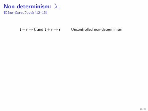
Non-determinism: λ+[Díaz-Caro,Dowek’12–13]
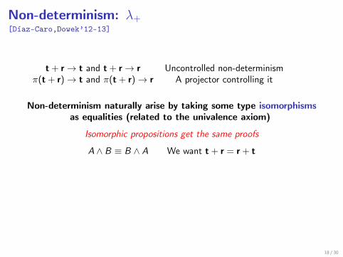
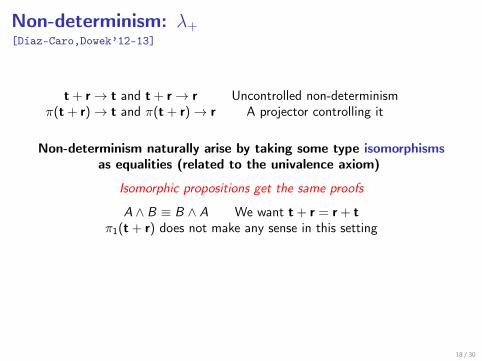
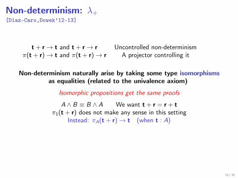
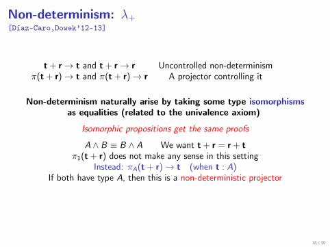
t + r→ t and t + r→ r Uncontrolled non-determinism
π(t + r)→ t and π(t + r)→ r A projector controlling it
Non-determinism naturally arise by taking some type isomorphismsas equalities (related to the univalence axiom)
Isomorphic propositions get the same proofs
A ∧ B ≡ B ∧ A We want t + r = r + tπ1(t + r) does not make any sense in this setting
Instead: πA(t + r)→ t (when t : A)If both have type A, then this is a non-deterministic projector
18 / 30
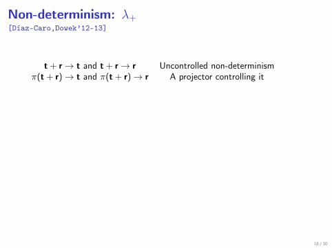
Non-determinism: λ+[Díaz-Caro,Dowek’12–13]
t + r→ t and t + r→ r Uncontrolled non-determinismπ(t + r)→ t and π(t + r)→ r A projector controlling it
Non-determinism naturally arise by taking some type isomorphismsas equalities (related to the univalence axiom)
Isomorphic propositions get the same proofs
A ∧ B ≡ B ∧ A We want t + r = r + tπ1(t + r) does not make any sense in this setting
Instead: πA(t + r)→ t (when t : A)If both have type A, then this is a non-deterministic projector
18 / 30
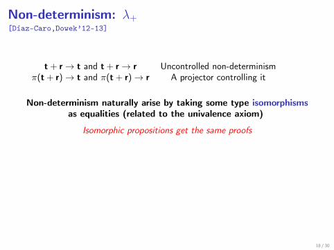
Non-determinism: λ+[Díaz-Caro,Dowek’12–13]
t + r→ t and t + r→ r Uncontrolled non-determinismπ(t + r)→ t and π(t + r)→ r A projector controlling it
Non-determinism naturally arise by taking some type isomorphismsas equalities (related to the univalence axiom)
Isomorphic propositions get the same proofs
A ∧ B ≡ B ∧ A We want t + r = r + tπ1(t + r) does not make any sense in this setting
Instead: πA(t + r)→ t (when t : A)If both have type A, then this is a non-deterministic projector
18 / 30
Non-determinism: λ+[Díaz-Caro,Dowek’12–13]
t + r→ t and t + r→ r Uncontrolled non-determinismπ(t + r)→ t and π(t + r)→ r A projector controlling it
Non-determinism naturally arise by taking some type isomorphismsas equalities (related to the univalence axiom)
Isomorphic propositions get the same proofs
A ∧ B ≡ B ∧ A We want t + r = r + t
π1(t + r) does not make any sense in this settingInstead: πA(t + r)→ t (when t : A)
If both have type A, then this is a non-deterministic projector
18 / 30
Non-determinism: λ+[Díaz-Caro,Dowek’12–13]
t + r→ t and t + r→ r Uncontrolled non-determinismπ(t + r)→ t and π(t + r)→ r A projector controlling it
Non-determinism naturally arise by taking some type isomorphismsas equalities (related to the univalence axiom)
Isomorphic propositions get the same proofs
A ∧ B ≡ B ∧ A We want t + r = r + tπ1(t + r) does not make any sense in this setting
Instead: πA(t + r)→ t (when t : A)If both have type A, then this is a non-deterministic projector
18 / 30
Non-determinism: λ+[Díaz-Caro,Dowek’12–13]
t + r→ t and t + r→ r Uncontrolled non-determinismπ(t + r)→ t and π(t + r)→ r A projector controlling it
Non-determinism naturally arise by taking some type isomorphismsas equalities (related to the univalence axiom)
Isomorphic propositions get the same proofs
A ∧ B ≡ B ∧ A We want t + r = r + tπ1(t + r) does not make any sense in this setting
Instead: πA(t + r)→ t (when t : A)
If both have type A, then this is a non-deterministic projector
18 / 30
Non-determinism: λ+[Díaz-Caro,Dowek’12–13]
t + r→ t and t + r→ r Uncontrolled non-determinismπ(t + r)→ t and π(t + r)→ r A projector controlling it
Non-determinism naturally arise by taking some type isomorphismsas equalities (related to the univalence axiom)
Isomorphic propositions get the same proofs
A ∧ B ≡ B ∧ A We want t + r = r + tπ1(t + r) does not make any sense in this setting
Instead: πA(t + r)→ t (when t : A)If both have type A, then this is a non-deterministic projector
18 / 30
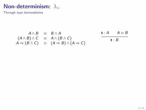
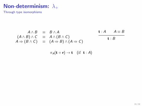
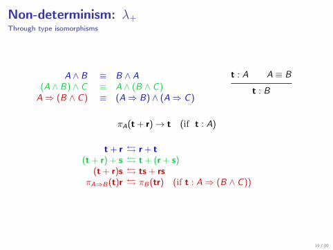
Non-determinism: λ+Through type isomorphisms
A ∧ B ≡ B ∧ A(A ∧ B) ∧ C ≡ A ∧ (B ∧ C )A⇒ (B ∧ C ) ≡ (A⇒ B) ∧ (A⇒ C )
t : A A ≡ B
t : B
πA(t + r)→ t (if t : A)
t + r r + t(t + r) + s t + (r + s)
(t + r)s ts + rsπA⇒B(t)r πB(tr) (if t : A⇒ (B ∧ C ))
19 / 30
Non-determinism: λ+Through type isomorphisms
A ∧ B ≡ B ∧ A(A ∧ B) ∧ C ≡ A ∧ (B ∧ C )A⇒ (B ∧ C ) ≡ (A⇒ B) ∧ (A⇒ C )
t : A A ≡ B
t : B
πA(t + r)→ t (if t : A)
t + r r + t(t + r) + s t + (r + s)
(t + r)s ts + rsπA⇒B(t)r πB(tr) (if t : A⇒ (B ∧ C ))
19 / 30
Non-determinism: λ+Through type isomorphisms
A ∧ B ≡ B ∧ A(A ∧ B) ∧ C ≡ A ∧ (B ∧ C )A⇒ (B ∧ C ) ≡ (A⇒ B) ∧ (A⇒ C )
t : A A ≡ B
t : B
πA(t + r)→ t (if t : A)
t + r r + t(t + r) + s t + (r + s)
(t + r)s ts + rsπA⇒B(t)r πB(tr) (if t : A⇒ (B ∧ C ))
19 / 30
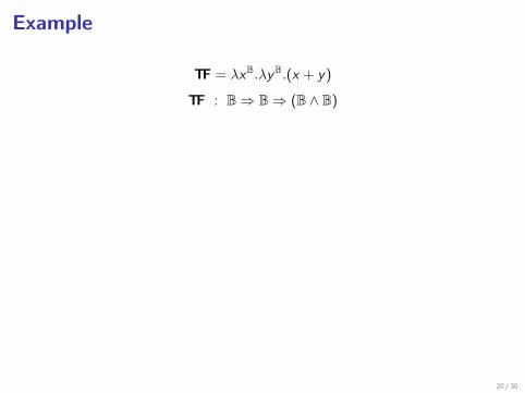
Example
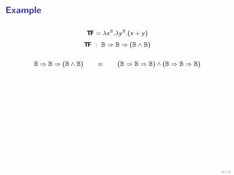
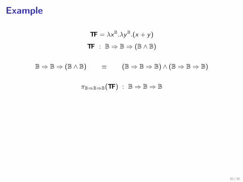
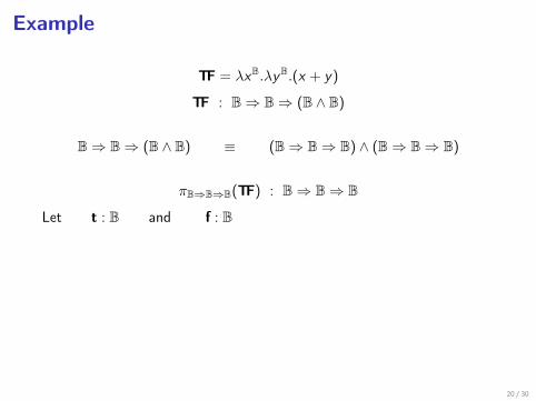
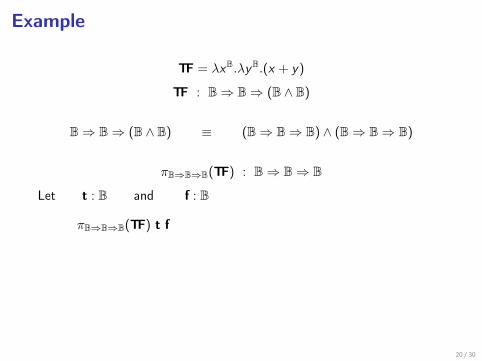
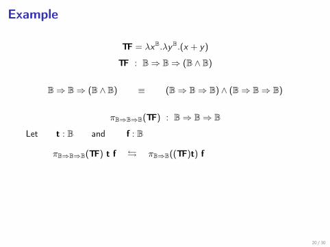
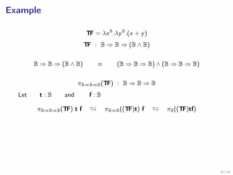
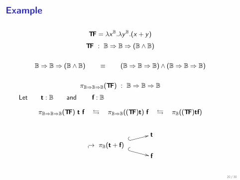
TF = λxB.λyB.(x + y)
TF : B⇒ B⇒ (B ∧ B)
B⇒ B⇒ (B ∧ B) ≡ (B⇒ B⇒ B) ∧ (B⇒ B⇒ B)
πB⇒B⇒B(TF) : B⇒ B⇒ B
Let t : B and f : B
πB⇒B⇒B(TF) t f πB⇒B((TF)t) f πB((TF)tf)
t
→ πB(t + f)%
33
y
++ f
20 / 30
Example
TF = λxB.λyB.(x + y)
TF : B⇒ B⇒ (B ∧ B)
B⇒ B⇒ (B ∧ B) ≡ (B⇒ B⇒ B) ∧ (B⇒ B⇒ B)
πB⇒B⇒B(TF) : B⇒ B⇒ B
Let t : B and f : B
πB⇒B⇒B(TF) t f πB⇒B((TF)t) f πB((TF)tf)
t
→ πB(t + f)%
33
y
++ f
20 / 30
Example
TF = λxB.λyB.(x + y)
TF : B⇒ B⇒ (B ∧ B)
B⇒ B⇒ (B ∧ B) ≡ (B⇒ B⇒ B) ∧ (B⇒ B⇒ B)
πB⇒B⇒B(TF) : B⇒ B⇒ B
Let t : B and f : B
πB⇒B⇒B(TF) t f πB⇒B((TF)t) f πB((TF)tf)
t
→ πB(t + f)%
33
y
++ f
20 / 30
Example
TF = λxB.λyB.(x + y)
TF : B⇒ B⇒ (B ∧ B)
B⇒ B⇒ (B ∧ B) ≡ (B⇒ B⇒ B) ∧ (B⇒ B⇒ B)
πB⇒B⇒B(TF) : B⇒ B⇒ B
Let t : B and f : B
πB⇒B⇒B(TF) t f πB⇒B((TF)t) f πB((TF)tf)
t
→ πB(t + f)%
33
y
++ f
20 / 30
Example
TF = λxB.λyB.(x + y)
TF : B⇒ B⇒ (B ∧ B)
B⇒ B⇒ (B ∧ B) ≡ (B⇒ B⇒ B) ∧ (B⇒ B⇒ B)
πB⇒B⇒B(TF) : B⇒ B⇒ B
Let t : B and f : B
πB⇒B⇒B(TF) t f
πB⇒B((TF)t) f πB((TF)tf)
t
→ πB(t + f)%
33
y
++ f
20 / 30
Example
TF = λxB.λyB.(x + y)
TF : B⇒ B⇒ (B ∧ B)
B⇒ B⇒ (B ∧ B) ≡ (B⇒ B⇒ B) ∧ (B⇒ B⇒ B)
πB⇒B⇒B(TF) : B⇒ B⇒ B
Let t : B and f : B
πB⇒B⇒B(TF) t f πB⇒B((TF)t) f
πB((TF)tf)
t
→ πB(t + f)%
33
y
++ f
20 / 30
Example
TF = λxB.λyB.(x + y)
TF : B⇒ B⇒ (B ∧ B)
B⇒ B⇒ (B ∧ B) ≡ (B⇒ B⇒ B) ∧ (B⇒ B⇒ B)
πB⇒B⇒B(TF) : B⇒ B⇒ B
Let t : B and f : B
πB⇒B⇒B(TF) t f πB⇒B((TF)t) f πB((TF)tf)
t
→ πB(t + f)%
33
y
++ f
20 / 30
Example
TF = λxB.λyB.(x + y)
TF : B⇒ B⇒ (B ∧ B)
B⇒ B⇒ (B ∧ B) ≡ (B⇒ B⇒ B) ∧ (B⇒ B⇒ B)
πB⇒B⇒B(TF) : B⇒ B⇒ B
Let t : B and f : B
πB⇒B⇒B(TF) t f πB⇒B((TF)t) f πB((TF)tf)
t
→ πB(t + f)%
33
y
++ f
20 / 30
Non-determinism: λ+
I A proof system where equivalent propositions get the same proofs
I Curry-Howard correspondence with 2nd order intuitionistic logic
I Non-deterministic projector
21 / 30
Outline
A brief and fast introduction to quantum computing
A brief and fast introduction to λ-calculus
Starting point: algebraic extensions to λ-calculus
Simplifying the problem: non-determinism
From non-determinism to probabilities
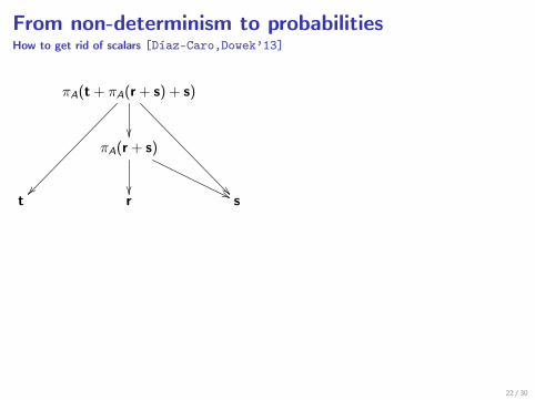
From non-determinism to probabilitiesHow to get rid of scalars [Díaz-Caro,Dowek’13]
πA(t + πA(r + s) + s)
πA(r + s)
''t r s
7→
πA(t + πA(r + s) + s)
13
13
13
πA(r + s)12
12
''t r s
∼ 13t +
16r +
12s
An easier way. . .
π(r + r + s + t + t + t)
r tt16
r zz16
s1
6
t 16
t$$16
t**16
22 / 30
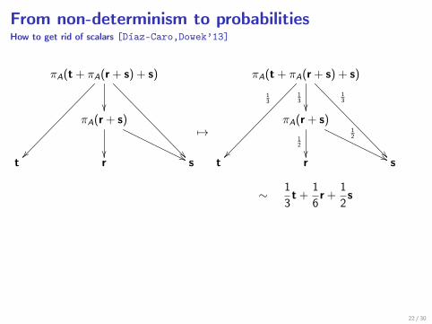
From non-determinism to probabilitiesHow to get rid of scalars [Díaz-Caro,Dowek’13]
πA(t + πA(r + s) + s)
πA(r + s)
''t r s
7→
πA(t + πA(r + s) + s)
13
13
13
πA(r + s)12
12
''t r s
∼ 13t +
16r +
12s
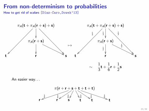
An easier way. . .
π(r + r + s + t + t + t)
r tt16
r zz16
s1
6
t 16
t$$16
t**16
22 / 30
From non-determinism to probabilitiesHow to get rid of scalars [Díaz-Caro,Dowek’13]
πA(t + πA(r + s) + s)
πA(r + s)
''t r s
7→
πA(t + πA(r + s) + s)
13
13
13
πA(r + s)12
12
''t r s
∼ 13t +
16r +
12s
An easier way. . .
π(r + r + s + t + t + t)
r tt16
r zz16
s1
6
t 16
t$$16
t**16
22 / 30
From non-determinism to probabilitiesGeneralising the problem to abstract rewrite systems
Idea: to define a variant of a Lebesgue measure for sets of realnumbers, on the space of traces
1st Define an intuitive measure on single rewrites
d
b
12 7712 // e
e.g. If a
13 <<
13 //13
""
cthen p(a→ c) = 1
3 + 13 and
p(a→ b;b→ d) = 13 ×
12 = 1
6
c
2nd Generalise it to arbitrary sets of rewrites taking the minimal cover withsets of single rewrites
Skip details
23 / 30
From non-determinism to probabilitiesGeneralising the problem to abstract rewrite systems
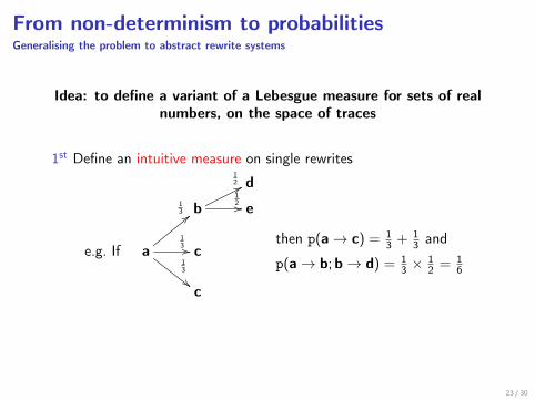
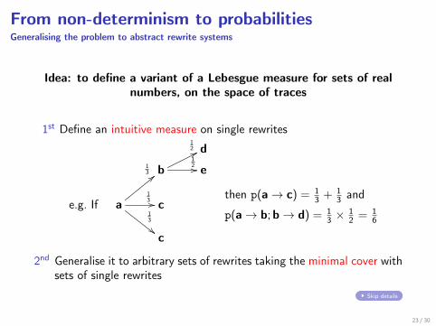
Idea: to define a variant of a Lebesgue measure for sets of realnumbers, on the space of traces
1st Define an intuitive measure on single rewrites
d
b
12 7712 // e
e.g. If a
13 <<
13 //13
""
cthen p(a→ c) = 1
3 + 13 and
p(a→ b;b→ d) = 13 ×
12 = 1
6
c
2nd Generalise it to arbitrary sets of rewrites taking the minimal cover withsets of single rewrites
Skip details
23 / 30
From non-determinism to probabilitiesStrategies
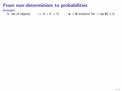
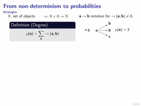
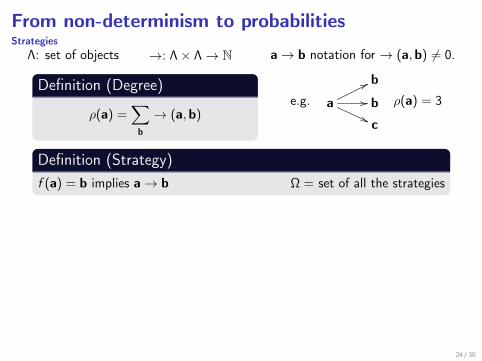
Λ: set of objects →: Λ× Λ→ N a→ b notation for → (a,b) 6= 0.
Definition (Degree)
ρ(a) =∑
b
→ (a,b)e.g.
b
a
77
//
''b
c
ρ(a) = 3
Definition (Strategy)f (a) = b implies a→ b Ω = set of all the strategies
e.g. Rewrite system
a
b c
d e
Ω = f , g , h, i, with
f (a) = b g(a) = bf (c) = d g(c) = e
h(a) = c i(a) = ch(c) = d i(c) = e
24 / 30
From non-determinism to probabilitiesStrategies
Λ: set of objects →: Λ× Λ→ N a→ b notation for → (a,b) 6= 0.
Definition (Degree)
ρ(a) =∑
b
→ (a,b)e.g.
b
a
77
//
''b
c
ρ(a) = 3
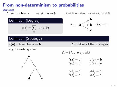
Definition (Strategy)f (a) = b implies a→ b Ω = set of all the strategies
e.g. Rewrite system
a
b c
d e
Ω = f , g , h, i, with
f (a) = b g(a) = bf (c) = d g(c) = e
h(a) = c i(a) = ch(c) = d i(c) = e
24 / 30
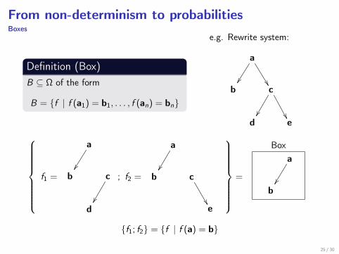
From non-determinism to probabilitiesBoxes
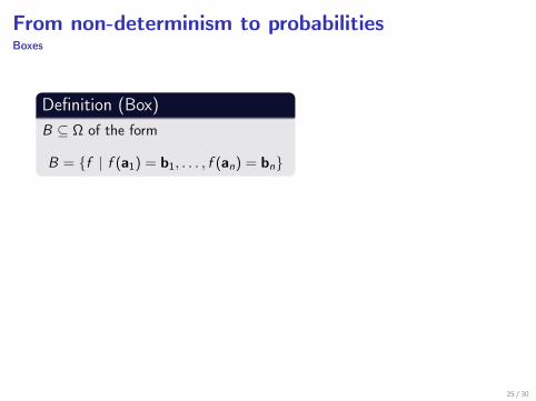
Definition (Box)B ⊆ Ω of the form
B = f | f (a1) = b1, . . . , f (an) = bn
e.g. Rewrite system:
a
b c
d e
f1 =
a
b c
d
; f2 =
a
b c
e
=
Boxa
b
f1; f2 = f | f (a) = b
25 / 30
From non-determinism to probabilitiesBoxes
Definition (Box)B ⊆ Ω of the form
B = f | f (a1) = b1, . . . , f (an) = bn
e.g. Rewrite system:
a
b c
d e
f1 =
a
b c
d
; f2 =
a
b c
e
=
Boxa
b
f1; f2 = f | f (a) = b
25 / 30
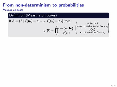
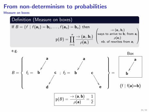
From non-determinism to probabilitiesMeasure on boxes
Definition (Measure on boxes)If B = f | f (a1) = b1, . . . , f (an) = bn then
p(B) =n∏
i=1
→ (ai ,bi )
ρ(ai )
→ (ai , bi )
ways to arrive to bi from aiρ(ai )
nb. of rewrites from ai
e.g.
B =
f1 =
a
b c
d
; f2 =
a
b c
e
=
Boxa
b
f | f(a)=b
p(B) =→ (a,b)
ρ(a)=
12
26 / 30
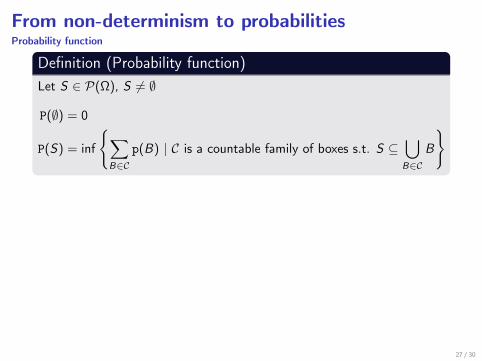
From non-determinism to probabilitiesProbability function
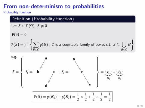
Definition (Probability function)Let S ∈ P(Ω), S 6= ∅
P(∅) = 0
P(S) = inf
∑B∈C
p(B) | C is a countable family of boxes s.t. S ⊆⋃B∈C
B
e.g.
S =
f1 =
a
b c
d
; f2 =
a
c
e
= f1︸︷︷︸
B1
∪ f2︸︷︷︸B2
P(S) = p(B1) + p(B2) =12× 1
2+
12× 1
2=
12
27 / 30
From non-determinism to probabilitiesProbability function
Definition (Probability function)Let S ∈ P(Ω), S 6= ∅
P(∅) = 0
P(S) = inf
∑B∈C
p(B) | C is a countable family of boxes s.t. S ⊆⋃B∈C
B
e.g.
S =
f1 =
a
b c
d
; f2 =
a
c
e
= f1︸︷︷︸
B1
∪ f2︸︷︷︸B2
P(S) = p(B1) + p(B2) =12× 1
2+
12× 1
2=
12
27 / 30
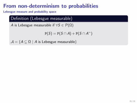
From non-determinism to probabilitiesLebesgue measure and probability space
Definition (Lebesgue measurable)A is Lebesgue measurable if ∀S ∈ P(Ω)
P(S) = P(S ∩ A) + P(S ∩ A∼)
A = A ⊆ Ω | A is Lebesgue measurable
Theorem(Ω,A, P) is a probability space
I Ω is the set of all possible strategiesI A is the set of eventsI P is the probability function
Proof.We show that it satisfies the Kolmogorov axioms.
28 / 30
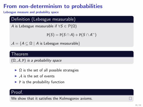
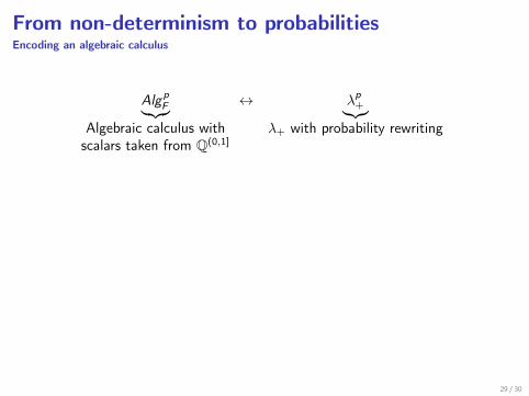
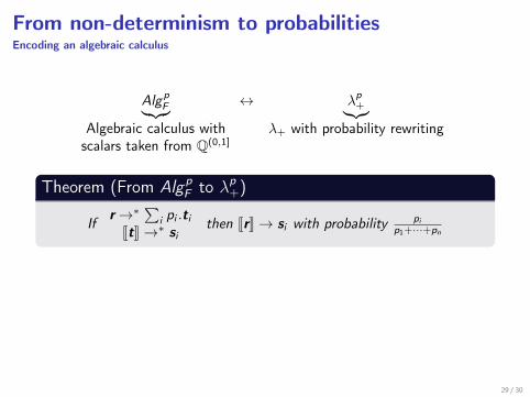
From non-determinism to probabilitiesEncoding an algebraic calculus
AlgpF︸︷︷︸
Algebraic calculus withscalars taken from Q(0,1]
↔ λp+︸︷︷︸
λ+ with probability rewriting
Theorem (From AlgpF to λp
+)
If r→∗∑
i pi .tiJtK→∗ si
then JrK→ si with probability pip1+···+pn
Theorem (From λp+ to Algp
F )r→∗ ti with probability pi , for i = 1, . . . , n ⇒ LrM→∗
∑i pi .Lti M
29 / 30
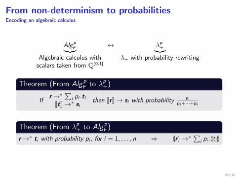
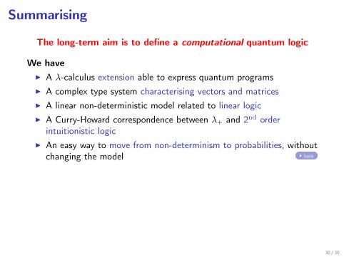
Summarising
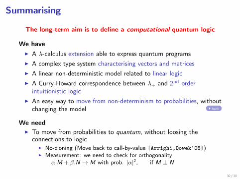
The long-term aim is to define a computational quantum logic
We haveI A λ-calculus extension able to express quantum programsI A complex type system characterising vectors and matricesI A linear non-deterministic model related to linear logicI A Curry-Howard correspondence between λ+ and 2nd order
intuitionistic logicI An easy way to move from non-determinism to probabilities, without
changing the model back
We needI To move from probabilities to quantum, without loosing the
connections to logicI No-cloning (Move back to call-by-value [Arrighi,Dowek’08])I Measurement: we need to check for orthogonality
α.M + β.N → M with prob. |α|2, if M ⊥ N
30 / 30
Summarising
The long-term aim is to define a computational quantum logic
We haveI A λ-calculus extension able to express quantum programsI A complex type system characterising vectors and matricesI A linear non-deterministic model related to linear logicI A Curry-Howard correspondence between λ+ and 2nd order
intuitionistic logicI An easy way to move from non-determinism to probabilities, without
changing the model back
We needI To move from probabilities to quantum, without loosing the
connections to logicI No-cloning (Move back to call-by-value [Arrighi,Dowek’08])I Measurement: we need to check for orthogonality
α.M + β.N → M with prob. |α|2, if M ⊥ N
30 / 30